What is computational fluid dynamics?

Computational fluid dynamics is a technique that determines the behaviour of fluid flow using the laws of physics. In haemodynamics, these laws are the law of conservation of mass, conservation of linear momentum, embodied in Newton's laws of motion, and the laws of thermodynamics. The relevant physical properties of the materials under consideration – for example, density and viscosity – must also be known. In spite of this apparent complexity, the calculation of blood flow in biological systems is relatively straightforward, avoiding many of the features of more complicated fluid flow phenomena. The laws in differential form are expressed by the Navier–Stokes equations, as follows:

$$\nabla \cdot \vec {V}\, = \,0 \ and \ \rho \frac{{\partial \vec {V}}}{{\partial t}}\, + \,\rho (\vec {V} \cdot \nabla )\vec {V}\, = \,{\rm{ - }}\nabla p\, + \,\nabla \cdot \tau $$

where ρ denotes the fluid density, μ denotes the fluid viscosity, τ denotes the viscous stress tensor, p is the pressure, and $$)(--><$>\vec {V}<$><!--$$ denotes the velocity vector. Although these equations are non-linear and generally cannot be solved analytically, they can always be solved using numerical techniques. Such techniques, most commonly finite volume or finite element methods, form the basis of computational fluid dynamics and use the fact that all differentials or integrals can be computed by approximating infinitesimally small changes (dx) as small but finite changes (Δx). A differential, or an integral, however complicated, is reduced to an analogous algebraic expression. Utilising this principle along with an appropriate accompanying representation of the continuum of interest by a distributed set of mesh points, or finite elements, produced by the process of mesh generation, an algebraic – discrete – analogue to the continuous problem is obtained over each gird volume or finite element, see Figure 1.Reference Ceballos, Argueta-Morales and Divo ¹ The resulting set of non-linear algebraic equations, which can number in the millions of equations, can be solved iteratively using computer workstations or clusters of workstations. Typically, resolving a time-accurate solution can take upwards of 2 or more days of computations.

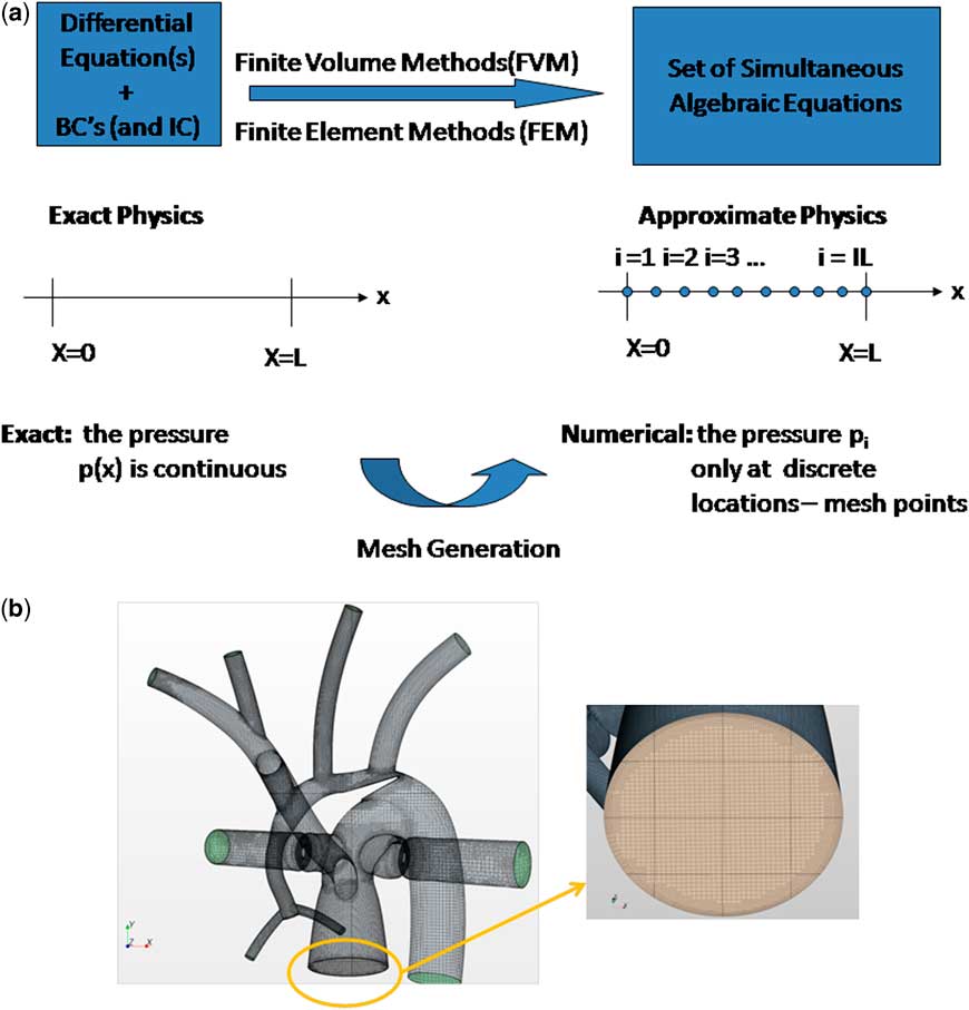
Figure 1 (a) Numerical methods generate an algebraic analogue to the continuous problem, (b) Example of a finite volume method mesh used for an analysis of the hybrid Norwood operation.Reference Ceballos, Argueta-Morales and Divo ¹ Here nearly 1.2 million cells are used to discretise the three-dimensional volume of interest for the haemodynamics analysis. (left) Hybrid Norwood topology with distal arch obstruction, (right) close-up of pulmonary root mesh. BC = boundary conditions; FEM = finite element methods; FVM = finite volume methods; IC = initial conditions.

Solving the equations of fluid flow requires that certain initial conditions and fixed conditions must be specified a priori. Examples include the resistances of vascular beds, parameters of the cardiac elastance function, and geometry – vessel size, shape, branching pattern, etc. – of the region of interest. In addition, a priori boundary conditions must be satisfied. Boundary conditions are imposed values of the calculated quantities – for example, velocity and pressure – at certain locations and times. For example, the velocity of flow at the inner surface of a blood vessel must be zero. Boundary conditions may be imposed by use of experimental or clinical information, such as catheter or magnetic resonance imaging data. In general, magnetic resonance data provide excellent velocity and flow, but not pressure data. Invasive catheterisation can provide some pressure information but at poor special resolution. In this sense, computational fluid dynamics is not always a purely theoretical but may be a semi-empirical method that can calculate accurate pressure information at high resolution. Boundary conditions are satisfied by adjusting the solution in an iterative manner until the conditions are met. Sometimes, the boundary conditions themselves must be calculated from systems, often on a different scale, to which they are coupled. For example, we may be interested in the detailed flow characteristics in the aortic arch, using computational fluid dynamics. The “inlet” and “outlet” boundary conditions will be the flows and pressures at the aortic root, arch great vessels, and the distal arch (Fig 2).

Figure 2 Inlet (aortic root) and outlet (great vessels) boundary conditions for the aortic arch. AO = aorta; DA = descending aorta; IA = innominate artery; LCA = left carotid artery; LSA = left subclavian arteries; RCA = right carotid artery; RSA = right subclavian artery.

These boundary flows and pressures, however, depend on cardiac function, and on the characteristics of all peripheral arterial beds, and hence must also be solved for. We refer to such problems as “multi-scale” problems. Computational fluid dynamics may not be required to compute the solution at the other scale, as parameterised – “lumped parameter” – models may suffice and save considerable computational time without loss of accuracy and physical meaning. A representative multi-scale design for analysing the Norwood circulation is shown in Figure 3.Reference Ceballos, Argueta-Morales and Divo ¹ In general, the extent to which a multi-scale solution is required depends on what one is attempting to demonstrate in the “region of interest”.

Figure 3 Multi-scale design for analysing the hybrid Norwood circulation.

Computational fluid dynamics is not a technique of simulation – it is a technique of calculation. In simulation, the behaviour of the phenomenon is generally already known. The objective of simulation is to reproduce the behaviour as realistically as possible, for application to training or to product testing. In computational fluid dynamics, the answer is not known ahead of time, and the method hence discovers the behaviour of fluid phenomena. The accuracy of the calculation is as good as that of the input initial and boundary conditions, and the precision is as good as the “fineness” of the finite volumes, or finite elements, and the theoretical power of the numerical technique used. The current capability of parallel processing allows very precise solution to the three-dimensional Navier–Stokes equations in non-steady haemodynamic flows within reasonable computational time. Typically not included in computational fluid dynamics calculations are biological effects such as auto-regulation, healing, and growth. Moreover, in most reported analysis the detailed compliance of the vessel walls is not taken into account, although there is a trend to include such a phenomenon through fluid-structure interaction modelling,Reference Long, Hsu, Bazilevs, Feinstein and Marsden ^{2 ,} Reference Humphrey and Holzapfel ³ although models are still limited by the availability of constitutive models for the arterial wall.Reference Gasser, Ogden and Holzapfel ⁴

What can computational fluid dynamics tell us?

One's ability to intuit fluid flow is limited by the non-linear nature of the behaviour itself while computational fluid dynamics is able to provide such detailed solutions of the behaviour of fluid flow. From the computational solution, a myriad of phenomena can be described (Table 1). Many of these phenomena have been linked empirically to pathological changes in cardiovascular structure and function. Thus, not only may computational fluid dynamics lead to the pathophysiology and mechanism of disease, but it may also lead to preventative or therapeutic measures to circumvent the disease.

Table 1 Examples of flow phenomena that can be characterised by CFD.

CFD = computational fluid dynamics

Superior and total cavopulmonary connections

Some of the earliest work using computational fluid dynamics in congenital heart disease was applied to solving the optimal anatomic configuration of the superior cavopulmonary connection. As the pulmonary flow in such physiology is passive, it was believed that minimisation of flow energy loss, as well as the equal balance of flows to the left and right lungs, was at least theoretically related to clinical functional capacity and perhaps longevity. In these analyses, the usual endpoints of the calculation were (1) the ratio of left pulmonary artery and right pulmonary artery flow rate and (2) the fraction of incoming hydraulic power dissipated, with the hydraulic power being defined as

$$W\, = \,\big(\frac{1}{2}\rho {{V}^{\rm{2}}} \, + \,p\big)Q$$

where ρ is the density of blood and V, p, and Q are the mean velocity, pressure, and flow rate, respectively, at each inlet and outlet of the region of interest – specifically, the caval vein, hepatic veins, and branch pulmonary arteries at the lung hila. The fractional power dissipated was defined as ( W_{inle t} − W_outlet )/ W_inlet . This value is in the range of 1 mW in a typical Fontan configuration. The optimal surgical configuration was defined as that which rendered the minimum fractional power dissipation and the best balance of left and right lung flows. In the earliest work,Reference de Leval, Dubini and Migliavacca ⁵ it was predicted that the optimal configuration was that of the inferior cavopulmonary connection “extended” towards the right pulmonary artery relative to the superior caval connection. These early predictions were limited by a priori knowledge of input boundary conditions – from limited magnetic resonance velocity data – as well as the lack of consideration of vessel elasticity and the effects of ventilation. Over the next 15 years, considerable improvements were made in these calculations owing to (1) better resolution of magnetic resonance imaging, (2) improved computing power, and (3) the use of real patient data to configure the anatomy. Hsia et alReference Hsia, Migliavacca and Pittaccio ⁶ recalculated the cavopulmonary optimisation scheme, comparing the lateral tunnel, intra-atrial tube, and extracardiac conduit – offset to the left or to the right of the superior caval anastomosis. They found the optimal configuration to be that of a 19–20-mm extracardiac conduit offset to the left of the superior caval vein. Much smaller, and much larger diameter conduits had greater power loss. The range in fractional power loss was not very large: 0.081 for the optimal configuration and 0.11 for the conduit offset to the right of the superior caval vein, and the range in left to right lung flow ratio was 0.9 to 1.1. Socci et alReference Socci, Gervaso and Migliavacca ⁷ and Sundareswaran et alReference Sundareswaran, Pekkan and Dasi ⁸ confirmed many of the flow characteristics in further analyses.

Marsden et alReference Marsden, Bernstein and Reddy ⁹ investigated the fluid dynamics of a Y-graft configuration for the inferior cavopulmonary connection in a patient-specific model using magnetic resonance data and computational fluid dynamics. Their study included a model for ventilator effect and for exercise, the latter being modelled simply as an increase in input flow rate. Compared with standard single extracardiac conduits – with and without offset – the Y-graft with 12-mm-diameter branches had (1) lower fractional power dissipation during rest and exercise, (2) lower superior caval vein pressure during exercise, (3) greater equilibration of left and right lung flow, and (4) larger regions of low shear stress.

Whitehead et alReference Whitehead, Pekkan, Kitajima, Paridon, Yoganathan and Fogel ¹⁰ further investigated power dissipation during modelled exercise. They used resting magnetic resonance data from 10 patients and thus generated 10 baseline models to investigate. They determined the presence of a non-linear relation between flow rate – the exercise parameter – and power dissipation. An exercise level of three times baseline flow resulted in power dissipation equivalent to nearly doubling the pulmonary vascular resistance. They argued that this effect could substantially increase “Fontan pressures”, as well as limit effective cardiac output. They also found that pulmonary flow splits substantially affected power dissipation.

Itatani et alReference Itatani, Miyaji and Tomoyasu ¹¹ investigated the effect of conduit diameter on power dissipation and on the volume of flow stagnation, that is, regions of flow velocity <1 cm/s. They used velocity and flow data from 17 Fontan patients to form input boundary conditions and to design the representative anatomy. These data included clinical magnetic resonance velocities both a rest and two levels of exercise. They also modelled ventilation. Using computational fluid dynamics, they found resting power dissipation of 1.5–1.7 mW, or 6–7% of input power. At 1 W/kg exercise, power dissipation was 4–6 mW, or 9.6–12.5% of input power. The dependence on conduit sizes, ranging from 14 to 22 mm, was monotonic and most pronounced during 1 W/kg exercise – the larger the conduit, the less the power dissipation. Larger conduits, however, were associated with greater stagnation volume. The greatest stagnation volumes occurred at rest, in the expiratory ventilator phase, and in the larger – 20–22 mm– conduits. The value reached 5.2 ml, or 34% of the 22-mm conduit volume. The authors suggested the optimal conduit size to be in the 18–19-mm range.

Norwood procedure and variants

Computational fluid dynamics studies of the Norwood circulation began with an analysis, by Migliavacca et al,Reference Migliavacca, Dubini and Pennati ¹² of flow in a systemic to pulmonary artery shunt. They investigated the shunt pressure drop–flow relationship, varying shunt implantation angle, diameter, curvature, and input pulsatility and found, as expected, that shunt diameter was the main determinant of graft flow. Most of the pressure drop occurred near the proximal anastomosis, and curved grafts resulted in a lower pressure drop as compared with straight grafts, owing to reduced flow-line skewness towards the lateral graft wall near the proximal anastomosis. They found that inertial effects – pulsatility – had little influence on the solutions. In a follow-up study,Reference Migliavacca, Pennati and Dubini ¹³ they investigated the Norwood circulation using a three-compartment “lumped-parameter” model, using available clinical data to derive input and boundary conditions. The compartments included the heart model, and systemic and pulmonary circulations. They varied shunt sizes from 3–5 mm and determined that larger shunt diameters diverted cardiac output to the lungs, thereby diminishing O₂ delivery and that maintaining a pulmonary to systemic blood flow ratio of 1 provided optimal O₂ delivery across investigated heart rate and shunt size combinations. From the computational fluid dynamics solutions, they derived expressions that allowed clinical estimation of shunt flow from Doppler-derived pressure drop data.Reference Migliavacca, Yates, Pennati, Dubini, Fumero and de Leval ¹⁴

Multi-scale computational fluid dynamics analysis of the variants of the Norwood reconstructive surgeries were compared with post-operative catheterisation and Doppler data.Reference Migliavacca, Balossino and Pennati ^{15 ,} Reference Bove, Migliavacca and de Leval ¹⁶ In these studies, the Norwood operation with a modified Blalock–Taussig shunt was compared with the right ventricle-to-pulmonary artery shunt modification. They found good correlation between computational fluid dynamics solutions and observed post-operative clinical data, further buttressing confidence in the predictive capabilities of the multi-scale computational fluid dynamics analysis as an effective tool for pre-operative planning. The model predicted that the right ventricle shunt would result in higher aortic diastolic pressure, decreased pulmonary arterial pressure, lower pulmonary to systemic flow, and higher coronary perfusion relative to the innominate artery-to-right pulmonary artery shunt. Moreover, examination of detailed flow profiles in the right ventricle-to-pulmonary artery shunt led the authors to predict minimal regurgitation through the conduit, which was consistent with clinical measurements. The size of the shunt is critical for the innominate artery-to-right pulmonary artery operation as the larger shunts lead to detrimental haemodynamics, although larger shunts are needed for the right ventricle shunt to achieve satisfactory arterial oxygenation. The authors report a non-intuitive result predicted by the model, namely, that the afterload in the right ventricle-to-pulmonary artery configuration is lower than that of the innominate artery-to-right pulmonary artery configuration because of flow through the right ventricle shunt before the aortic valve opening, resulting in reduced ventricular wall shear stress at equal pressure. In a follow-up study, Hsia et alReference Hsia, Migliavacca and Pennati ¹⁷ utilised multi-scale analysis in a surgical planning setting to compare alternatives to management of stenotic right ventricle-to-pulmonary artery shunt after the Norwood procedure, namely: (1) conversion to a modified Blalock–Taussig shunt and (2) augmenting the existing right ventricle-to-pulmonary artery shunt with an additional modified Blalock–Taussig shunt. They concluded that the second option can lead to pulmonary overcirculation and recommended that the stenotic shunt be taken down and conversion to an optimal modified Blalock–Taussig shunt be undertaken.

Multi-scale computational fluid dynamics analysis has been applied to study another variant, the so-called hybrid Norwood approach. A multi-scale computational fluid dynamics analysis was used by Corsini et alReference Corsini, Cosentino, Pennati, Dubini, Hsia and Migliavacca ¹⁸ to examine the role of the stented arterial duct and the degree of pulmonary banding to achieve the balance of Q_p/Q_s , cardiac output, and O₂ delivery to optimize patient survival in the hybrid Norwood. They concluded that oxygen delivery was most sensitive to the degree of branch pulmonary banding rather than to the ductal stent size. Ceballos et alReference Ceballos, Argueta-Morales and Divo ^{1 ,} Reference Ceballos, Kassab and Osorio ¹⁹ utilised a multi-scale analysis of the hybrid Norwood operation using a synthetic but anatomically appropriate reconstruction of the vasculature and considered the effect of distal arch obstruction on the hybrid Norwood circulation with and without the presence of a reverse Blalock–Taussig shunt from the pulmonary root to the innominate artery.

The analysis showed that a 90% distal arch stenosis reduced pressure and net flow rate through the coronary and carotid arteries by 30% (Table 2 and Fig 4). Addition of a 4-mm × 21-mm reverse Blalock–Taussig shunt completely restored pressure and flow rate to baseline in these vessels. Zones of flow stagnation, flow reversal, and recirculation in the presence of stenosis were rendered more orderly by addition of the reverse Blalock–Taussig shunt. In the absence of stenosis, a “preventatively” placed shunt resulted in extensive zones of disturbed flow within the reverse Blalock–Taussig shunt consisting of zones with thrombogenic potential (recirculation and stagnation that persist for a substantial fraction of the cardiac cycle) (Fig 5; see Supplementary Material, Videos 1 and 2).

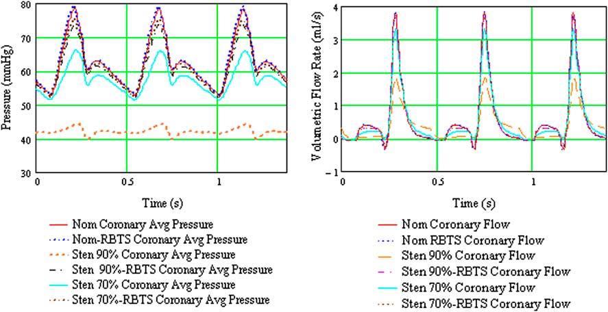
Figure 4 Composite plot of average coronary pressure and flow for the six configurations considered for the hybrid Norwood analysis. mmHg = millimetres of mercury; Nom = nominal (baseline model, no aortic arch stenosis); RBTS = reverse Blalock–Taussig shunt; s = seconds; Sten 90 = model with 90% distal aortic arch obstruction; Sten 70% = model with 70% distal arch obstruction.

Table 2 Results from multi-scale CFD analysis of six configurations considered in the hybrid Norwood operation – Cardiac output, arterial flow rates, and flow changes for all anatomical configurations.

DA = descending aorta; LCA = left carotid artery; LcorA = left coronary artery; LPA = left pulmonary artery; LSA = left subclavian artery; Qp/Qs = pulmonary to systemic flow ratio; RBTS = reverse Blalock–Taussig shunt; RCA = right carotid artery; RcorA = right coronary artery; RPA = right pulmonary artery; RSA = right subclavian artery

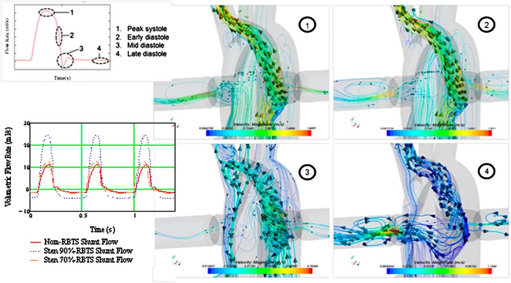
Figure 5 Close-up examination of the reverse Blalock–Taussig shunt graft flow when the shunt is placed “preventatively”, that is, before significant distal arch obstruction develops. Detailed pathlines exhibit swirling flow with several zones of recirculation and low velocity for a good fraction of the cardiac cycle. Nom = nominal (baseline model, no aortic arch stenosis); RBTS = reverse Blalock-Taussig shunt; Sten 90% = model with 90% distal aortic arch obstruction; Sten 70% = model with 70% distal arch obstruction.

Optimisation of left ventricular assist device implantation to reduce stroke risk

Using computational fluid dynamics studies, Osorio et alReference Osorio, Osorio and Ceballos ²⁰ and Argueta-Morales et alReference Argueta-Morales, Tran, Clark, Divo, Kassab and DeCampli ²¹ reported as much as a 50% reduction of cerebral thromboembolism by tailoring of the angle and placement of the of ventricular assist device outflow cannula in adult computer-generated and patient-specific calculations. The flow field was resolved in the steady state, representative of low pulsatility conditions of continuous-flow assist devices, and thrombus paths were computed using a Lagrangian model. The trajectories of smaller size particles – (thrombi) with low momentum essentially followed the streamlines, whereas those of larger particles with higher momentum deviated from the streamlines (see Supplementary Material, Videos 3 and 4). Computations to study blood flow patterns and particle tracks originating in the assist device were carried out on representative three-dimensional aortic arch models for Infant (4 kg) and Child (20 kg) models.Reference DesJardins, Argueta-Morales and Ceballos ²² The percentage of particles entering cerebral vessels was calculated for 14 implantation configurations for an 8-mm assist device outflow graft. Figure 6 shows flow pathlines for three different implantation angles. For both models, the percentage of particles entering the cerebral vessels varied by as much as 50% depending on the implantation configuration. In the Infant model, there is a “smoother” transition of flow into the aortic arch because the assist device outflow graft diameter is equal to the ascending aorta. Decreasing the anastomosis angle directs the blood flow straight into the cerebral vessels, resulting in an increased risk of embolisation. In the Child model, shallower angle and more cephalad placement of the assist device outflow graft anastomosis prevents formation of recirculation zones in the ascending aorta, decreasing the cerebral embolisation rate (see Supplementary Material, Videos 5 and 6).

Figure 6 The Infant model flow pathlines for perpendicular (left), intermediate (middle), and shallow (right) ventricular assist device outflow graft anastomotic angles. These three models resulted in significantly different probabilities of cerebral thromboembolism from thrombi originating proximal to the distal end of the assist device outflow graft.