Definition of a Chronic Condition

The chronic conditions health states that we define must be interpretable as irreversible. Not all chronic conditions covered by surveys satisfy that requirement, and whether they do may depend on the wording of the questions. Consider, for example, the following alternative wordings of a question about cancer: (1) “Do you have cancer?” (2) “Have you ever been diagnosed with cancer?” A survey respondent who had a cancerous tumour successfully removed surgically could have said “yes” to question (1) just before the surgery but “no” to the same question five years later if all follow-up tests had been negative. However, the same respondent would have had to say “yes” to question (2) at both times. Thus, by inference, the condition is reversible in the first case, irreversible in the second. Cataracts (removable by surgical lens implantation) provide a second example in which the wording of the question is important; hypertension (treatable by dietary change or drug therapy) provides a third. In addition to flows among health states, we are concerned with deaths – flows into the “dead state”, which is obviously an irreversible or “absorbing” state.

The importance of irreversibility for our purposes is that it means that net flows of population from one state to another can be interpreted as gross flows. That is the key idea that allows us to construct state transition matrices from chronic conditions survey data.

Similarity and Consistency with the Life Table

The similarity of our framework with the approach taken in constructing a life table comes about as follows. The standard life table is derived from age-specific death probabilities based on the observed population mortality rates of a given year. It draws out the implications of the death probabilities for survival and life expectancy at different ages. The survivors then constitute a stationary population, one in which the population size and age distribution remain constant over time. The life table represents a useful tool for studying the implications of the probabilities current at a given time. What we do, as this article explains, is similar in that we calculated age-specific probabilities of transition among health and mortality states based on data at a given time and derive the implications of those probabilities for a stationary population in which they remain unchanged. One can experiment with changes in the life table death probabilities and calculate the resultant new stationary population (see Keyfitz & Carswell, Reference Keyfitz and Carswell2005, chapter 14, for example); in the same way, one can (as we do) experiment with changes in health state transition probabilities and observe the consequences.

The consistency of our framework with the standard life table arises from the fact that life table death probabilities are incorporated directly into the framework. The overall probability of dying between some age x and subsequent age x + 1 serves as a control on the health-state-specific probabilities of dying; the overall probability at each age is, in effect, allocated among health state components. The transition probabilities thus relate to a stationary population identical, in demographic characteristics, to the life table population.

Transition Flows and Probabilities

In this section we present a formal description of the transition model. Let x stand for age and assume a population of given size at some initial age (call it x = 0). Assume also n (irreversible) chronic conditions. At any age x > 0, a member of the initial population may have contracted none of these conditions, one of them, two of them, three of them, and so on, or may be dead. The total number of health states at any age (including good health and the dead state) is then G(n) = $\sum\limits_{r = 0}^n {nCr + 1}$ where nCr is the “n select r” combinatorics symbol.

Now visualize a transition flow matrix F for some age x. The rows represent the possible health states at age x, and the columns represent the same states at x + 1; a typical element, f _ij , represents the number of people who move from state i to state j. With n individual chronic conditions, F is a G(n) × G(n) matrix with G(n)^{Footnote 2} elements. If n = 3, for example, F is 9 × 9 and there are 81 elements. If n = 4, F is 17 × 17; if n = 5, F is 33 × 33. Thus, the size of the matrix rises rapidly as n increases. However, not all elements represent admissible flows; many are zero because of the irreversibility.

Anticipating our numerical application, we identify three chronic conditions, and thus a 9 × 9 flow matrix. The conditions are cancer, C; stroke/heart condition, S; and diabetes, D. All other conditions are collapsed into what we call the “healthy” state, defined as alive, with an absence of C, S, and D, and denoted by H; the dead state is denoted by X. The nine states are then H, C, S, D, CS, CD, SD, CSD, and X, where a double-letter state indicates the presence of two chronic conditions; the triple-letter state, the presence of all three. Someone in H can move to any of the other states. Someone in C, say, can remain in the same state or move only to CS, CD, CSD, or X; someone in CS can move only to CSD or X. That is, once a “C label” is attached to an individual, only X or a state that also has a C label is attainable.

The form of the 9 × 9 flow matrix is shown in Table 1. A check mark indicates that a flow is admissible; a 0, that it is not. Of the 81 elements in the matrix, 36 are admissible, 45 are inadmissible. In general, for a G(n) × G(n) matrix, K(n) = G(n)^{Footnote 2} is the total number of elements in F. The number of positive (that is, admissible) elements is then given by

K(n,+) = G(n) + $\sum\limits_{q = 1}^{n - 1} {nCq[2 + } \sum\limits_{k = 1}^n {(n - q)Ck]}$ + 3.

Table 1: Admissible (√) and inadmissible (0) elements of the flow matrix

The transition probability matrix, P, is derived from F in a straightforward manner. Let F_i. be the (positive) row i total and let p _ij, the i,j element of P, be the probability of moving from state i at age x to state j at age x + 1. Given the flow matrix F, the calculation is then p_ij = f_ij/F_i. (i,j = 1,2, … ,G(n)).

Interpreting the Death Probabilities

The probability of dying for someone in the C state is not the probability of dying from cancer. Rather, it is the probability of dying for any reason for someone who has been diagnosed with cancer. Someone who has been so diagnosed may indeed die of cancer but he/she may also die as a result of some other cause.

There is a large and informative literature analysing the probabilities of dying, by cause of death, and the effects of reducing or eliminating particular causes. (The elimination of cancer has received considerable attention, for example.) Without attempting to be exhaustive, we note the following: an early contribution is Keyfitz (Reference Keyfitz1977); a selection of more recent ones includes Nusselder, van der Velden, van Sonsbeek, Lenior, and van den Bos (Reference Nusselder, van der Velden, van Sonsbeek, Lenior and van den Bos1996); Mackenbach, Kunst, Lautenbach, Oei, and Bijlsma (Reference Mackenbach, Kunst, Lautenbach, Oei and Bijlsma1999); Manuel, Luo, Ugnat, and Mao (Reference Manuel, Luo, Ugnat and Mao2003); Kintner (Reference Kintner, Siegel and Swanson2004; see “Cause-Elimination Life Tables”); Somerville and Francombe (Reference Somerville and Francombe2005); and Beltrán-Sánchez, Preston, and Canudas-Romo (Reference Beltrán-Sánchez, Preston and Canudas-Romo2008). This literature makes use of cause-of-death data originating with registered death certificates. Our present study has some obvious kinship with it, but our framework, data source, definitions, and intended application differ. We construct a comprehensive system that encompasses transitions among health states as well as the associated mortality probabilities. We draw our data from surveys of chronic conditions rather than death registrations. Finally, and importantly, our death probabilities for people with given chronic conditions are the probabilities of dying from any cause, not just from those conditions.

An Age Sequence of Transition Matrices

Assume a sequence of ages or age groups x, x + 1, and so on, to some upper limit, and (attaching now an age subscript) a corresponding sequence of probability transition matrices, P_x, P_x+1, and so on. Assume also an initial (column) state vector v_x, the elements of which are the numbers of people in the G(n) states; in our example, with n = 3, that means nine elements, representing the healthy state, the dead state, and the seven chronic conditions states (single and multiple). With v_x given, the expected state vector at age x + 1 is then v_x+1 = (P_x)'v_x, the expected state vector at x + 2 is v_x+2 = (P_x+1)'v_x+1 = (P_x+1)'(P_x)'v_x, and so on. Thus, a complete age sequence of expected state vectors can be generated from the initial vector v_x. This provides a useful tool for tracking the implicit age history of disease and mortality in the stationary population, starting, let us say, with an initial disease-free state vector at some young age and continuing through middle age into old age. The elements representing the chronic conditions states can be interpreted as showing the progression of disease prevalence with age in the stationary population. (A stationary population implies, of course, that all cohorts have the same probabilities.)

Perhaps more importantly, the sequence of transition probability matrices also makes it possible to explore the effects of changing particular probabilities to address particular questions of interest. One could ask, for example, what would be the effects of the elimination of cancer, or of diabetes, or if not complete elimination, of reducing the probability of acquiring the disease by 50 per cent, perhaps, at every age. To address the elimination of cancer question, and starting with a hypothetical disease-free state vector at some young age, one would set to zero in each matrix the probability of moving from the H state to the C state, thus blocking the path from good health to cancer at every age; alternatively, one could reduce the probability at each age by half, or some other fraction. Survival rates can be calculated, based on the modified probabilities, and compared with similar calculations based on the unmodified ones. It would also be of interest to ask what would happen if the probability of dying for someone with cancer were to be cut in half at each age, leaving the probabilities of acquiring cancer untouched – that is, what the effect would be of allowing people who have cancer to live longer, presumably by providing more effective treatment and reducing their death rate.

The foregoing is intended to suggest possibilities for taking advantage of the type of model that we propose. It is also a preview of what we actually do, as this article explains, in the illustrative application, next.

A Data Set for Application

We have based our application on Canadian data from two sources. The first is the 2000–2002 pair of life tables for males and females (Statistics Canada, 2006a). The tables are centered on 2001, a census year; they are based on deaths over the three-year period 2000–2002 but are commonly referred to as 2001 life tables.

Our second data source is the Canadian Community Health Survey (CCHS), the basis for our estimates of the numbers of people with chronic health conditions. We focus on three conditions: cancer, stroke/heart disease, and diabetes. The survey questions on which the presence of these conditions is based can reasonably be interpreted as satisfying the “irreversibility” criterion for chronic conditions in our framework (see Denton and Spencer, Reference Denton and Spencer2010, for the set of all conditions covered by the CCHS and an analysis involving the full set).

The CCHS produces estimates, by age and sex, for ages 12 and older. To increase the sample size for our purposes, we pooled the data from the 2005 and 2007–2008 CCHS surveys (Statistics Canada, 2006b, 2009). For ages 20 and older (our range of interest), microdata from these surveys were available for public use, with individual observations classified by five-year age groups from 20–24 to 75–79, plus an open-ended age 80-and-older group. Working with the five-year groups, for modelling purposes, and omitting those under 20 and over 80, the combined sample size is 217,381 (virtually half and half from each survey). As a check on the consistency of the two surveys, we verified that the procedures and questions relevant to our work were the same in both.

The individual CCHS sample observations are weighted (using weights provided by Statistics Canada) so as to make estimates based on them consistent with independent target population figures; our chronic conditions counts are thus appropriately weighted, from that point of view. However, we note that the survey target population had some exclusions: individuals living on Indian Reserves or Crown Lands, institutional residents (most importantly, for our purposes, residents of nursing homes or similar institutions), full-time members of the armed forces, and residents of certain remote regions. We have to accept those exclusions, for present illustrative purposes. We note, however, that the proportions living in health care facilities increase with age; the inability to account for that group in the data would affect our results in some degree. Even so, the overall excluded group in 2011 accounted for only 2.4 per cent of males and 2.9 per cent of females aged 70–74.

The chronic conditions data come from surveys carried out in the years 2005 and 2007–2008, but we use the 2001 life tables since the 2006 tables were not available when we conducted the analysis. (In fact, the tables were not released until March of 2013.) If accurate measurement of actual relationships in a given year were a goal, the timing discrepancy would be an issue. However, that is not the case. We were concerned only to construct a realistic model of a stationary population (not an actual population) incorporating a realistic set of chronic conditions prevalence rates, and that is what we have done. The death rates on which a life table is based and the chronic conditions prevalence rates change so slowly that the differences in timing are of little consequence for our purposes.

From Data to Probabilities

The procedure for calculating the stationary state transition probabilities for any age group involves constructing a flow matrix for the group and then converting the flows into probabilities. The first step is to calculate chronic conditions prevalence rates, based on the survey data. In our example with conditions C, S, and D, that meant calculating prevalence rates for each of the eight single or multiple chronic conditions states by dividing the number of cases reported for each state by the actual age group population. The next step is to apply the prevalence rates so calculated to the corresponding life table population to obtain the number of cases that would be present in a stationary population. The calculations are thus exhaustive for the living component of the life table population; there are eight chronic conditions states (including the healthy state) and every member of the living population must be in one of them. The number of people not alive in a given age group – the number in the dead state – is then the original number of births from the life table (an arbitrary number but typically 100,000) minus the surviving population in the age group.

The calculation of a flow matrix for any age group x (ages 70–74, for example) requires that the foregoing procedure be applied to groups x and x + 1 (70–74 and 75–79, in the example). There is then a distribution of the original birth population (100,000, say) among the nine states for each of the two age groups, and the two distributions represent the row and column sums of the flow matrix: the age x distribution provides the row sums to be allocated among the elements of the matrix, the x + 1 distribution provides the column sums. Table 1 shows the form of the matrix. Our next step is to effect the allocation, and for that purpose we invoke a variation of the algorithmic method known as iterative proportional scaling (IPS) in the statistics literature and the RAS method in the literature on economic input-output modelling. We use the IPS label for present purposes. (Under the IPS label, the first presentation seems to have been by Deming and Stephan (Reference Deming and Stephan1940). Under the RAS label, the method had its origin in work by Stone (Reference Stone1961, Reference Stone1962), and was first explored in detail by Bacharach (Reference Bacharach1965, Reference Bacharach1970).)

The IPS method goes like this. Assume a matrix with unknown elements but known marginal (row, column) totals. Non-negative estimates of the elements of the matrix are supplied and those have their own marginal totals, which in general will be different from the true marginal totals. The problem is to adjust the initial estimated elements so as to produce a matrix that conforms exactly with the true totals. The adjustment algorithm is iterative and simple: (1) adjust each element in each row pro rata so that the elements sum to the true row totals; (2) adjust the (previously adjusted) elements in each column pro rata so that they now sum to the true column totals; (3) do it all over for the rows, then for the columns, then for the rows again, and so on. As long as there are no inconsistencies in the original estimates (a row of zeros that must be adjusted, impossibly, to a positive row total, for example) the matrix will converge (with any specified degree of accuracy) to a final form that satisfies both row and column adding-up restrictions, after a finite number of iterations.

We adapt the procedure to our situation. The stationary population marginal totals are the true totals – the age group x totals for the rows, the age group x + 1 totals for the columns. Our flow matrix is a 9 × 9 matrix with 81 elements to be derived. The row/column adding-up requirements provide 17 restrictions that must be satisfied. (The nine row totals and the nine column totals must each add to the same overall total, so one of the 18 restrictions from that source is redundant.) In addition, there are 81–36 = 45 zero (inadmissibility) restrictions (see Table 1). Thus, in total, there are 62 equality restrictions that the elements of the matrix must satisfy. Also, all of the admissible elements of the matrix must be positive; that adds 36 inequality restrictions of the form f_ij > 0, for an overall total of 98 restrictions.

Application of the IPS method is what allows us to derive values for the 81 elements of the matrix, given all of the restrictions, but for that we need a starting matrix to serve as an initial approximation, and thus to set in motion the iterative procedure. If there were no zero restrictions on some of the elements, the assumption of independence among row and column effects (if we were willing to make that assumption) would be a candidate and would produce a matrix that satisfied the adding-up restrictions directly, without any need for iteration; that is, the elements would be calculated as f_ij = (r _is _j)T, where T is the overall total (the living plus dead population), r _i is the row i total as a proportion of T, and s _j is the column j total as a proportion of T. Since the 45 zero restrictions make the assumption of independence untenable, we use instead f_ij = (r _is _j)(T)z _ij for the initial values of the matrix, where z _ij = 1 if a nonzero (positive) value is admissible for the i,j element of the matrix; z _ij = 0 if it is inadmissible. We invoke the IPS procedure and iteratively adjust the initial matrix until consistency with both sets of marginal totals is achieved. All of the 98 restrictions, equality and inequality, are then satisfied.

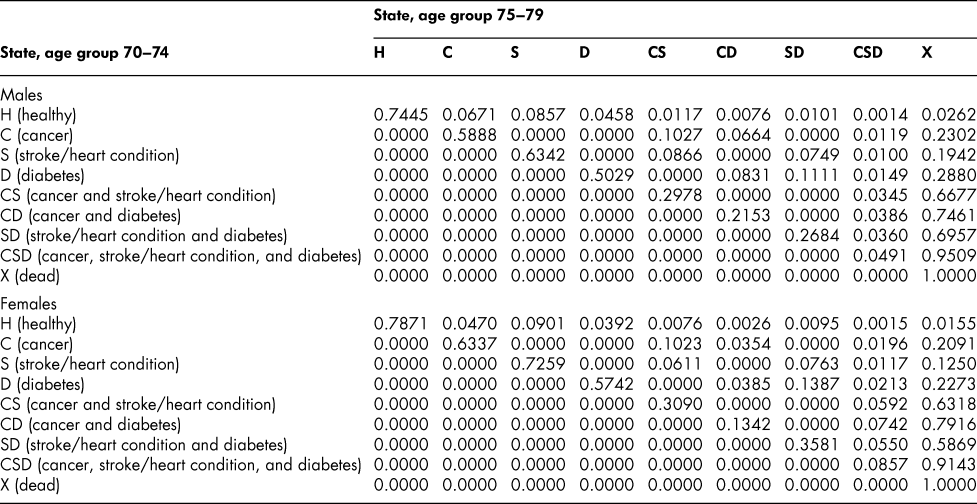
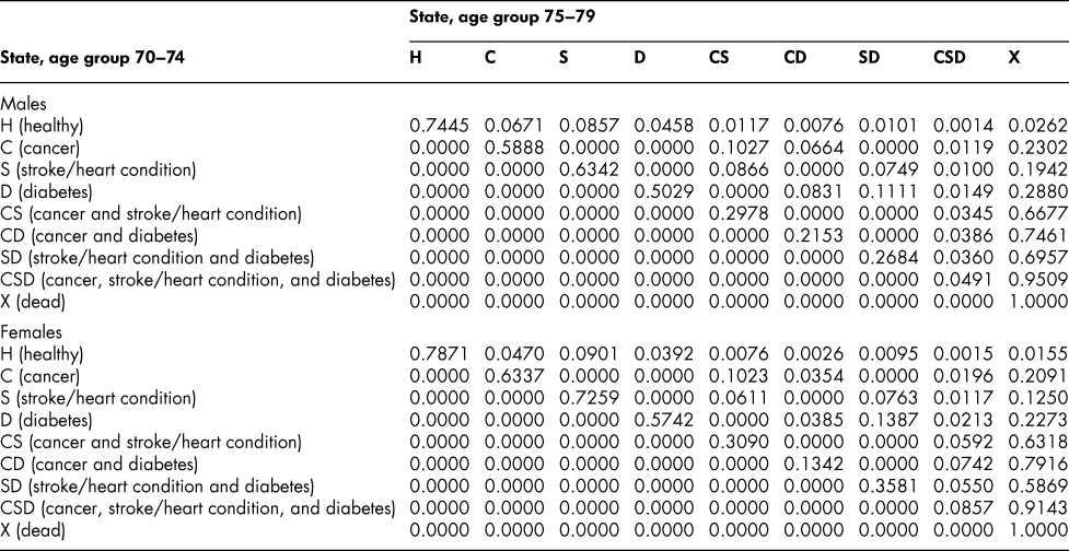
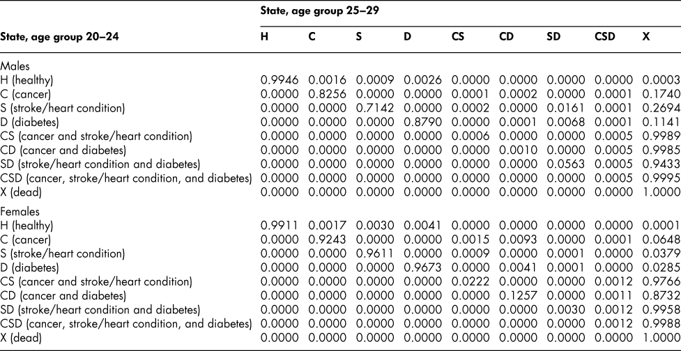
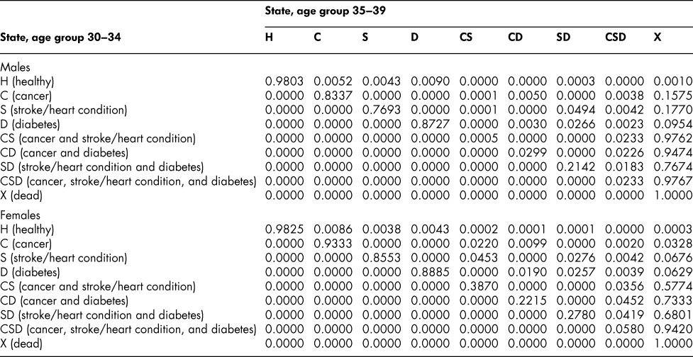
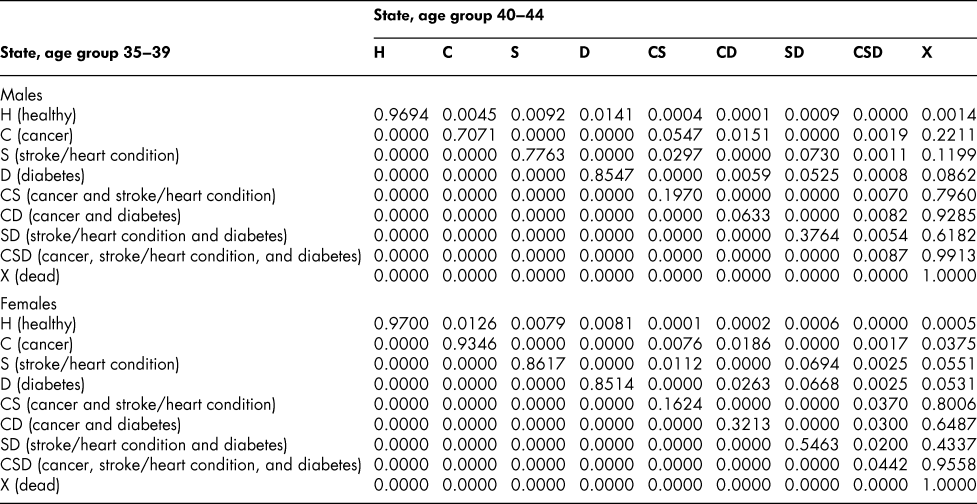
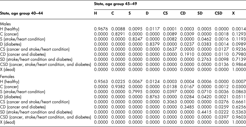
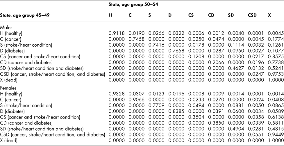
Once the flow matrix F has been derived, we calculate the transition probability matrix P as described above. Table 2 shows, for illustration, the P matrix for the 70–74 age group – the probability matrix for transitions between ages 70–74 and ages 75–79. Similar matrices for all age groups from 20–24 to 65–69 are shown in Appendix Tables A1 to A11

Table 2: State transition probabilities, age group 70–74: Basic scenario (Sc0)

The probability matrices thus constructed represent patterns of movement within an artificial population, but they are grounded in real survey and demographic data. The flow matrices on which they are based satisfy the adding-up, irreversibility, and positivity restrictions derived from the chronic conditions survey data, as they must, by construction. They satisfy also the requirement that the overall age-group-specific death probabilities must be consistent with life table probabilities, again by construction. At a more specific level: (1) the death probability for someone with two chronic conditions in Table 2 is always much higher than the single-condition probabilities (compare the probabilities for CS with those for C or S alone), and the probability for someone unlucky enough to have all three conditions is much higher still, as one would expect; (2) the death probabilities are higher for males than for females (consistent with overall life table probabilities), with the single exception of the probability for the CD state (and even there, the probability of entering that high mortality state from any other possible state is greater for males); (3) the probability of remaining in good health (staying in H) is uniformly higher for females. Overall, the probability matrices appear to pass a “reasonableness” check, both for the 70–74 age group in Table 2 and the other age groups for which we have constructed similar matrices (see Appendix), and which we have examined in detail.

Simulating the Sequence of State Vectors

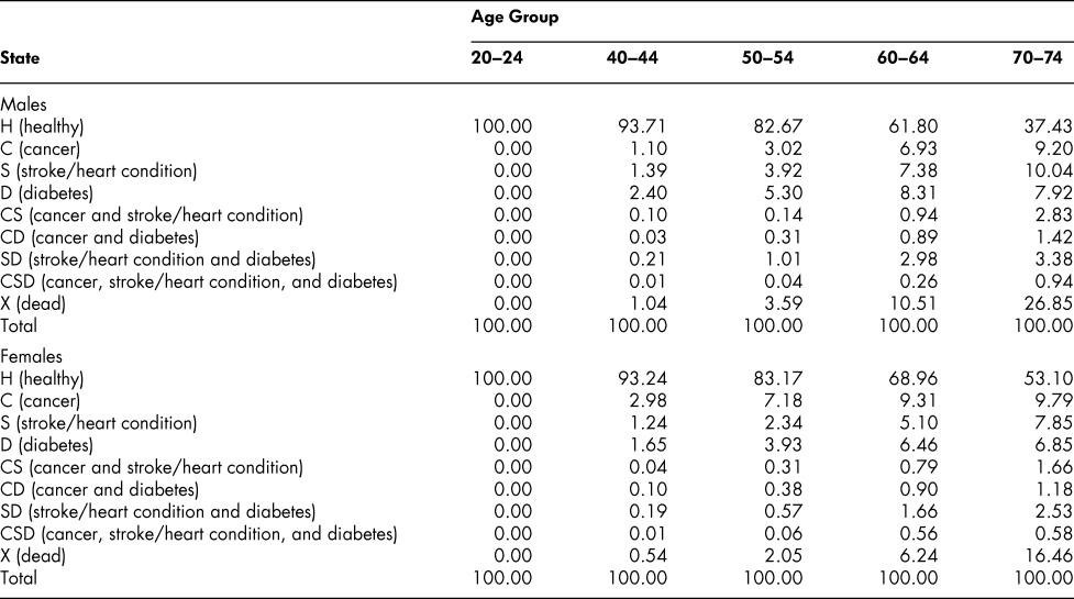
The calculated set of (male or female) transition probability matrices make it possible to simulate, recursively, the state vectors for successive age groups, starting from an assumed initial age group. We set the initial population at 100 for ages 20–24 with all members of the population assumed to be in the H state so that the initial state vector is (100, 0, 0, … , 0). (Specifying the initial vector in that form allows us the convenience of being able to interpret the elements of the subsequently calculated vectors as percentages of the original population.) We then move the initial state vector forward to ages 25–29 by applying the 20–24 transition probabilities, then to ages 30–34 by applying the 25–29 probabilities, and so on. The vectors obtained in this way are shown, for selected age groups, in Table 3.

Table 3: State vectors, selected age groups: Base scenario (Sc0)

The vector sequences in the table show that the percentage of males in good health (no C, S, or D) falls from 100 to 93.71 by ages 40–44, and then declines steadily to 37.43, by ages 70–74. For females, the percentage is almost the same as for males at ages 40–44 (93.24) but then declines more slowly; by ages 70–74, 53.10 per cent of the initial population of women are in the H state, compared with the 37.43 percentage for men.

The percentage survival rate (100 minus the percentage in the dead state) is higher for women (as we know it should be from the life tables), falling only to 83.54 per cent by ages 70–74 compared with 73.15 for men. In terms of the distribution of chronic conditions, women have a higher proportion with cancer than men at all ages after the initial one (but especially at ages below 70–74, attributable presumably to breast cancer) and lower proportions in the stroke/heart disease and diabetes categories.

A comparison indicates that the simulated percentages in Table 3 conform very closely to the percentages calculated directly from the survey data at each age, as shown in Table 4. If actual percentage distributions (state vectors) were all that were required, the whole process of developing the probability matrices might be less rewarding. However, the probabilities are of interest in themselves. Moreover, they permit alternative simulation experiments – “what if” experiments involving changing particular probabilities. Note that the simulated prevalence rates for ages 70–74 shown in Table 4 are the result of successive applications of 11 transition probability matrices, one after another, starting with ages 20–24 and covering an age space of 50 years, with no additional input of data; that differences from observed survey rates are so close to zero is for us an important and reassuring result.

Table 4: Comparison of simulated and survey percentage distribution of chronic health states: Age group 70–74

Exploration: Changing the Probabilities

Next, we alter the transition probabilities and rerun the simulations of state vectors. The altered probabilities represent nine scenarios (Sc), as we shall call them, of three different types. In the first type, the probability of developing a particular chronic condition is set to zero at all ages; the condition is thus eliminated by blocking entry into it. In the second type, the probability of developing a chronic condition is reduced by half at every age. In the third, the probability of developing a condition is unchanged but the probability of dying for someone with that condition is reduced by half at every age. Specifically the scenarios we construct are as follows:

• Sc0 – baseline scenario: no change in any of the probabilities

• ScC1 – probability of developing cancer set to zero at every age (cancer eliminated completely)

• ScC2 – probability of developing cancer reduced by half at every age

• ScC3 – probability of dying for someone with cancer reduced by half at every age

• ScS1 – probability of developing heart disease or having a stroke set to zero at every age (stroke/heart disease eliminated completely)

• ScS2 – probability of developing heart disease or having a stroke reduced by half at every age

• ScS3 – probability of dying for someone with heart disease or having a stroke reduced by half at every age

• ScD1 – probability of developing diabetes set to zero at every age (diabetes eliminated completely)

• ScD2 – probability of developing diabetes reduced by half at every age

• ScD3 – probability of dying for someone with diabetes reduced by half at every age

The adjustments to eliminate a chronic condition entirely are straightforward. To eliminate cancer, for example, the probability of entry into any state with a C label (C, CS, CD, CSD) is set to zero and the original probabilities are reassigned (the probabilities still have to sum to one in every row). C is merged with H (the original C and H probabilities are added together, that is, since no one now is able to move from H to C), CS is merged with S, CD with D, and CSD with SD, in every relevant row, leaving X unchanged. In effect, the label C disappears from the matrix.

The adjustments to reduce the chronic conditions entry probabilities by half are similar, except that half of the entry probability for a C-label state remains while the other half is merged, as explained. (Half of the probability of moving from H to C is reassigned to H, the other half remains; half of the probability of moving from S to CS is reassigned to the S-to-S probability, the other half remains as it was; and so on.)

The adjustments involving the death probabilities are trickier. Reducing the probability for someone in the C state is straightforward, for example – the probability of moving from C to CX in the C row of the matrix is simply half of what it was originally and the difference reassigned pro rata to the other probabilities in that row. But how to alter the probabilities in a row such as the CD row require some assumption. Presumably, the death probability for someone with both cancer and diabetes should be lowered if the death probability for someone with cancer alone are lowered, but by how much? Our working assumption is that the new death probability for someone in the CD state should be adjusted by a factor equal to the death probability for D alone plus the reduced death probability for C alone, divided by the original sum of the same two probabilities. That assumption takes into account the relationship between the C and D probabilities in adjusting the death probability for the combined CD state. The CD death probability having been thus reduced, the difference from the original probability is then reassigned to the other nonzero probabilities in the CD row. Similar assumptions are made for the other combined-state probabilities in the matrix.

Interpreting the Scenario Simulations

The simulated state vectors corresponding to the altered probability scenarios are shown in Table 5 for the 70–74 male and female age groups, generated, as before, from an initial 100 per cent healthy age 20–24 vector. Eliminating cancer increases markedly the proportion of 70–74-year-olds in the healthy state, as one would expect, and raises the proportion of survivors – from 73.15 to 79.61 for males, 83.54 to 90.18 for females. But with more survivors, free of cancer, but eligible for the other chronic conditions, the stroke/heart disease and diabetes proportions increase, both separately and in combination. Reducing the cancer entry probability by only half at every age (ScC2) has similar but correspondingly smaller effects on the state vectors. Eliminating or reducing the entry probabilities for stroke/heart disease and diabetes (ScS1, ScS2, ScD1, ScD2) increases the proportion in the healthy state and the proportion of survivors in a similar way, but with some differences in size of effect, and increases also the proportions with the other chronic conditions. Interestingly, though, cutting the death probability by half for a particular chronic condition (ScC3, ScS3, ScD3) has a smaller effect than cutting the entry probability by half. Cutting the cancer entry probability by half at every age, for example, increases the ages 70–74 survival proportion from 73.15 to 76.28 for males but reducing the death probability at every age by half increases it only to 75.32, as shown in Table 6. For females, the corresponding changes are from 83.54 to 86.73 with the entry probability reductions, but only to 85.56 with the death probability reductions.

Table 5: State vectors, ages 20–24 and 70–74: Alternative scenarios

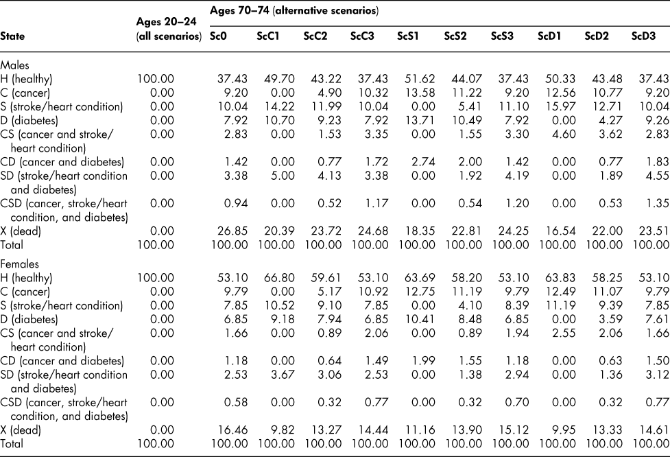
Table 6: Percentages of survivors at selected older ages: Alternative scenarios

These results reflect the complex system of interactions among the different chronic conditions and mortality probabilities. Someone living longer because of a reduced probability of developing one of the conditions has an increased probability of developing one or both of the other conditions over his/her lifetime, with concomitant changes in death probabilities. An advantage of modelling different chronic conditions and mortality rates together in a single integrated age-dynamic system is that it brings to light and takes account of these interactions. (We refer here to the system as age-dynamic because it allows the effects of state changes in one age group to carry forward to subsequent ages as the group grows older. From the point of view of the entire population, though, the system is stationary: the probabilities at any given age are invariant with time.) That there are such interactions is not a novel idea: it is well known in the literature on modelling the effects of eliminating cancer or other particular diseases. Our contribution is to make it explicit in an integrated framework, to show how the interactions play out from youth to old age, and to show how the associated “what if” probabilities can be derived by experimenting with a model constructed from life table and chronic conditions survey data.

Some Implications for Health Care Utilization

The survey that provide our chronic conditions data provides also some information on four types of health care services – the annual numbers of overnight stays in hospital, family doctor consultations, eye specialist consultations, and other medical doctor consultations. The numbers can be converted to age-group-specific per capita utilization ratios for the population in different chronic conditions categories and incorporated into our framework. We apply the ratios to each of the eight living-population states and aggregate the results to obtain overall indexes for the four types of health care services, with the Sc0 scenario index set at a base value of 100.0. Table 7 shows how the indexes differ from that value in the other scenarios.

Table 7: Utilization of hospital and medical services: Alternative scenarios (indexes: Sc0 = 100.0)

Note: Hospital services are based on annual numbers of overnight stays; other services are based on annual numbers of consultations.

We note a few of the features of the table and offer some interpretation. First, in general, there are two types of effects. Eliminating or reducing the incidence of a chronic condition results in less use of the particular services required for dealing with that condition. Thus, eliminating or reducing the incidence of cancer results in a lowering of the population’s aggregate number of nights in hospital and the aggregate use of the services of relevant medical specialists (caught up in the “other medical doctor” category). That is one type of effect. The other type is the effect of simply prolonging lives, as reflected most prominently in the ScC3, ScS3, and ScD3 scenarios: cutting the death probabilities for a particular chronic condition means more people living, and using a range of health care services (like the rest of the population) at any given time. More living elderly people means more use of eye specialist services, for example. These two effects do not operate independently, of course; reducing the probability of getting cancer would no doubt have both of them, although the first one seems to dominate. The biggest effects of all in the table come from the elimination or reduction in the stroke/heart condition category: hospital utilization declines by 17 or 18 per cent in ScS1 and 8 per cent in ScS2, for both males and females.

The foregoing is our interpretation of the results in Table 7. We do not want to read too much into them; they represent a high level of aggregation and a simplification of what is no doubt a complex set of interactions within the health care system. However, they do serve to draw attention to the two types of effects that one might expect from improvements in treatment and mortality reduction – the direct effects on the utilization of particular services for a given condition and the indirect effects that come about simply from having more people living longer lives.