


1 Introduction
1.1 Definitions and state of the art
For a (smooth) function
 $E(x_1,\ldots ,x_n)$
, the Hessian
$E(x_1,\ldots ,x_n)$
, the Hessian
 ${\textrm {d}}^2 E= \left ( \frac {\partial ^2 E}{\partial x_i \partial x_j}\right )$
is a symmetric bilinear form. If it is positive definite, it defines a Riemannian metric called the Hessian metric. Although the construction strongly depends on the coordinate system, Hessian metrics naturally appear in many subjects of mathematics.
${\textrm {d}}^2 E= \left ( \frac {\partial ^2 E}{\partial x_i \partial x_j}\right )$
is a symmetric bilinear form. If it is positive definite, it defines a Riemannian metric called the Hessian metric. Although the construction strongly depends on the coordinate system, Hessian metrics naturally appear in many subjects of mathematics.
For example, for toric Kähler manifolds, the metrics on the quotient space are (locally) Hessian metrics. Metrics admitting nontrivial geodesic equivalence are also Hessian metrics (see, e.g., [Reference Bolsinov, Matveev and Rosemann13, Section 4.2]). There is a strong relation between Hessian metrics and the Hamiltonian construction in the theory of infinite-dimensional integrable system of hydrodynamic type (see, e.g., [Reference Bolsinov, Konyaev and Matveev12, Reference Gelfand and Ja25]). Hessian metrics naturally come in many geometric constructions of Riemannian metrics inside convex domains (see, e.g., [Reference Cheng and Yau16]), in affine geometry of hypersurfaces (see, e.g., [Reference Laugwitz32, Reference Li, Simon, Zhao and Hu33]) and in information geometry (see, e.g., [Reference Shima, Nielsen and Barbaresco48]). We refer to [Reference Shima47] for a comprehensive study of differential geometry of Hessian metrics and their applications.
We are interested in Hessian metrics that naturally appear in convex and Finsler geometry. They are defined on
 $\mathbb {R}^n \setminus {\{0\}}$
, and the function E satisfies the following restriction: it is positively 2-homogeneous, that is, for any
$\mathbb {R}^n \setminus {\{0\}}$
, and the function E satisfies the following restriction: it is positively 2-homogeneous, that is, for any
 $\lambda>0$
, we have
$\lambda>0$
, we have
 $E(\lambda y)= \lambda ^2 E(y)$
.
$E(\lambda y)= \lambda ^2 E(y)$
.
Under this assumption, the function E defines a Minkowski norm
 $F:= \sqrt { 2 E}$
on
$F:= \sqrt { 2 E}$
on
 $\mathbb {R}^n$
, i.e., F satisfies positiveness and smoothness on
$\mathbb {R}^n$
, i.e., F satisfies positiveness and smoothness on
 $\mathbb {R}^n\backslash \{0\}$
, positive 1-homogeneity (i.e.,
$\mathbb {R}^n\backslash \{0\}$
, positive 1-homogeneity (i.e.,
 $F(\lambda y)= \lambda F(y)$
for
$F(\lambda y)= \lambda F(y)$
for
 $\lambda> 0$
), and strong convexity (i.e.,
$\lambda> 0$
), and strong convexity (i.e.,
 ${\textrm {d}}^2E=\tfrac 12{\textrm {d}}^2 (F^2)$
is positive definite on
${\textrm {d}}^2E=\tfrac 12{\textrm {d}}^2 (F^2)$
is positive definite on
 $\mathbb {R}^n\backslash \{0\}$
). Notice that the strong convexity implies the triangle inequality (i.e.,
$\mathbb {R}^n\backslash \{0\}$
). Notice that the strong convexity implies the triangle inequality (i.e.,
 $F( y_1 + y_2) \le F( y_1) + F( y_2)$
,
$F( y_1 + y_2) \le F( y_1) + F( y_2)$
,
 $\forall y_1,y_2\in \mathbb {R}^n$
) and the convexity (i.e.,
$\forall y_1,y_2\in \mathbb {R}^n$
) and the convexity (i.e.,
 $F( \lambda y_1 + (1-\lambda )y_2) \le \lambda F( y_1) + (1-\lambda )F( y_2)$
,
$F( \lambda y_1 + (1-\lambda )y_2) \le \lambda F( y_1) + (1-\lambda )F( y_2)$
,
 $\forall y_1,y_2\in \mathbb {R}^n,\lambda \in [0,1]$
) in the usual sense.
$\forall y_1,y_2\in \mathbb {R}^n,\lambda \in [0,1]$
) in the usual sense.
It is known that the indicatrix
 $S_F$
determines the Minkowski norm F and (as we recall below) that the Hessian metric of
$S_F$
determines the Minkowski norm F and (as we recall below) that the Hessian metric of
 $E= \tfrac {1}{2} F^2 $
determines the function E. So the study of strongly convex bodies with smooth boundary can be reduced to the study of Hessian metrics for
$E= \tfrac {1}{2} F^2 $
determines the function E. So the study of strongly convex bodies with smooth boundary can be reduced to the study of Hessian metrics for
 $E= \tfrac {1}{2} F^2$
and, in particular, apply methods and results of Riemannian geometry. We refer to [Reference Laugwitz32, Reference Schneider43] for more details on the interrelation between Hessian geometry and convex geometry. In a latter discussion, we will reserve the notation F for the Minkowski norm and
$E= \tfrac {1}{2} F^2$
and, in particular, apply methods and results of Riemannian geometry. We refer to [Reference Laugwitz32, Reference Schneider43] for more details on the interrelation between Hessian geometry and convex geometry. In a latter discussion, we will reserve the notation F for the Minkowski norm and
 $E= \frac {1}{2} F^2 $
for the function we use to build a Hessian metric.
$E= \frac {1}{2} F^2 $
for the function we use to build a Hessian metric.
The appearance of Hessian metrics in Finsler geometry is related to that in the convex geometry. Recall that a Finsler metric on a smooth manifold M with
 $\operatorname {dim} M> 1$
is a continuous function F on
$\operatorname {dim} M> 1$
is a continuous function F on
 $TM$
such that it is smooth on the slit tangent bundle
$TM$
such that it is smooth on the slit tangent bundle
 $TM \setminus \{ 0\} $
and such that its restriction to each tangent space
$TM \setminus \{ 0\} $
and such that its restriction to each tangent space
 $T_pM$
is a Minkowski norm. The corresponding Hessian metric g is then a Riemannian metric on the slit tangent space
$T_pM$
is a Minkowski norm. The corresponding Hessian metric g is then a Riemannian metric on the slit tangent space
 $T_pM\setminus \{0\}$
. It was called the fundamental tensor by Berwald [Reference Berwald9], and it naturally comes to many geometric constructions in Finsler geometry.
$T_pM\setminus \{0\}$
. It was called the fundamental tensor by Berwald [Reference Berwald9], and it naturally comes to many geometric constructions in Finsler geometry.
In this paper, we study isometries between the Hessian metrics of Minkowski norms. We call the diffeomorphism
 $\Phi :\mathbb {R}^n\backslash \{0\} \rightarrow \mathbb {R}^n\backslash \{0\}$
a Hessian isometry from
$\Phi :\mathbb {R}^n\backslash \{0\} \rightarrow \mathbb {R}^n\backslash \{0\}$
a Hessian isometry from
 $F_1$
to
$F_1$
to
 $F_2$
, if it is an isometry between the Hessian metrics
$F_2$
, if it is an isometry between the Hessian metrics
 $g_1= {\textrm {d}}^2 E_1= \tfrac {1}2 {\textrm {d}}^2 (F_1^2)$
and
$g_1= {\textrm {d}}^2 E_1= \tfrac {1}2 {\textrm {d}}^2 (F_1^2)$
and
 $g_2= {\textrm {d}}^2 E_2= \tfrac {1}2 {\textrm {d}}^2 (F_2^2)$
. By local Hessian isometry, we understand a positively 1-homogeneous diffeomorphism between two conic domains that is isometry with respect to the restriction of the Hessian metrics to these domains. Here, the positive 1-homogeneity for the local Hessian isometry
$g_2= {\textrm {d}}^2 E_2= \tfrac {1}2 {\textrm {d}}^2 (F_2^2)$
. By local Hessian isometry, we understand a positively 1-homogeneous diffeomorphism between two conic domains that is isometry with respect to the restriction of the Hessian metrics to these domains. Here, the positive 1-homogeneity for the local Hessian isometry
 $\Phi $
is the property that
$\Phi $
is the property that
 $\Phi (\lambda x)=\lambda \Phi (x)$
for any
$\Phi (\lambda x)=\lambda \Phi (x)$
for any
 $\lambda>0$
and any
$\lambda>0$
and any
 $x\in \mathbb {R}^n\backslash \{0\}$
where
$x\in \mathbb {R}^n\backslash \{0\}$
where
 $\Phi $
is defined. By conic domain, we understand
$\Phi $
is defined. By conic domain, we understand
 $$ \begin{align*}C(U):= \{\lambda y \ \mid \ y \in U \ , \ \lambda>0\}, \text{where}\ U\subset \mathbb{R}^n\backslash\{0\}. \end{align*} $$
Let us recall some known facts (e.g., [Reference Bao, Chern and Shen8, Reference Laugwitz32]) that follow from the positive 1-homogeneity of F.
-
• The Hessian metric determines geometrically the “radial” rays, i.e., the sets of the form
 $\{t y \mid t\in \mathbb {R}_{>0}\}$
, with nonzero y. Indeed, these rays are geodesics for the Hessian metrics, and are precisely those which are not complete.
$\{t y \mid t\in \mathbb {R}_{>0}\}$
, with nonzero y. Indeed, these rays are geodesics for the Hessian metrics, and are precisely those which are not complete. -
• The Hessian metric
$g={\textrm {d}}^2E$
determines the functions E and F by
$F(y)^2= g(y,y)$
for every
$y\in \mathbb {R}^n\backslash \{0\}$
. -
• The Hessian metric g is the cone metric over its restriction to the indicatrix
$S_F$
, i.e.,
$g=({\textrm {d}}F)^2+F^2 g_{|S_F}$
. That is, in any local coordinate system
$(r,\xi _2,\ldots ,\xi _{n})$
such that
$F(r,\xi _2,\ldots ,\xi _n)= r$
, we have
$g= dr^2 + r^2 \sum _{i,j=2}^{n} h_{ij}d\xi _id\xi _j$
, where the components
$h_{ij}$
do not depend on r.


These three observations imply that any Hessian isometry
 $\Phi $
from
$\Phi $
from
 $F_1$
to
$F_1$
to
 $F_2$
satisfies the positive 1-homogeneity and diffeomorphically maps the indicatrix
$F_2$
satisfies the positive 1-homogeneity and diffeomorphically maps the indicatrix
 $S_{F_1}$
to
$S_{F_1}$
to
 $S_{F_2}$
. Any local Hessian isometry
$S_{F_2}$
. Any local Hessian isometry
 $\Phi :C(U_1)\to C(U_2)$
is 1-homogeneous by definition and diffeomorphically maps
$\Phi :C(U_1)\to C(U_2)$
is 1-homogeneous by definition and diffeomorphically maps
 $S_{F_1}\cap C(U_1)$
to
$S_{F_1}\cap C(U_1)$
to
 $S_{F_2}\cap C(U_2)$
.
$S_{F_2}\cap C(U_2)$
.
Moreover, a positively 1-homogeneous mapping
 $\Phi $
which maps
$\Phi $
which maps
 $S_{F_1}$
to
$S_{F_1}$
to
 $S_{F_2}$
is a Hessian isometry if and only if its restriction to
$S_{F_2}$
is a Hessian isometry if and only if its restriction to
 $S_{F_1}$
is an isometry between
$S_{F_1}$
is an isometry between
 ${g_i}_{|S_{F_i}}$
.
${g_i}_{|S_{F_i}}$
.
Let us now recall some known examples of Hessian isometries.
If
 $\Phi :\mathbb {R}^n \to \mathbb {R}^n $
is a linear isomorphism and
$\Phi :\mathbb {R}^n \to \mathbb {R}^n $
is a linear isomorphism and
 $\Phi ^* F_2 =F_2\circ \Phi =F_1$
, then
$\Phi ^* F_2 =F_2\circ \Phi =F_1$
, then
 $\Phi $
is trivially a Hessian isometry from
$\Phi $
is trivially a Hessian isometry from
 $F_1$
to
$F_1$
to
 $F_2$
. Indeed, for any linear coordinate change, the Hessian metric
$F_2$
. Indeed, for any linear coordinate change, the Hessian metric
 $g= \tfrac {1}{2}{\textrm {d}}^2 (F^2)$
is covariant by the Leibnitz formula. Such isometries will be called linear isometries.
$g= \tfrac {1}{2}{\textrm {d}}^2 (F^2)$
is covariant by the Leibnitz formula. Such isometries will be called linear isometries.
Suppose dimension
 $n=2$
. This case is completely understood, and there are many examples of nonlinear Hessian isometries. To see this, let us consider the so-called generalized polar coordinates on
$n=2$
. This case is completely understood, and there are many examples of nonlinear Hessian isometries. To see this, let us consider the so-called generalized polar coordinates on
 $\mathbb {R}^2 \setminus \{0\}$
. This coordinate system is a special case of the cone coordinate system discussed above. It is constructed as follows: the first coordinate is simply F, so the indicatrix of F is the coordinate line corresponding to the value
$\mathbb {R}^2 \setminus \{0\}$
. This coordinate system is a special case of the cone coordinate system discussed above. It is constructed as follows: the first coordinate is simply F, so the indicatrix of F is the coordinate line corresponding to the value
 $1$
. Next, on the indicatrix (which is a closed convex simple curve) we denote by
$1$
. Next, on the indicatrix (which is a closed convex simple curve) we denote by
 $\theta $
the arc-length parameter corresponding to the Hessian metrics g. For each
$\theta $
the arc-length parameter corresponding to the Hessian metrics g. For each
 $y= (x_1,x_2)\in \mathbb {R}^2 \setminus \{0\}$
, its
$y= (x_1,x_2)\in \mathbb {R}^2 \setminus \{0\}$
, its
 $\theta $
-coordinate is that for
$\theta $
-coordinate is that for
 $\tfrac {1}{F(y)} y\in S_F$
. See Figure 1.
$\tfrac {1}{F(y)} y\in S_F$
. See Figure 1.

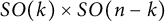
Figure 1: Generalised polar coordinates
 $(F, \theta )$
: first coordinate lines are
$(F, \theta )$
: first coordinate lines are
 $\{F= \text{const}\}$
, and second coordinate lines are rays from zero. The second coordinate is chosen such that on
$\{F= \text{const}\}$
, and second coordinate lines are rays from zero. The second coordinate is chosen such that on
 $\{F=1\}$
it corresponds to the g-arclength parameter.
$\{F=1\}$
it corresponds to the g-arclength parameter.
If
 $E=\tfrac {1}{2} (x_1^2 + x_2^2)$
(so that
$E=\tfrac {1}{2} (x_1^2 + x_2^2)$
(so that
 $g= dx_1^2 + dx_2^2$
), generalized polar coordinates are the usual polar coordinates. In the general case,
$g= dx_1^2 + dx_2^2$
), generalized polar coordinates are the usual polar coordinates. In the general case,
 $\theta $
is still periodic and is defined up to addition of a constant to
$\theta $
is still periodic and is defined up to addition of a constant to
 $\theta $
and the change of the sign, but the period is not necessary
$\theta $
and the change of the sign, but the period is not necessary
 $2\pi $
.
$2\pi $
.
In the generalized polar coordinates, the Hessian metric
 $g= \tfrac {1}{2}{\textrm {d}}^2 (F^2)= {\textrm {d}}F^2 + F^2 d\theta ^2 $
is flat. So we see that any two 2-dimensional Minkowski norms are locally Hessian-isometric, and are Hessian-isometric if and only if their indicatrices have the same length in the corresponding Hessian metrics.
$g= \tfrac {1}{2}{\textrm {d}}^2 (F^2)= {\textrm {d}}F^2 + F^2 d\theta ^2 $
is flat. So we see that any two 2-dimensional Minkowski norms are locally Hessian-isometric, and are Hessian-isometric if and only if their indicatrices have the same length in the corresponding Hessian metrics.
Let us now consider
 $n\ge 3$
. This case is almost completely open: in the literature, we found one nonlinear example of Hessian isometry, which we will recall and generalize later, and one negative result, which is the following theorem.
$n\ge 3$
. This case is almost completely open: in the literature, we found one nonlinear example of Hessian isometry, which we will recall and generalize later, and one negative result, which is the following theorem.
Theorem 1.1 ([Reference Brickell14]; for alternative proof, see [Reference Schneider42])
Let F be a Minkowski norm on
 $\mathbb {R}^n$
,
$\mathbb {R}^n$
,
 $n\ge 3$
. Assume it is absolutely homogeneous, that is,
$n\ge 3$
. Assume it is absolutely homogeneous, that is,
 $F(\lambda y)=|\lambda |\cdot F(y)$
for every
$F(\lambda y)=|\lambda |\cdot F(y)$
for every
 $\lambda \in \mathbb {R}$
and
$\lambda \in \mathbb {R}$
and
 $y\in \mathbb {R}^n$
.
$y\in \mathbb {R}^n$
.
Then, if the Hessian metric
 $g= \tfrac {1}{2}{\textrm {d}}^2 (F^2)$
on
$g= \tfrac {1}{2}{\textrm {d}}^2 (F^2)$
on
 $\mathbb {R}^n\backslash \{0\}$
has zero curvature, F is euclidean, that is,
$\mathbb {R}^n\backslash \{0\}$
has zero curvature, F is euclidean, that is,
 $F= {\sqrt { \sum _{i,j} \alpha _{ij} x_i x_j}}$
for a positive definite symmetric matrix
$F= {\sqrt { \sum _{i,j} \alpha _{ij} x_i x_j}}$
for a positive definite symmetric matrix
 $(\alpha _{ij})\in \mathbb {R}^{n\times n}$
. In this case, every Hessian isometry is linear.
$(\alpha _{ij})\in \mathbb {R}^{n\times n}$
. In this case, every Hessian isometry is linear.
The proofs in [Reference Brickell14, Reference Schneider42] are different, but the assumption that F is absolutely homogeneous is essential for both.
Let us now recall and slightly generalize the only known example of nonlinear Hessian isometry in dimension
 $n\ge 3$
. We start with any Minkowski norm F on the space
$n\ge 3$
. We start with any Minkowski norm F on the space
 $\mathbb {R}^n$
of column vectors, set
$\mathbb {R}^n$
of column vectors, set
 $E=\tfrac {1}{2}F^2$
, and consider the corresponding Legendre transformation:
$E=\tfrac {1}{2}F^2$
, and consider the corresponding Legendre transformation:
 $$ \begin{align} \Phi: \mathbb{R}^n\setminus \{0\} \to \mathbb{R}^n\setminus\{0\}\ , \ \ y= (x_1,\ldots,x_n)^T\mapsto \left( \tfrac{\partial}{\partial x_1}E(y),\ldots, \tfrac{\partial}{\partial x_n}E(y)\right)^T. \end{align} $$
For the euclidean Minkowski norm
 $F=\sqrt {x_1^2+\cdots +x_n^2} $
, the Legendre transformation
$F=\sqrt {x_1^2+\cdots +x_n^2} $
, the Legendre transformation
 $\Phi = \text {id}$
.
$\Phi = \text {id}$
.
Obviously, the function
 $\hat E=\Phi _*(E)$
on
$\hat E=\Phi _*(E)$
on
 $\mathbb {R}^n\backslash \{0\}$
is a positive smooth function satisfying the positive 2-homogeneity. As we explain below in Remark 1.2 (see also [Reference Bao, Chern and Shen8, Section 4.8]), the Hessian of
$\mathbb {R}^n\backslash \{0\}$
is a positive smooth function satisfying the positive 2-homogeneity. As we explain below in Remark 1.2 (see also [Reference Bao, Chern and Shen8, Section 4.8]), the Hessian of
 $\hat E$
is given by the matrix inverse to that for g and is therefore positive definite. Then,
$\hat E$
is given by the matrix inverse to that for g and is therefore positive definite. Then,
 $ \hat F= \sqrt { 2\hat E}$
is a Minkowski norm.
$ \hat F= \sqrt { 2\hat E}$
is a Minkowski norm.
In [Reference Schneider43], it was proved that the Legendre transformation
 $\Phi $
in (1.1) is a Hessian isometry from F to
$\Phi $
in (1.1) is a Hessian isometry from F to
 $\hat F$
. Clearly, it is linear if and only if F is euclidean.
$\hat F$
. Clearly, it is linear if and only if F is euclidean.
Remark 1.2 Schneider’s observation that the Legendre transformation
 $\Phi $
in (1.1) is a Hessian isometry is important for our paper, so let us sketch a proof. Using
$\Phi $
in (1.1) is a Hessian isometry is important for our paper, so let us sketch a proof. Using
 $g_{ij}=\tfrac {\partial ^2 E}{\partial x_i\partial x_j}$
for the Hessian metric of F and the explained above formula
$g_{ij}=\tfrac {\partial ^2 E}{\partial x_i\partial x_j}$
for the Hessian metric of F and the explained above formula
 $E= \tfrac {1}{2} \sum _{i,j}g_{ij} x_i x_j$
, the Legendre transformation
$E= \tfrac {1}{2} \sum _{i,j}g_{ij} x_i x_j$
, the Legendre transformation
 $\Phi $
in (1.1) can be presented at
$\Phi $
in (1.1) can be presented at
 $y=(x_1,\ldots ,x_n)^T\in \mathbb {R}^n\backslash \{0\}$
as (see, e.g., [Reference Bao, Chern and Shen8, equation (14.8.1)])
$y=(x_1,\ldots ,x_n)^T\in \mathbb {R}^n\backslash \{0\}$
as (see, e.g., [Reference Bao, Chern and Shen8, equation (14.8.1)])
 $$ \begin{align*} \Phi(y)=\left(\tfrac{\partial}{\partial x_j}\tfrac{1}{2}\sum_{i,k} g_{ik} x_i x_k\right)_{1\leq j\leq n}\!\!=\left(\sum_{i} g_{ij} x_i + \tfrac{1}{2}\sum_{i, k} \tfrac{\partial g_{ik}}{\partial x_j}x_ix_k \right)_{1\leq j\leq n}\!\!=\left(\sum_{i} g_{ij} x_i \right)_{1\leq j\leq n}. \end{align*} $$
Here, we have used
 $\sum _i\tfrac {\partial g_{ik}}{\partial x_j}x_ix_k=x_k\left (\sum _i\tfrac {\partial g_{ik}}{\partial x_j}x_i\right )=0$
by the positive
$\sum _i\tfrac {\partial g_{ik}}{\partial x_j}x_ix_k=x_k\left (\sum _i\tfrac {\partial g_{ik}}{\partial x_j}x_i\right )=0$
by the positive
 $2$
-homogeneity of E. Then, its differential
$2$
-homogeneity of E. Then, its differential
 $d\Phi $
at y has the Jacobi matrix
$d\Phi $
at y has the Jacobi matrix
 $$ \begin{align*} \left(d\Phi \right)_{1\leq i,j\leq n} = \left( g_{ij} + \sum_{k} \tfrac{\partial g_{ik}}{\partial x_j} x_k \right)_{1\leq i,j\leq n} = \left(g_{ij}\right)_{1\leq i,j\leq n}. \end{align*} $$
Because the Legendre transformation is an involution, and
 $\Phi ^{-1}$
is the Legendre transformation in (1.1) with
$\Phi ^{-1}$
is the Legendre transformation in (1.1) with
 $F=\hat {\hat {F}}$
and
$F=\hat {\hat {F}}$
and
 $\hat F$
exchanged, the Hessian metric
$\hat F$
exchanged, the Hessian metric
 $\hat g$
for
$\hat g$
for
 $\hat F$
at
$\hat F$
at
 $\Phi (x)$
is represented by the inverse matrix
$\Phi (x)$
is represented by the inverse matrix
 $(g^{ij})_{1\leq i,j\leq n}$
for F at x (see [Reference Bao, Chern and Shen8, Proposition 14.8.1] for more details). So the pullback
$(g^{ij})_{1\leq i,j\leq n}$
for F at x (see [Reference Bao, Chern and Shen8, Proposition 14.8.1] for more details). So the pullback
 $\Phi ^* \hat {g}$
is given by the matrix
$\Phi ^* \hat {g}$
is given by the matrix
 $$ \begin{align*}\left(\sum_{s,r} g^{sr} g_{si} g_{rj}\right)_{1\leq i,j\leq n} =\left( g_{ij}\right)_{1\leq i,j\leq n}, \end{align*} $$
which is the matrix of the Hessian metric g for F.
Let us now modify the above example. We start with the euclidean Minkowski norm
 $F_0= \sqrt {x_1^2+\cdots +x_n^2}$
, and slightly deform it on two conic open subsets
$F_0= \sqrt {x_1^2+\cdots +x_n^2}$
, and slightly deform it on two conic open subsets
 $C(U_1)$
and
$C(U_1)$
and
 $C(U_2)$
of
$C(U_2)$
of
 $\mathbb {R}^n\backslash \{0\}$
, where
$\mathbb {R}^n\backslash \{0\}$
, where
 $U_1$
and
$U_1$
and
 $U_2$
are two open subsets of
$U_2$
are two open subsets of
 $S_{F_0}$
with disjoint closures. We obtain a new Minkowski norm
$S_{F_0}$
with disjoint closures. We obtain a new Minkowski norm
 $F_1$
. Denote by
$F_1$
. Denote by
 $\Phi $
the Legendre transformation and by
$\Phi $
the Legendre transformation and by
 $\hat {F}_1$
the push-forward of
$\hat {F}_1$
the push-forward of
 $F_1$
(see Figure 2). The second new Minkowski norm
$F_1$
(see Figure 2). The second new Minkowski norm
 $F_2$
is constructed as follows: it coincides with
$F_2$
is constructed as follows: it coincides with
 $\hat {F}_1$
on
$\hat {F}_1$
on
 $C(U_2)$
and with
$C(U_2)$
and with
 $F_1$
on
$F_1$
on
 $\mathbb {R}^n\backslash C(U_2)$
. It is still a smooth strictly convex Minkowski norm. Next, we consider the mapping
$\mathbb {R}^n\backslash C(U_2)$
. It is still a smooth strictly convex Minkowski norm. Next, we consider the mapping
 $\tilde \Phi $
such that it is identity on
$\tilde \Phi $
such that it is identity on
 $C(U_1)$
and
$C(U_1)$
and
 $\Phi $
on
$\Phi $
on
 $\mathbb {R}^n\backslash C(U_1)$
. It is a Hessian isometry from
$\mathbb {R}^n\backslash C(U_1)$
. It is a Hessian isometry from
 $F_1$
to
$F_1$
to
 $F_2$
. If
$F_2$
. If
 $F_1$
is different from
$F_1$
is different from
 $F_0$
on both
$F_0$
on both
 $C(U_1)$
and
$C(U_1)$
and
 $C(U_2)$
,
$C(U_2)$
,
 $\tilde {\Phi }$
is neither a linear isometry nor a Legendre transform.
$\tilde {\Phi }$
is neither a linear isometry nor a Legendre transform.

Figure 2: Construction of nonlinear and non-Legendre Hessian isometry: the function
 $E_1=E$
is different from
$E_1=E$
is different from
 $x_1^2+\cdots +x_n^2$
in cones over
$x_1^2+\cdots +x_n^2$
in cones over
 $U_1$
and
$U_1$
and
 $U_2$
(gray triangles). The function
$U_2$
(gray triangles). The function
 $\hat E$
(second picture) is the Legendre-transform of
$\hat E$
(second picture) is the Legendre-transform of
 $E=E_1$
. The function
$E=E_1$
. The function
 $E_2$
coincides with
$E_2$
coincides with
 $E_1$
everywhere, but in
$E_1$
everywhere, but in
 $C(U_2)$
and in
$C(U_2)$
and in
 $C(U_2)$
, it coincides with
$C(U_2)$
, it coincides with
 $\hat E$
.
$\hat E$
.
One can build this example such that
 $F_1$
and
$F_1$
and
 $F_2$
are preserved by the standard block diagonal action of
$F_2$
are preserved by the standard block diagonal action of
 $O(k)\times O(n-k)$
(of course, in this case, the conic open sets
$O(k)\times O(n-k)$
(of course, in this case, the conic open sets
 $C(U_i)$
must be
$C(U_i)$
must be
 $O(k)\times O(n-k)$
-invariant). One can impose additional symmetries on the construction, so the resulting metric
$O(k)\times O(n-k)$
-invariant). One can impose additional symmetries on the construction, so the resulting metric
 $F_2$
has, in addition to this linear
$F_2$
has, in addition to this linear
 $O(k)\times O(n-k)$
-symmetry, a nonlinear Hessian self-isometry. One can further generalize this example by starting with
$O(k)\times O(n-k)$
-symmetry, a nonlinear Hessian self-isometry. One can further generalize this example by starting with
 $F_0$
which is not euclidean but still has “euclidean pieces” and by deforming
$F_0$
which is not euclidean but still has “euclidean pieces” and by deforming
 $F_0$
in more than two (even infinitely many) open subsets.
$F_0$
in more than two (even infinitely many) open subsets.
1.2 Results
We consider a Minkowski norm F on
 $\mathbb {R}^n$
with
$\mathbb {R}^n$
with
 $n\geq 3$
which has a linear
$n\geq 3$
which has a linear
 $SO(k)\times SO(n-k)$
-symmetry, and study connected isometry group (i.e., the identity component of the group of all isometries) of the Hessian metric of F. We prove:
$SO(k)\times SO(n-k)$
-symmetry, and study connected isometry group (i.e., the identity component of the group of all isometries) of the Hessian metric of F. We prove:
Theorem 1.3 Suppose F is a Minkowski norm on
 $\mathbb {R}^n$
with
$\mathbb {R}^n$
with
 $n\geq 3$
, which is invariant with respect to the standard block diagonal action of the group
$n\geq 3$
, which is invariant with respect to the standard block diagonal action of the group
 $SO(k)\times SO(n-k)$
with
$SO(k)\times SO(n-k)$
with
 $1\leq k\leq n-1$
. Let
$1\leq k\leq n-1$
. Let
 $G_0$
be the connected isometry group for the Hessian metric
$G_0$
be the connected isometry group for the Hessian metric
 $g=\tfrac 12{\textrm {d}}^2 F^2$
on
$g=\tfrac 12{\textrm {d}}^2 F^2$
on
 $\mathbb {R}^n\backslash \{0\}$
.
$\mathbb {R}^n\backslash \{0\}$
.
Then, every element
 $\Phi \in G_0$
is linear. Moreover, if F is not euclidean, then
$\Phi \in G_0$
is linear. Moreover, if F is not euclidean, then
 $G_0$
together with its action coincides with
$G_0$
together with its action coincides with
 $SO(k)\times SO(n-k)$
.
$SO(k)\times SO(n-k)$
.
In Theorem 1.3, the standard block diagonal
 $SO(k)\times SO(n-k)$
-action is the left multiplication on column vectors by all block diagonal matrices
$SO(k)\times SO(n-k)$
-action is the left multiplication on column vectors by all block diagonal matrices
 $\mathrm {diag}(A',A")$
with
$\mathrm {diag}(A',A")$
with
 $A'\in SO(k)$
and
$A'\in SO(k)$
and
 $A"\in SO(n-k)$
.
$A"\in SO(n-k)$
.
Theorem 1.3 is sharp in the following sense:
-
• By an
$SO(k)\times SO(n-k)$
-equivariant modification for the Legendre transformation we have discussed at the end of Section 1.1, we can construct some nonlinear Hessian isometry
$\tilde {\Phi }$
. So
$G_0$
in Theorem 1.3 cannot be changed to the full group G of all Hessian isometries on
$(\mathbb {R}^n,F)$
. -
• If F is euclidean, i.e.,
$F= \sqrt {\sum _{i,j}\alpha _{ij} x_i x_j}$
for some positive definite symmetric matrix
$(\alpha _{ij})$
, its Hessian metric g on
$\mathbb {R}^n\backslash \{0\}$
is the restriction of a flat metric on
$\mathbb {R}^n$
. In this case, the group of all Hessian isometries is
$O(n)$
, and the connected isometry group
$G_0$
is
$SO(n)$
. -
• Theorem 1.3 is not true locally. In Remark 2.5, we will show the existence of (smooth positively 1-homogeneous strongly convex
$SO(2)$
-invariant) functions F defined on a conic open subset of
$\mathbb {R}^3\backslash \{0\}$
such that it is not euclidean, but the corresponding Hessian metric is flat. See also discussion in Section 1.5. -
• Theorem 1.3 and also other results of our paper trivially hold when
$k=0$
or
$k=n$
, because, in this case, the Minkowski norm is automatically euclidean. In the proofs, we assume, without loss of generality,
$1\leq k\leq n/2$
.


Theorem 1.3 implies that for any two noneuclidean Minkowski norms
 $F_1$
and
$F_1$
and
 $F_2$
which are invariant with respect to the standard block diagonal action of the group
$F_2$
which are invariant with respect to the standard block diagonal action of the group
 $SO(k)\times SO(n-k)$
, with
$SO(k)\times SO(n-k)$
, with
 $n\geq 3$
and
$n\geq 3$
and
 $1\leq k\leq n-1$
, a Hessian isometry
$1\leq k\leq n-1$
, a Hessian isometry
 $\Phi $
from
$\Phi $
from
 $F_1$
to
$F_1$
to
 $F_2$
must map orbits to orbits (i.e.,
$F_2$
must map orbits to orbits (i.e.,
 $\Phi $
maps each
$\Phi $
maps each
 $SO(k)\times SO(n-k)$
-orbit to an
$SO(k)\times SO(n-k)$
-orbit to an
 $SO(k)\times SO(n-k)$
-orbit).
$SO(k)\times SO(n-k)$
-orbit).
Next, we consider two Minkowski norms
 $F_1$
and
$F_1$
and
 $F_2$
on
$F_2$
on
 $\mathbb {R}^n$
which are invariant for the standard block diagonal action of
$\mathbb {R}^n$
which are invariant for the standard block diagonal action of
 $SO(k)\times SO(n-k)$
, and study local Hessian isometry which maps orbits to orbits. That means the local Hessian isometry
$SO(k)\times SO(n-k)$
, and study local Hessian isometry which maps orbits to orbits. That means the local Hessian isometry
 $\Phi $
from
$\Phi $
from
 $F_1$
to
$F_1$
to
 $F_2$
is defined between two
$F_2$
is defined between two
 $SO(k)\times SO(n-k)$
-invariant conic open sets,
$SO(k)\times SO(n-k)$
-invariant conic open sets,
 $C(U_1)$
and
$C(U_1)$
and
 $C(U_2)$
, under the additional assumption that
$C(U_2)$
, under the additional assumption that
 $\Phi $
maps each
$\Phi $
maps each
 $SO(k)\times SO(n-k)$
-orbit in
$SO(k)\times SO(n-k)$
-orbit in
 $C(U_1)$
to that in
$C(U_1)$
to that in
 $C(U_2)$
.
$C(U_2)$
.
Theorem 1.4 Let
 $F_1$
be a Minkowski norm on
$F_1$
be a Minkowski norm on
 $\mathbb {R}^n $
, which is invariant for the standard block diagonal
$\mathbb {R}^n $
, which is invariant for the standard block diagonal
 $SO(k)\times SO(n-k)$
-action, with
$SO(k)\times SO(n-k)$
-action, with
 $n\geq 3$
and
$n\geq 3$
and
 $1\leq k\leq n-1$
. Assume
$1\leq k\leq n-1$
. Assume
 $C(U_1)$
is an
$C(U_1)$
is an
 $SO(k)\times SO(n-k)$
-invariant connected conic open subset of
$SO(k)\times SO(n-k)$
-invariant connected conic open subset of
 $\mathbb {R}^n\backslash \{0\}$
, such that every
$\mathbb {R}^n\backslash \{0\}$
, such that every
 $y\in C(U_1)$
satisfies
$y\in C(U_1)$
satisfies
 $$ \begin{align} g_1(v',v")\neq 0,\quad\mbox{for some }v'\in V'\mbox{ and } v"\in V". \end{align} $$
Here,
 $g_1=g_1(\cdot ,\cdot )$
is the Hessian metric of
$g_1=g_1(\cdot ,\cdot )$
is the Hessian metric of
 $F_1$
, and
$F_1$
, and
 $\mathbb {R}^n=V'\oplus V"$
is an
$\mathbb {R}^n=V'\oplus V"$
is an
 $SO(k)\times$
 $SO(n-k)$
-invariant decomposition with
$SO(n-k)$
-invariant decomposition with
 $\dim V'=k$
and
$\dim V'=k$
and
 $\dim V"=n-k$
.
$\dim V"=n-k$
.
Then, for any
 $SO(k)\times SO(n-k)$
-invariant Minkowski norm
$SO(k)\times SO(n-k)$
-invariant Minkowski norm
 $F_2$
, and any local Hessian isometry
$F_2$
, and any local Hessian isometry
 $\Phi $
from
$\Phi $
from
 $F_1$
to
$F_1$
to
 $F_2$
which is defined on
$F_2$
which is defined on
 $C(U_1)$
and maps orbits to orbits,
$C(U_1)$
and maps orbits to orbits,
 $\Phi $
either coincides with the restriction of a linear isometry, or it coincides with the restriction of the composition of the
$\Phi $
either coincides with the restriction of a linear isometry, or it coincides with the restriction of the composition of the
 $F_1$
-Legendre transformation and a linear isometry.
$F_1$
-Legendre transformation and a linear isometry.
Let us emphasize that near the points such that (1.2) holds the Minkowski norm, F is not euclidean, so the
 $F_1$
-Legendre transformation is not linear. In particular,
$F_1$
-Legendre transformation is not linear. In particular,
 $\Phi $
cannot be simultaneously linear and the composition of the
$\Phi $
cannot be simultaneously linear and the composition of the
 $F_1$
-Legendre transformation and a linear isometry.
$F_1$
-Legendre transformation and a linear isometry.
The condition (1.2) in Theorem 1.4 characterizes one class of generic points on
 $S_{F_1}$
where
$S_{F_1}$
where
 $S_{F_1}$
does not touch any
$S_{F_1}$
does not touch any
 $O(k)\times O(n-k)$
-invariant ellipsoid with an order bigger than one. Of course, (1.2) is an open condition. But still, the set of the points such that (1.2) is not fulfilled (for all
$O(k)\times O(n-k)$
-invariant ellipsoid with an order bigger than one. Of course, (1.2) is an open condition. But still, the set of the points such that (1.2) is not fulfilled (for all
 $v'$
and
$v'$
and
 $v"$
) may contain nonempty open subset. We discuss such open domains in the following theorem.
$v"$
) may contain nonempty open subset. We discuss such open domains in the following theorem.
Theorem 1.5 Let
 $F_1$
be a Minkowski norm on
$F_1$
be a Minkowski norm on
 $\mathbb {R}^n $
, which is invariant for the standard block diagonal
$\mathbb {R}^n $
, which is invariant for the standard block diagonal
 $SO(k)\times SO(n-k)$
-action, with
$SO(k)\times SO(n-k)$
-action, with
 $n\geq 3$
and
$n\geq 3$
and
 $1\leq k\leq n-1$
. Assume
$1\leq k\leq n-1$
. Assume
 $C(U_1)$
is an
$C(U_1)$
is an
 $SO(k)\times SO(n-k)$
-invariant connected conic open subset of
$SO(k)\times SO(n-k)$
-invariant connected conic open subset of
 $(\mathbb {R}^n\backslash \{0\},g_1)$
such that at every
$(\mathbb {R}^n\backslash \{0\},g_1)$
such that at every
 $y\in C(U_1)$
,
$y\in C(U_1)$
,
 $$ \begin{align} g_1(v',v")= 0,\quad\mbox{for all }v'\in V'\mbox{ and } v"\in V". \end{align} $$
Here,
 $g_1=g_1(\cdot ,\cdot )$
is the Hessian metric of
$g_1=g_1(\cdot ,\cdot )$
is the Hessian metric of
 $F_1$
, and
$F_1$
, and
 $\mathbb {R}^n=V'\oplus V"$
is an
$\mathbb {R}^n=V'\oplus V"$
is an
 $SO(k)\times$
 $SO(n- k)$
-invariant decomposition with
$SO(n- k)$
-invariant decomposition with
 $\dim V'=k$
and
$\dim V'=k$
and
 $\dim V"=n-k$
.
$\dim V"=n-k$
.
Then, the restriction of
 $F_1$
to
$F_1$
to
 $C(U_1)$
is euclidean. Moreover, for any
$C(U_1)$
is euclidean. Moreover, for any
 $SO(k)\times$
 $SO(n-k)$
-invariant Minkowski norm
$SO(n-k)$
-invariant Minkowski norm
 $F_2$
, and any local Hessian isometry
$F_2$
, and any local Hessian isometry
 $\Phi $
from
$\Phi $
from
 $F_1$
to
$F_1$
to
 $F_2$
which is defined on
$F_2$
which is defined on
 $C(U_1)$
and maps orbits to orbits, we have that
$C(U_1)$
and maps orbits to orbits, we have that
 $\Phi $
coincides with the restriction of a linear isometry and that the restriction of
$\Phi $
coincides with the restriction of a linear isometry and that the restriction of
 $F_2$
to
$F_2$
to
 $C(U_2)=\Phi (C(U_1))$
is euclidean.
$C(U_2)=\Phi (C(U_1))$
is euclidean.
The example discussed in Remark 2.5 shows that the condition that
 $\Phi $
maps orbits to orbits is necessary for Theorem 1.5.
$\Phi $
maps orbits to orbits is necessary for Theorem 1.5.
Theorems 1.4 and 1.5 provide the precise and explicit description for a local (or global) Hessian isometry
 $\Phi $
almost everywhere in its domain. We can find two
$\Phi $
almost everywhere in its domain. We can find two
 $SO(k)\times SO(n-k)$
-invariant conic open subsets
$SO(k)\times SO(n-k)$
-invariant conic open subsets
 $ C({U}')$
and
$ C({U}')$
and
 $ C({U}")$
in
$ C({U}")$
in
 $\mathbb {R}^n\backslash \{0\}$
, such that
$\mathbb {R}^n\backslash \{0\}$
, such that
 $ C({U}')\cup C({U}")$
is dense in the domain of
$ C({U}')\cup C({U}")$
is dense in the domain of
 $\Phi $
, (1.2) is satisfied on
$\Phi $
, (1.2) is satisfied on
 $ C({U}')$
, and (1.3) is satisfied on
$ C({U}')$
, and (1.3) is satisfied on
 $ C({U}")$
. Then, by these two theorems, when restricted to each connected component
$ C({U}")$
. Then, by these two theorems, when restricted to each connected component
 $C(U^{\prime }_1)$
of
$C(U^{\prime }_1)$
of
 $C(U')$
,
$C(U')$
,
 $\Phi $
is a linear isometry or the composition of the Legendre transformation of
$\Phi $
is a linear isometry or the composition of the Legendre transformation of
 $F_1$
, which we denote by
$F_1$
, which we denote by
 $\Psi $
, and a linear isometry. Restricted to each connected component of
$\Psi $
, and a linear isometry. Restricted to each connected component of
 $C(U")$
,
$C(U")$
,
 $\Phi $
is a linear isometry. This implies that every such
$\Phi $
is a linear isometry. This implies that every such
 $\Phi $
can be constructed along the lines discussed at the end of Section 1.1.
$\Phi $
can be constructed along the lines discussed at the end of Section 1.1.
1.3 Applications in convex geometry: a special case of Laugwitz Conjecture
It was conjectured by Laugwitz [Reference Laugwitz32, p. 70] that Theorem 1.1 remains true without the assumption of absolute homogeneity.
Conjecture 1.6 (Laugwitz Conjecture)
If the Hessian metric
 $g=\tfrac 12{\textrm {d}}^2F^2$
for a Minkowski norm F is flat on
$g=\tfrac 12{\textrm {d}}^2F^2$
for a Minkowski norm F is flat on
 $\mathbb {R}^n\backslash \{0\}$
with
$\mathbb {R}^n\backslash \{0\}$
with
 $n\geq 3$
, then F is euclidean.
$n\geq 3$
, then F is euclidean.
For a discussion from the viewpoint of Finsler geometry, see, e.g., [Reference Bao, Chern and Shen8, Remark (b), p. 416]. Using Theorem 1.3, we prove the following special case of Laugwitz Conjecture.
Corollary 1.7 Laugwitz Conjecture is true for the class of Minkowski norms which are invariant with respect to the standard block diagonal
 $SO(n-1)$
-action.
$SO(n-1)$
-action.
Indeed, if the Hessian metric of F is flat on
 $\mathbb {R}^n\backslash \{0\}$
, then the identity component
$\mathbb {R}^n\backslash \{0\}$
, then the identity component
 $G_0$
of all Hessian isometries for F has the dimension
$G_0$
of all Hessian isometries for F has the dimension
 $\tfrac {n(n-1)}{2}$
. As a Lie group,
$\tfrac {n(n-1)}{2}$
. As a Lie group,
 $G_0$
is isomorphic to
$G_0$
is isomorphic to
 $SO(n)$
, but its action on
$SO(n)$
, but its action on
 $\mathbb {R}^n$
is linear iff F is euclidean. Because we have assumed here that F is invariant with respect to the standard block diagonal action of
$\mathbb {R}^n$
is linear iff F is euclidean. Because we have assumed here that F is invariant with respect to the standard block diagonal action of
 $SO(n-1)=SO(1)\times SO(n-1)$
with
$SO(n-1)=SO(1)\times SO(n-1)$
with
 $n\geq 3$
, and obviously
$n\geq 3$
, and obviously
 $G_0=SO(n)$
has a bigger dimension than
$G_0=SO(n)$
has a bigger dimension than
 $SO(n-1)$
, the last statement in Theorem 1.3 for
$SO(n-1)$
, the last statement in Theorem 1.3 for
 $k=1$
or
$k=1$
or
 $k=n-1$
guarantees that the
$k=n-1$
guarantees that the
 $G_0$
-action is linear in this case.
$G_0$
-action is linear in this case.
By similar argument, it follows from Theorem 1.3 that the Laugwitz Conjecture is true for Minkowski norms which are invariant for the standard block diagonal
 $SO(k)\times SO(n-k)$
-action with
$SO(k)\times SO(n-k)$
-action with
 $2\leq k\leq n-2$
. Notice that it has already been covered by Theorem 1.1, because the norms are absolutely homogeneous in this case.
$2\leq k\leq n-2$
. Notice that it has already been covered by Theorem 1.1, because the norms are absolutely homogeneous in this case.
1.4 Application in Finsler geometry: a special case of Landsberg Unicorn Conjecture
Historically, Finsler geometry appeared as an attempt of generalizing results and methods from Riemannian geometry to the optimal transport and calculus of variation (see, e.g., [Reference Berwald9, Reference Bliss11, Reference Cartan15, Reference Hamel26, Reference Landsberg31, Reference Rund41]). Generalization of Riemannian results to the Finslerian setup is still one of the most popular research directions in Finsler geometry, and one of the main sources for interesting problems and methods.
The analogs of Riemannian objects in Finsler geometry are, in many cases, more complicated than Riemannian originals [Reference Shen44]. The connection (actually, there are three main natural candidates for the generalization of the Levi-Civita connection) is generically not linear. It results in the nonlinearity for the Berwald parallel transport, which will be addressed later. The analogs of the Riemannian curvatures are also more complicated, and, in fact, there exist two main different types of the curvature: the Riemannian type and the non-Riemannian type. For example, the flag curvature, which generalizes the sectional curvature in Riemannian geometry, is of the Riemannian type. On the other hand, the Landsberg curvature is of the non-Riemannian type, because it vanishes identically for Riemannian metrics and has no analogs in Riemannian geometry.
It is known that the Landsberg curvature vanishes identically for a relatively small class of Finsler metrics called Berwald metrics, which are characterized by the property that the Berwald parallel transport is linear (see, e.g., [Reference Chern and Shen17, Proposition 4.3.2] or [Reference Bao, Chern and Shen8, Section 10]). Berwald metrics are completely understood (see, e.g., [Reference Chern and Shen17, Theorem 4.3.4], [Reference Matveev and Troyanov38, Sections 8 and 9], or [Reference Szabó49]).
A non-Berwald Finsler metric with vanishing Landsberg curvature is called a unicorn metric. Many experts believe that smooth unicorn metrics do not exist. This statement is called the Landsberg Unicorn Conjecture.
Conjecture 1.8 (Landsberg Unicorn Conjecture)
A Finsler metric with vanishing Landsberg curvature must be Berwald.
The origin of this conjecture can be traced back to [Reference Berwald10] (or even to [Reference Landsberg31]). It is definitely one of the most popular open problems in Finsler geometry and was explicitly asked in, e.g., [Reference Alvarez Paiva1, Reference Bao6, Reference Bao, Chern and Shen7, Reference Dodson22, Reference Matsumoto35, Reference Shen45]. Its proof was reported a few times in preprints and even published in reasonable journals, but later, crucial mistakes were found (see, e.g., [Reference Matveev37]).
The definition of the Landsberg curvature and the properties of Finsler metrics with vanishing Landsberg curvature can be found elsewhere, e.g., in [Reference Chern and Shen17, Sections 2.1 and 4.4]. For our paper, we only need the following known statement.
Fact 1.9 (e.g., Proposition 4.4.1 of [Reference Chern and Shen17] or [Reference Kozma30])
If Landsberg curvature vanishes, then the Berwald parallel transport is isometric with respect to the Hessian metric (corresponding to
 $E= \tfrac {1}{2} F^2$
in each tangent space).
$E= \tfrac {1}{2} F^2$
in each tangent space).
Recall that the Berwald parallel transport is a Finslerian analog of the parallel transport in Riemannian geometry. For every smooth curve
 $c:[0,1]\to M$
on
$c:[0,1]\to M$
on
 $(M,F)$
, the Berwald parallel transport along c provides a smooth family of diffeomorphisms
$(M,F)$
, the Berwald parallel transport along c provides a smooth family of diffeomorphisms
 $\Phi _s:T_{c(0)}M\backslash \{0\}\to T_{c(s)}M\backslash \{0\}$
. Similarly to the Riemannian case, the mapping is defined via certain system of ordinary differential equations along the curve c. Differently from the Riemannian case, these ODEs are not linear, so for a generic Finsler metric, the Berwald parallel transport is not linear as well. In fact, as recalled above, it is linear if and only if the metric is Berwald.
$\Phi _s:T_{c(0)}M\backslash \{0\}\to T_{c(s)}M\backslash \{0\}$
. Similarly to the Riemannian case, the mapping is defined via certain system of ordinary differential equations along the curve c. Differently from the Riemannian case, these ODEs are not linear, so for a generic Finsler metric, the Berwald parallel transport is not linear as well. In fact, as recalled above, it is linear if and only if the metric is Berwald.
In Section 4, we explain that Theorems 1.3–1.5 easily imply the following important special case of Conjecture 1.8.
Corollary 1.10 Let
 $(M,F)$
be a Finsler manifold of dimension
$(M,F)$
be a Finsler manifold of dimension
 $n\ge 3$
. Assume that for every point
$n\ge 3$
. Assume that for every point
 $p\in M$
, there exist linear coordinates in
$p\in M$
, there exist linear coordinates in
 $T_pM$
such that the restriction
$T_pM$
such that the restriction
 $F_{|T_pM}$
is invariant with respect to the standard block diagonal action of the group
$F_{|T_pM}$
is invariant with respect to the standard block diagonal action of the group
 $SO(k)\times SO(n-k)$
with
$SO(k)\times SO(n-k)$
with
 $1\leq k\leq n-1$
.
$1\leq k\leq n-1$
.
Then, if the Landsberg curvature vanishes, F is Berwald.
Many special cases of Corollary 1.10 appeared in the literature before. Let us give some examples with the dimension
 $n\geq 3$
: [Reference Matsumoto34] (see also [Reference Ji and Shen29]) proved that every Randers metric such that its Landsberg curvature is zero is Berwald. [Reference Shen46] proved that every
$n\geq 3$
: [Reference Matsumoto34] (see also [Reference Ji and Shen29]) proved that every Randers metric such that its Landsberg curvature is zero is Berwald. [Reference Shen46] proved that every
 $(\alpha ,\beta )$
metric with zero Landsberg curvature is Berwald. [Reference Zhou, Wang and Li52] proved that every general
$(\alpha ,\beta )$
metric with zero Landsberg curvature is Berwald. [Reference Zhou, Wang and Li52] proved that every general
 $(\alpha , \beta )$
metric with zero Landsberg curvature is Berwald. All these results follow from Corollary 1.10 with
$(\alpha , \beta )$
metric with zero Landsberg curvature is Berwald. All these results follow from Corollary 1.10 with
 $k=1$
, because, for every
$k=1$
, because, for every
 $p\in M$
, the restriction of a Randers,
$p\in M$
, the restriction of a Randers,
 $(\alpha ,\beta )$
, or general
$(\alpha ,\beta )$
, or general
 $(\alpha , \beta )$
metric to
$(\alpha , \beta )$
metric to
 $T_pM$
is invariant with respect to a block diagonal action of
$T_pM$
is invariant with respect to a block diagonal action of
 $SO(n-1)$
[Reference Deng and Xu20]. Indeed, general
$SO(n-1)$
[Reference Deng and Xu20]. Indeed, general
 $(\alpha , \beta )$
is defined as follows: one takes a Riemannian metric
$(\alpha , \beta )$
is defined as follows: one takes a Riemannian metric
 $\alpha =(a_{ij})$
, a
$\alpha =(a_{ij})$
, a
 $1$
-form
$1$
-form
 $\beta =(\beta _i)$
, a function
$\beta =(\beta _i)$
, a function
 $\varphi $
of two variables, and defines F by the formula
$\varphi $
of two variables, and defines F by the formula
 $$ \begin{align} F(p,y)=\varphi\left( |\beta|_{\alpha},\frac{\beta(y)}{\sqrt{\alpha(y,y)}}\right) \sqrt{\alpha(y,y)}, \end{align} $$
where
 $|\beta |_{\alpha }= \sqrt {\alpha ^{ij}\beta _i\beta _j}$
is the pointwise norm of
$|\beta |_{\alpha }= \sqrt {\alpha ^{ij}\beta _i\beta _j}$
is the pointwise norm of
 $\beta $
in
$\beta $
in
 $\alpha $
and
$\alpha $
and
 $\alpha (y,y)= \alpha _{ij}y^iy^j = \left (|y|_{\alpha }\right )^2$
. The function
$\alpha (y,y)= \alpha _{ij}y^iy^j = \left (|y|_{\alpha }\right )^2$
. The function
 $\varphi $
is chosen such that (1.4) is a Finsler metric. For certain
$\varphi $
is chosen such that (1.4) is a Finsler metric. For certain
 $\varphi $
, additional restrictions on
$\varphi $
, additional restrictions on
 $|\beta |_{\alpha }$
must be assumed to insure the result is a Finsler metric.
$|\beta |_{\alpha }$
must be assumed to insure the result is a Finsler metric.
 $(\alpha , \beta )$
metrics are general
$(\alpha , \beta )$
metrics are general
 $(\alpha , \beta ) $
metrics such that the function
$(\alpha , \beta ) $
metrics such that the function
 $\varphi $
does not depend on
$\varphi $
does not depend on
 $|\beta |_{\alpha }$
(so it is a function of one variable). Randers metrics are
$|\beta |_{\alpha }$
(so it is a function of one variable). Randers metrics are
 $(\alpha , \beta )$
metrics for the function
$(\alpha , \beta )$
metrics for the function
 $\varphi (t)= 1+ \tfrac {1}{t}$
. In the last case, the restriction insuring that this
$\varphi (t)= 1+ \tfrac {1}{t}$
. In the last case, the restriction insuring that this
 $\varphi $
determines a Finsler metric is
$\varphi $
determines a Finsler metric is
 $|\beta |_{\alpha }<1$
.
$|\beta |_{\alpha }<1$
.
Note that the proofs from [Reference Matsumoto34, Reference Shen46, Reference Zhou, Wang and Li52] essentially use that the function
 $\varphi (t,s)$
is the same at all points of the manifold, so the dependence of Randers,
$\varphi (t,s)$
is the same at all points of the manifold, so the dependence of Randers,
 $(\alpha , \beta )$
, and general
$(\alpha , \beta )$
, and general
 $(\alpha , \beta )$
metrics on the position
$(\alpha , \beta )$
metrics on the position
 $p\in M$
essentially goes through the dependence of
$p\in M$
essentially goes through the dependence of
 $\alpha $
and
$\alpha $
and
 $\beta $
on p only. In our proof, we need only that, in each tangent space, F has a linear
$\beta $
on p only. In our proof, we need only that, in each tangent space, F has a linear
 $SO(n-1)$
-symmetry. In other words, the function
$SO(n-1)$
-symmetry. In other words, the function
 $\varphi $
may arbitrary depend on the point p of the manifold.
$\varphi $
may arbitrary depend on the point p of the manifold.
Another example of such type is [Reference Deng and Xu21, Reference Xu and Deng50]: there, the so-called
 $(\alpha _1,\alpha _2)$
metrics are considered, their definition which we do not recall here is similar to that of
$(\alpha _1,\alpha _2)$
metrics are considered, their definition which we do not recall here is similar to that of
 $(\alpha , \beta )$
metrics. In this case, the restriction of the metric to each tangent space is invariant with respect to the
$(\alpha , \beta )$
metrics. In this case, the restriction of the metric to each tangent space is invariant with respect to the
 $SO(k)\times SO(n-k)$
-action. The analog of the function
$SO(k)\times SO(n-k)$
-action. The analog of the function
 $\varphi $
is the same at all points of the manifold, so the dependence of the metric on position goes through
$\varphi $
is the same at all points of the manifold, so the dependence of the metric on position goes through
 $\alpha _1$
and
$\alpha _1$
and
 $\alpha _2$
only. By our result, the function
$\alpha _2$
only. By our result, the function
 $\varphi $
may arbitrarily depend on the position.
$\varphi $
may arbitrarily depend on the position.
A slightly different result which also follows from Corollary 1.10 is in [Reference Mo and Zhou39], where nonexistence of non-Berwaldian Finsler manifolds with vanishing Landsberg curvature was shown in the class of spherically symmetric metrics. By definition, Finsler metric on
 $\mathbb {R}^n\setminus \{0\}$
is spherically symmetric, if it is invariant with respect to the standard action of
$\mathbb {R}^n\setminus \{0\}$
is spherically symmetric, if it is invariant with respect to the standard action of
 $SO(n)$
. This condition implies that the restriction of F to every tangent space has
$SO(n)$
. This condition implies that the restriction of F to every tangent space has
 $SO(n-1)$
-symmetry and Corollary 1.10 is applicable.
$SO(n-1)$
-symmetry and Corollary 1.10 is applicable.
Alternative geometric approach that was successfully used for the proof of Landsberg Unicorn Conjecture for certain generalizations of
 $(\alpha ,\beta )$
metrics is based on semi-C-reducibility [Reference Crampin19, Reference Feng, Han and Li24, Reference Matsumoto and Shibata36]. The results of these papers related to the Landsberg Unicorn Conjecture also easily follow from our Corollary 1.10. Notice that generic
$(\alpha ,\beta )$
metrics is based on semi-C-reducibility [Reference Crampin19, Reference Feng, Han and Li24, Reference Matsumoto and Shibata36]. The results of these papers related to the Landsberg Unicorn Conjecture also easily follow from our Corollary 1.10. Notice that generic
 $(\alpha _1,\alpha _2)$
metrics do not satisfy the semi-C-reducibility.
$(\alpha _1,\alpha _2)$
metrics do not satisfy the semi-C-reducibility.
1.5 Smoothness assumption is necessary
Asanov constructed some singular norms F on
 $\mathbb {R}^3$
with the standard
$\mathbb {R}^3$
with the standard
 $SO(2)$
-symmetry [Reference Asanov2, Reference Asanov3]. His examples can be generalized to any dimension
$SO(2)$
-symmetry [Reference Asanov2, Reference Asanov3]. His examples can be generalized to any dimension
 $n \ge 3$
and give singular norms on
$n \ge 3$
and give singular norms on
 $\mathbb {R}^n$
with linear
$\mathbb {R}^n$
with linear
 $SO(n-1)$
-symmetry (see, e.g., [Reference Zhou, Wang and Li52]). They lead to the construction of first singular unicorn metrics [Reference Asanov4, Reference Asanov5] and were actively discussed in the literature (e.g., [Reference Crampin18]).
$SO(n-1)$
-symmetry (see, e.g., [Reference Zhou, Wang and Li52]). They lead to the construction of first singular unicorn metrics [Reference Asanov4, Reference Asanov5] and were actively discussed in the literature (e.g., [Reference Crampin18]).
The Minkowski norms in all these examples are not smooth at the line which is fixed by the
 $SO(n-1)$
-action, but they are smooth and even real analytic elsewhere. Their isometry group is
$SO(n-1)$
-action, but they are smooth and even real analytic elsewhere. Their isometry group is
 $O(n-1)$
, but locally, the algebra of Killing vector fields is isomorphic to
$O(n-1)$
, but locally, the algebra of Killing vector fields is isomorphic to
 $so(n)$
and has the dimension
$so(n)$
and has the dimension
 $\tfrac {(n-1)n}{2}$
.
$\tfrac {(n-1)n}{2}$
.
Within this paper, we assume that all objects we consider are sufficiently smooth. The highest smoothness,
 $C^3$
, is used in the proof of Lemma 2.2 as follows: we show that the Cartan tensor vanishes at the fixed points of the
$C^3$
, is used in the proof of Lemma 2.2 as follows: we show that the Cartan tensor vanishes at the fixed points of the
 $SO(n-1)$
-action in
$SO(n-1)$
-action in
 $\mathbb {R}^n\backslash \{0\}$
. This implies that the sectional curvature of the restriction of the Hessian metric to the indicatrix equals one at these points. Asanov’s examples and their generalizations mentioned above show that the smoothness assumption is necessary. Indeed, in these examples, the sectional curvature of the restriction of the metric to the indicatrix is a constant different from one. Asanov’s examples and their generalizations also show that Theorem 1.3 is not a local statement (see also Remark 2.5).
$\mathbb {R}^n\backslash \{0\}$
. This implies that the sectional curvature of the restriction of the Hessian metric to the indicatrix equals one at these points. Asanov’s examples and their generalizations mentioned above show that the smoothness assumption is necessary. Indeed, in these examples, the sectional curvature of the restriction of the metric to the indicatrix is a constant different from one. Asanov’s examples and their generalizations also show that Theorem 1.3 is not a local statement (see also Remark 2.5).
2 Hessian isometry on a Minkowski space with
$SO(k)\times SO(n-k)$
-symmetry

2.1 Setup
Within the whole section, we work in a Minkowski space
 $(\mathbb {R}^n,F)$
with
$(\mathbb {R}^n,F)$
with
 $n\ge 3$
. We denote
$n\ge 3$
. We denote
 $S_F=\{ y\in \mathbb {R}^n \mid F(y)=1\}$
the indicatrix of F, and g the Hessian metric
$S_F=\{ y\in \mathbb {R}^n \mid F(y)=1\}$
the indicatrix of F, and g the Hessian metric
 $\tfrac {1}{2}{\textrm {d}}^2F^2$
of F on
$\tfrac {1}{2}{\textrm {d}}^2F^2$
of F on
 $\mathbb {R}^n\backslash \{0\}$
or its restriction to
$\mathbb {R}^n\backslash \{0\}$
or its restriction to
 $S_F$
(and other submanifolds). We assume that F is invariant with respect to the standard block diagonal action of
$S_F$
(and other submanifolds). We assume that F is invariant with respect to the standard block diagonal action of
 $SO(k)\times SO(n-k)$
, with
$SO(k)\times SO(n-k)$
, with
 $1\leq k\leq n/2$
.
$1\leq k\leq n/2$
.
We start with the following simple observation.
Lemma 2.1 Suppose F is a Minkowski norm on
 $\mathbb {R}^n$
, which is invariant with respect to the standard block diagonal action of
$\mathbb {R}^n$
, which is invariant with respect to the standard block diagonal action of
 $SO(k)\times SO(n-k)$
with
$SO(k)\times SO(n-k)$
with
 $n\geq 3$
and
$n\geq 3$
and
 $1\leq k\leq n/2$
. Then, F is invariant with respect to the standard block diagonal action of
$1\leq k\leq n/2$
. Then, F is invariant with respect to the standard block diagonal action of
 $O(n-1)$
or
$O(n-1)$
or
 $O(k)\times O(n-k)$
, when
$O(k)\times O(n-k)$
, when
 $k=1$
or
$k=1$
or
 $k>1$
, respectively.
$k>1$
, respectively.
Note that
 $SO(1) =\{e\}$
, so the action of
$SO(1) =\{e\}$
, so the action of
 $O(n-1)=SO(1)\times O(n-1)$
is just that by the orthogonal matrices of the form
$O(n-1)=SO(1)\times O(n-1)$
is just that by the orthogonal matrices of the form
 $\mathrm {diag}(1,A)$
with
$\mathrm {diag}(1,A)$
with
 $A\in O(n-1)$
.
$A\in O(n-1)$
.
Proof Clearly, when
 $k\neq 1$
, the orbits of the action of
$k\neq 1$
, the orbits of the action of
 $SO(k)\times \{e\}$
coincide with that of
$SO(k)\times \{e\}$
coincide with that of
 $O(k)\times \{e\}$
, so the function F, which is invariant with respect to the action of
$O(k)\times \{e\}$
, so the function F, which is invariant with respect to the action of
 $SO(k)\times \{e\}$
, is also invariant with respect to the action of
$SO(k)\times \{e\}$
, is also invariant with respect to the action of
 $O(k)\times \{e\}$
. Similarly, by
$O(k)\times \{e\}$
. Similarly, by
 $k\leq n/2\leq n-2$
, F is invariant with respect to the action of
$k\leq n/2\leq n-2$
, F is invariant with respect to the action of
 $\{e\}\times O(n-k)$
.▪
$\{e\}\times O(n-k)$
.▪
2.2 Proof of Theorem 1.3 for
$k=1$

We consider the indicatrix
 $S_F$
with the restriction of the Hessian metric g. Let
$S_F$
with the restriction of the Hessian metric g. Let
 $G_0$
be the connected isometry group for
$G_0$
be the connected isometry group for
 $(\mathbb {R}^n\backslash \{0\},g)$
, then it is also the connected isometry group for
$(\mathbb {R}^n\backslash \{0\},g)$
, then it is also the connected isometry group for
 $(S_F,g)$
. We assume that F is invariant with respect to the standard block diagonal action of
$(S_F,g)$
. We assume that F is invariant with respect to the standard block diagonal action of
 $SO(n-1)$
. It implies that
$SO(n-1)$
. It implies that
 $G_0$
naturally contains the group
$G_0$
naturally contains the group
 $SO(n-1)$
as a subgroup.
$SO(n-1)$
as a subgroup.
If
 $G_0$
coincides with
$G_0$
coincides with
 $SO(n-1)$
, there is nothing to prove. The next lemma shows that if
$SO(n-1)$
, there is nothing to prove. The next lemma shows that if
 $G_0$
does not coincide with
$G_0$
does not coincide with
 $SO(n-1)$
, then
$SO(n-1)$
, then
 $(S_F, g)$
is isometric to the standard unit sphere.
$(S_F, g)$
is isometric to the standard unit sphere.
Lemma 2.2 In the notation above, assume
 $G_0$
does not coincide with
$G_0$
does not coincide with
 $SO(n-1)$
. Then,
$SO(n-1)$
. Then,
 $(\mathbb {R}^n\backslash \{0\}, g)$
is flat, and
$(\mathbb {R}^n\backslash \{0\}, g)$
is flat, and
 $(S_F,g)$
has constant sectional curvature 1.
$(S_F,g)$
has constant sectional curvature 1.
Proof Let us assume that
 $G_0$
does not coincide with
$G_0$
does not coincide with
 $SO(n-1)$
, i.e.,
$SO(n-1)$
, i.e.,
 $\dim G_0\geq \tfrac {(n-1)(n-2)}{2}+1$
.
$\dim G_0\geq \tfrac {(n-1)(n-2)}{2}+1$
.
We first prove that
 $(S_F, g)$
is a homogeneous Riemannian sphere. Here, we apply a proof of this claim for all
$(S_F, g)$
is a homogeneous Riemannian sphere. Here, we apply a proof of this claim for all
 $n\geq 3$
, which is similar to that of [Reference Yano51, Theorem 1] (see also [Reference Ishihara28, Section 4]). Notice that when
$n\geq 3$
, which is similar to that of [Reference Yano51, Theorem 1] (see also [Reference Ishihara28, Section 4]). Notice that when
 $n\neq 5$
, [Reference Yano51, Theorem 1] provides an alternative approach. Indeed, we can also see that
$n\neq 5$
, [Reference Yano51, Theorem 1] provides an alternative approach. Indeed, we can also see that
 $(S_F,g)$
has constant sectional curvature, by [Reference Obata40, Theorem 10] and [Reference Ishihara28, Theorem 5] when
$(S_F,g)$
has constant sectional curvature, by [Reference Obata40, Theorem 10] and [Reference Ishihara28, Theorem 5] when
 $n\neq 5$
and
$n\neq 5$
and
 $n=5$
, respectively, although it would not be needed in latter argument.
$n=5$
, respectively, although it would not be needed in latter argument.
Consider the “pole”
 $y_0= (a_0,0,\ldots ,0)\in S_F$
. It is a fixed point for the
$y_0= (a_0,0,\ldots ,0)\in S_F$
. It is a fixed point for the
 $SO(n-1)$
-action. Consider its
$SO(n-1)$
-action. Consider its
 $G_0$
-orbit
$G_0$
-orbit
 $$ \begin{align*}G_0\cdot y_0= \{\Phi(y_0)\mid \Phi\in G_0\}.\end{align*} $$
Let
 $H\subset G_0$
be the stabilizer of
$H\subset G_0$
be the stabilizer of
 $y_0$
. It is known that the stabilizer of a point with respect to an isometric action on an
$y_0$
. It is known that the stabilizer of a point with respect to an isometric action on an
 $(n-1)$
-dimensional manifold is at most
$(n-1)$
-dimensional manifold is at most
 $\tfrac {(n-1)(n-2)}{2}$
-dimensional, so we have
$\tfrac {(n-1)(n-2)}{2}$
-dimensional, so we have
 $\dim G_0>\tfrac {(n-1)(n-2)}{2}\geq \dim H$
, i.e., there exists
$\dim G_0>\tfrac {(n-1)(n-2)}{2}\geq \dim H$
, i.e., there exists
 $y\in G_0\cdot y_0$
with
$y\in G_0\cdot y_0$
with
 $y\neq y_0$
. The orbit
$y\neq y_0$
. The orbit
 $G_0\cdot y_0$
is connected, so we can find a curve
$G_0\cdot y_0$
is connected, so we can find a curve
 $\unicode{x3b3} \subset G_0\cdot y_0$
connecting y and
$\unicode{x3b3} \subset G_0\cdot y_0$
connecting y and
 $y_0$
. Then,
$y_0$
. Then,
 $G_0\cdot y_0\supset SO(n-1)\cdot \unicode{x3b3} $
contains an
$G_0\cdot y_0\supset SO(n-1)\cdot \unicode{x3b3} $
contains an
 $SO(n-1)$
-invariant neighborhood
$SO(n-1)$
-invariant neighborhood
 $U_0$
of
$U_0$
of
 $y_0$
in
$y_0$
in
 $S_F$
. By its homogeneity,
$S_F$
. By its homogeneity,
 $G_0\cdot y_0$
is an open subset of
$G_0\cdot y_0$
is an open subset of
 $S_F$
. On the other hand, it is closed, because
$S_F$
. On the other hand, it is closed, because
 $G_0$
is a compact Lie group. So we must have
$G_0$
is a compact Lie group. So we must have
 $G_0\cdot y_0=S_F$
, i.e.,
$G_0\cdot y_0=S_F$
, i.e.,
 $(S_F,g)$
is a homogeneous sphere.
$(S_F,g)$
is a homogeneous sphere.
Next, we prove that the Hessian metric g on
 $\mathbb {R}^n\backslash \{0\}$
is flat, and its restriction to
$\mathbb {R}^n\backslash \{0\}$
is flat, and its restriction to
 $S_F$
has constant curvature 1.
$S_F$
has constant curvature 1.
The Cartan tensor at
 $y=(x_1,\ldots ,x_n)\in \mathbb {R}^n\backslash \{0\}$
is defined as
$y=(x_1,\ldots ,x_n)\in \mathbb {R}^n\backslash \{0\}$
is defined as
 $$ \begin{align*} C(u,v,w)=\tfrac{1}{4} \tfrac{\partial^3}{\partial s_1\partial s_2 \partial s_3}_{|s_1=s_2=s_3=0}F(y+s_1u+s_2v+s_3w)^2, \end{align*} $$
for any
 $u,v,w\in \mathbb {R}^n=T_y\mathbb {R}^n$
(so its
$u,v,w\in \mathbb {R}^n=T_y\mathbb {R}^n$
(so its
 $(ijk)$
-component is
$(ijk)$
-component is
 $C_{ijk}=\tfrac {1}{4}\tfrac {\partial ^3 (F^2)}{\partial x_i\partial x_j \partial x_k}$
).
$C_{ijk}=\tfrac {1}{4}\tfrac {\partial ^3 (F^2)}{\partial x_i\partial x_j \partial x_k}$
).
Now, we show the Cartan tensor vanishes at
 $y_0=(a_0,0,\ldots ,0)\in S_F$
.
$y_0=(a_0,0,\ldots ,0)\in S_F$
.
Clearly, it is multiple linear and totally symmetric. By the positive
 $1$
-homogeneity of F, at every point
$1$
-homogeneity of F, at every point
 $y\in \mathbb {R}^n\setminus \{0\}$
and for every vectors
$y\in \mathbb {R}^n\setminus \{0\}$
and for every vectors
 $u,v\in \mathbb {R}^n$
, we have
$u,v\in \mathbb {R}^n$
, we have
 $C(y, u, v)=0$
at y. So we only need to show, for each vector v with zero
$C(y, u, v)=0$
at y. So we only need to show, for each vector v with zero
 $x_1$
-coordinate (i.e.,
$x_1$
-coordinate (i.e.,
 $v\in T_{y_0}S_F$
), we have
$v\in T_{y_0}S_F$
), we have
 $C(v, v, v)=0$
at
$C(v, v, v)=0$
at
 $y_0$
. Cartan’s trick can be applied to avoid direct calculation. The group
$y_0$
. Cartan’s trick can be applied to avoid direct calculation. The group
 $SO(n-1)$
acts transitively on the unit g-sphere in
$SO(n-1)$
acts transitively on the unit g-sphere in
 $T_{y_0}S_F$
. So there exists
$T_{y_0}S_F$
. So there exists
 $A\in SO(n-1)$
with
$A\in SO(n-1)$
with
 $Av=-v$
. That means, the linear isometry induced by A fixes
$Av=-v$
. That means, the linear isometry induced by A fixes
 $y_0$
and has a tangent map at
$y_0$
and has a tangent map at
 $y_0$
mapping v to
$y_0$
mapping v to
 $-v$
. It preserves the Cartan tensor as well, so we have
$-v$
. It preserves the Cartan tensor as well, so we have
 $$ \begin{align*}C(v,v,v)= C(-v, -v, -v)=-C(v,v,v)\end{align*} $$
at
 $y_0$
, which implies
$y_0$
, which implies
 $C=0$
there.
$C=0$
there.
Now, we use the following well-known fact in Hessian geometry.
Fact 2.3 (e.g., Proposition 3.2 of [Reference Shima47])
Consider the Hessian metric generated by a (not necessary 2-homogeneous) function E,
 $g= {\textrm {d}}^2 E$
. Then, its curvature tensor
$g= {\textrm {d}}^2 E$
. Then, its curvature tensor
 $R_{ijk\ell }$
is given by
$R_{ijk\ell }$
is given by
 $$ \begin{align} R_{ijk\ell} = \tfrac{1}{4} \sum_{s,r} \left(\frac{\partial^3 E}{\partial x_j \partial x_\ell \partial x_s} g^{sr} \frac{\partial^3 E}{\partial x_k \partial x_i \partial x_r}- \frac{\partial^3 E}{\partial x_i \partial x_\ell \partial x_s} g^{sr} \frac{\partial^3 E}{\partial x_k \partial x_j \partial x_r}\right),\end{align} $$
where
 $g^{rs}$
denote the components of the matrix inverse to
$g^{rs}$
denote the components of the matrix inverse to
 $(g_{rs})$
.
$(g_{rs})$
.
If
 $E= \tfrac {1}{2} F^2$
for a Minkowski norm F, the curvature formula (2.5) is reduced to
$E= \tfrac {1}{2} F^2$
for a Minkowski norm F, the curvature formula (2.5) is reduced to
 $$ \begin{align} R_{ijk\ell} = \sum_{s,r} \left(C_{i\ell s} g^{sr} C_{jk r} - C_{iks} g^{sr} C_{j\ell r} \right). \end{align} $$
As we explained above, at
 $y_0$
, every
$y_0$
, every
 $C_{ijk}$
vanishes, so we have
$C_{ijk}$
vanishes, so we have
 $R_{ijk\ell } =0$
,
$R_{ijk\ell } =0$
,
 $\forall i,j,k,\ell $
. In particular, the sectional curvature of
$\forall i,j,k,\ell $
. In particular, the sectional curvature of
 $(\mathbb {R}^n\backslash \{0\},g)$
vanishes at
$(\mathbb {R}^n\backslash \{0\},g)$
vanishes at
 $y_0$
.
$y_0$
.
As we recalled in Section 1.1, the Hessian metric
 $g=({\textrm {d}}F)^2+F^2 g_{|S_F}$
on
$g=({\textrm {d}}F)^2+F^2 g_{|S_F}$
on
 $\mathbb {R}^n\backslash \{0\}$
is the cone metric over its restriction to
$\mathbb {R}^n\backslash \{0\}$
is the cone metric over its restriction to
 $S_F$
. Then, by the Gauss–Codazzi equation, the sectional curvature of
$S_F$
. Then, by the Gauss–Codazzi equation, the sectional curvature of
 $(S_F,g)$
equals to
$(S_F,g)$
equals to
 $1$
at
$1$
at
 $y_0$
. Because
$y_0$
. Because
 $(S_F,g)$
is homogeneous by assumptions,
$(S_F,g)$
is homogeneous by assumptions,
 $(S_F,g_{S_F})$
has constant sectional curvature 1 at every point, i.e., it is isometric to the standard unit sphere. Then, the metric g is flat as we claimed.▪
$(S_F,g_{S_F})$
has constant sectional curvature 1 at every point, i.e., it is isometric to the standard unit sphere. Then, the metric g is flat as we claimed.▪
The next lemma finishes the proof of Theorem 1.3 for
 $k=1$
.
$k=1$
.
Lemma 2.4 Let F be a Minkowski norm on
 $\mathbb {R}^n$
with
$\mathbb {R}^n$
with
 $n\geq 3$
, which is invariant with respect to the standard block diagonal action of
$n\geq 3$
, which is invariant with respect to the standard block diagonal action of
 $O(n-1)$
. Assume the curvature of the Hessian metric
$O(n-1)$
. Assume the curvature of the Hessian metric
 $g= \tfrac {1}{2} {\textrm {d}}^2(F^2)$
on
$g= \tfrac {1}{2} {\textrm {d}}^2(F^2)$
on
 $\mathbb {R}^n\backslash \{0\}$
identically vanishes. Then, F is euclidean.
$\mathbb {R}^n\backslash \{0\}$
identically vanishes. Then, F is euclidean.
Proof We first prove Lemma 2.4 when
 $n=3$
.
$n=3$
.
We consider the spherical coordinates
 $(r, \theta , \phi )\in \mathbb {R}_{>0}\times (0,\pi )\times (\mathbb {R}/(2\mathbb {Z}\pi ))$
on
$(r, \theta , \phi )\in \mathbb {R}_{>0}\times (0,\pi )\times (\mathbb {R}/(2\mathbb {Z}\pi ))$
on
 $\mathbb {R}^3$
determined by
$\mathbb {R}^3$
determined by
 $$ \begin{align*}x_1=r \cos\theta , \ \ x_2= r \sin\theta \cos\phi, \ \ x_3= r \sin\theta \sin\phi.\end{align*} $$
The
 $SO(2)$
-action is the left multiplication on column vectors by matrices of the form
$SO(2)$
-action is the left multiplication on column vectors by matrices of the form
 $$ \begin{align*}\begin{pmatrix} 1 & 0 & 0\\ 0 & \cos s & \sin s\\ 0 & -\sin s & \cos s\end{pmatrix}, \end{align*} $$
i.e., it fixes the r- and
 $\theta $
-coordinates and shifts the
$\theta $
-coordinates and shifts the
 $\phi $
-coordinate. By its
$\phi $
-coordinate. By its
 $SO(2)$
-invariancy and homogeneity, the function
$SO(2)$
-invariancy and homogeneity, the function
 $E= \tfrac {1}{2}F^2$
can be presented as
$E= \tfrac {1}{2}F^2$
can be presented as
 $$ \begin{align} E= r^2 f(\theta). \end{align} $$
By the symmetry
 $(x_1,x_2,x_3)\mapsto (x_1, -x_2, -x_3)$
for E, the function
$(x_1,x_2,x_3)\mapsto (x_1, -x_2, -x_3)$
for E, the function
 $f(\theta )$
on
$f(\theta )$
on
 $(0,\pi )$
can be extended to and will be viewed as an even positive smooth function on
$(0,\pi )$
can be extended to and will be viewed as an even positive smooth function on
 $\mathbb {R}$
with the period
$\mathbb {R}$
with the period
 $2\pi $
, i.e., the restriction of E to the circle
$2\pi $
, i.e., the restriction of E to the circle
 $\{(x_1,x_2,0)\mid x_1= \cos s, x_2= \sin s, \forall s\in \mathbb {R}\}$
.
$\{(x_1,x_2,0)\mid x_1= \cos s, x_2= \sin s, \forall s\in \mathbb {R}\}$
.
Let us now calculate the Hessian metric g and the Cartan tensor C of F in the spherical coordinates. We use subscripts and superscripts r,
 $\theta $
, and
$\theta $
, and
 $\phi $
, for example,
$\phi $
, for example,
 $g_{r\theta }=g(\tfrac {\partial }{\partial r},\tfrac {\partial }{\partial \theta })$
, and
$g_{r\theta }=g(\tfrac {\partial }{\partial r},\tfrac {\partial }{\partial \theta })$
, and
 $C_{\theta \theta \phi }=C(\tfrac {\partial }{\partial \theta },\tfrac {\partial }{\partial \theta },\tfrac {\partial }{\partial \phi })$
.
$C_{\theta \theta \phi }=C(\tfrac {\partial }{\partial \theta },\tfrac {\partial }{\partial \theta },\tfrac {\partial }{\partial \phi })$
.
By its definition, g is the second covariant derivative of E with respect to the Levi-Civita connection of the standard flat metric on
 $\mathbb {R}^3$
, so we have
$\mathbb {R}^3$
, so we have
 $$ \begin{align} g(X,Y)=X(Y(E))-(\tilde{\nabla}_XY)(E), \end{align} $$
for any smooth tangent vector fields X and Y on
 $\mathbb {R}^3\backslash \{0\}$
, where
$\mathbb {R}^3\backslash \{0\}$
, where
 $\tilde {\nabla }$
is the Levi-Civita connection for the standard flat metric
$\tilde {\nabla }$
is the Levi-Civita connection for the standard flat metric
 $$ \begin{align*}\tilde g:= {\textrm{d}}x_1^2+ {\textrm{d}}x_2^2 + {\textrm{d}}x_3^2= {\textrm{d}}r^2+r^2 {\textrm{d}}\theta^2+r^2\sin^2\theta {\textrm{d}}\phi^2.\end{align*} $$
Direct calculation gives
 $$ \begin{align} \begin{array}{ll} \tilde{\nabla}_{\tfrac{\partial}{\partial r}}{\tfrac{\partial}{\partial r}} =0, & \tilde{\nabla}_{\tfrac{\partial}{\partial \theta}}{\tfrac{\partial}{\partial r}} =\tilde{\nabla}_{\tfrac{\partial}{\partial r}}{\tfrac{\partial}{\partial \theta}} =\tfrac{1}{r}\tfrac{\partial}{\partial\theta},\\ \tilde{\nabla}_{\tfrac{\partial}{\partial \phi}}{\tfrac{\partial}{\partial r}} = \tilde{\nabla}_{\tfrac{\partial}{\partial r}}{\tfrac{\partial}{\partial \phi}} =\tfrac{1}{r}\tfrac{\partial}{\partial\phi}, & \tilde{\nabla}_{\tfrac{\partial}{\partial \theta}}{\tfrac{\partial}{\partial \theta}} =-r\tfrac{\partial}{\partial\phi},\\ \tilde{\nabla}_{\tfrac{\partial}{\partial \theta}}{\tfrac{\partial}{\partial \phi}} = \tilde{\nabla}_{\tfrac{\partial}{\partial \phi}}{\tfrac{\partial}{\partial \theta}}=\tfrac{\cos\theta}{\sin\theta} \tfrac{\partial}{\partial\phi}, & \tilde{\nabla}_{\tfrac{\partial}{\partial \phi}}{ \tfrac{\partial}{\partial \phi}} =-r\sin^2\theta\tfrac{\partial}{\partial r}-\sin\theta\cos\theta \tfrac{\partial}{\partial\theta}. \end{array} \end{align} $$
Combining (2.7) and (2.8), we obtain all components
 $g_{ab}$
,
$g_{ab}$
,
 $a,b\in \{r,\theta ,\phi \}$
, for
$a,b\in \{r,\theta ,\phi \}$
, for
 $g={\textrm {d}}^2 E$
. With the specified order
$g={\textrm {d}}^2 E$
. With the specified order
 $(r,\theta ,\phi )$
, they can be presented as the following matrix:
$(r,\theta ,\phi )$
, they can be presented as the following matrix:
 $$ \begin{align} \left[ \begin{array}{ccc} 2 f (\theta) &r{ \frac {\textrm{d}}{{\textrm{d}}\theta }}f (\theta) &0 \\ r{\frac{\textrm{d}}{{\textrm{d}}\theta }}f (\theta) & 2r ^{2}f(\theta)+r^2 \frac{{\textrm{d}}^{2}}{{\textrm{d}}\theta^{2}}f (\theta) &0\\ 0&0&2r^2\sin^2\theta f(\theta)+r^2\sin\theta\cos\theta \frac{\textrm{d}}{{\textrm{d}}\theta}f (\theta)\end{array} \right]. \nonumber\\\end{align} $$
For further use, let us observe that the matrix (2.10) is block diagonal, so its inverse matrix is block diagonal as well, i.e.,
 $g^{r\phi }=g^{\theta \phi }=0$
and
$g^{r\phi }=g^{\theta \phi }=0$
and
 $g^{\theta \theta }> 0$
.
$g^{\theta \theta }> 0$
.
To calculate the Cartan tensor
 $C_{abc}$
with
$C_{abc}$
with
 $a,b,c\in \{r,\theta ,\phi \}$
, we can proceed analogically:
$a,b,c\in \{r,\theta ,\phi \}$
, we can proceed analogically:
 $$ \begin{align} C(X,Y,Z)=\tfrac{1}{2}\left(Z(g(X,Y))-g(\tilde{\nabla}_ZX,Y) -g(X,\tilde{\nabla}_ZY)\right). \end{align} $$
Using (2.9) and (2.10), we see that the only possibly nonzero components of the Cartan tensor are
 $$ \begin{align} \begin{array}{rcl}C_{\theta\theta\theta} &=& 2r^2 \tfrac{{\textrm{d}}}{{\textrm{d}}\theta}f(\theta)+\tfrac12 r^2 \tfrac{{\textrm{d}}^3}{{\textrm{d}}\theta^3}f(\theta),\\ C_{\theta\phi\phi}&=&-\tfrac12 r^2\cos 2\theta\tfrac{{\textrm{d}}}{{\textrm{d}}\theta}f(\theta)+\tfrac14 r^2\sin2\theta \tfrac{{\textrm{d}}^2}{{\textrm{d}}\theta^2}f(\theta) \end{array}\end{align} $$
(of course,
 $C_{\theta \phi \phi }= C_{\phi \theta \phi }= C_{\phi \phi \theta }$
, because C is symmetric). Note that it is clear in advance that every component of the form
$C_{\theta \phi \phi }= C_{\phi \theta \phi }= C_{\phi \phi \theta }$
, because C is symmetric). Note that it is clear in advance that every component of the form
 $C_{r\cdot \cdot }=C(\tfrac {\partial }{\partial r},\cdot ,\cdot )$
is zero, because
$C_{r\cdot \cdot }=C(\tfrac {\partial }{\partial r},\cdot ,\cdot )$
is zero, because
 $\tfrac {\partial }{\partial r}$
is the Euler vector field annihilating C. It is also clear by Cartan’s trick that the component
$\tfrac {\partial }{\partial r}$
is the Euler vector field annihilating C. It is also clear by Cartan’s trick that the component
 $C_{\theta \theta \phi }$
is zero, because the mapping given by
$C_{\theta \theta \phi }$
is zero, because the mapping given by
 $\phi \mapsto -\phi + \text {const}$
is, in fact, a linear isometry which from one side changes the sign for
$\phi \mapsto -\phi + \text {const}$
is, in fact, a linear isometry which from one side changes the sign for
 $C_{\theta \theta \phi }$
and from the other side preserves it.
$C_{\theta \theta \phi }$
and from the other side preserves it.
In the case
 $n=3$
, the only curvature component we need to consider is
$n=3$
, the only curvature component we need to consider is
 $$ \begin{align} R_{\theta\phi\phi\theta}=g(R(\tfrac{\partial}{\partial \theta},\tfrac{\partial}{\partial\phi})\tfrac{\partial}{\partial\phi}, \tfrac{\partial}{\partial\theta}) =\sum_{a,b\in\{r,\theta,\phi\}}(C_{\theta\theta a}g^{ab} C_{\phi\phi b}-C_{\theta\phi a}g^{ab}C_{\phi\theta b}). \end{align} $$
Plugging (2.10) and (2.12) into (2.13) and using the vanishing of
 $g^{\theta \phi }$
,
$g^{\theta \phi }$
,
 $C_{r\cdot \cdot }$
, and
$C_{r\cdot \cdot }$
, and
 $C_{\theta \theta \phi }$
, we get
$C_{\theta \theta \phi }$
, we get
 $$ \begin{align*} R_{\theta\phi\phi\theta}=C_{\theta\theta\theta}g^{\theta\theta} C_{\theta\phi\phi}-C_{\theta\phi\phi}g^{\phi\phi} C_{\theta\phi\phi}. \end{align*} $$
So the vanishing of the Riemann curvature implies
 $$ \begin{align} C_{\theta\theta\theta}g^{\theta\theta}C_{\theta\phi\phi} -C_{\theta\phi\phi}g^{\phi\phi}C_{\theta\phi\phi}=0.\end{align} $$
Note that the
 $\theta $
-derivative of
$\theta $
-derivative of
 $C_{\theta \phi \phi }$
is
$C_{\theta \phi \phi }$
is
 $\tfrac {1}{2} \sin 2\theta \ C_{\theta \theta \theta }$
. Indeed,
$\tfrac {1}{2} \sin 2\theta \ C_{\theta \theta \theta }$
. Indeed,
 $$ \begin{align*} \tfrac{{\textrm{d}}}{{\textrm{d}}\theta}(\tfrac{C_{\theta\phi\phi}}{r^2}) &=\tfrac{{\textrm{d}}}{{\textrm{d}}\theta}\left(-\tfrac12\cos 2\theta\tfrac{{\textrm{d}}}{{\textrm{d}}\theta}f(\theta)+\tfrac14 \sin2\theta \tfrac{{\textrm{d}}^2}{{\textrm{d}}\theta^2}f(\theta)\right)\\ &=\tfrac12\sin 2\theta\left(2\tfrac{{\textrm{d}}}{{\textrm{d}}\theta}f(\theta)+\tfrac12\tfrac{{\textrm{d}}^3}{{\textrm{d}}\theta^3}f(\theta) \right)=\tfrac{1}{2}\sin2\theta\cdot\tfrac{C_{\theta\theta\theta}}{r^2}. \end{align*} $$
Thus,
 $h(\theta )=\left (\tfrac {C_{\theta \phi \phi }}{r^2}\right )^2$
is the solution of the following ODE:
$h(\theta )=\left (\tfrac {C_{\theta \phi \phi }}{r^2}\right )^2$
is the solution of the following ODE:
 $$ \begin{align} \tfrac{{\textrm{d}}}{{\textrm{d}}\theta}h(\theta)=\tfrac{ g^{\phi\phi}\sin2\theta}{g^{\theta\theta}}\cdot h(\theta)=\tfrac{\cos\theta \left(4f(\theta)^2+2f(\theta)\tfrac{{\textrm{d}}^2}{{\textrm{d}}t^2}f(\theta)-\left(\tfrac{{\textrm{d}}}{{\textrm{d}}t}f(\theta)\right)^2\right)}{f(\theta)\left(2\sin\theta f(\theta)+\cos\theta \tfrac{{\textrm{d}}}{{\textrm{d}}t}f(\theta)\right)}\cdot h(\theta) \end{align} $$
on
 $(0,\pi )$
.
$(0,\pi )$
.
From (2.10), we see that
 $g_{\phi \phi }$
at the points of
$g_{\phi \phi }$
at the points of
 $S_F$
, i.e., when
$S_F$
, i.e., when
 $r^2=\tfrac {1}{2f(\theta )}$
, is given by
$r^2=\tfrac {1}{2f(\theta )}$
, is given by
 $$ \begin{align*} \sin^2\theta+\tfrac{\sin\theta\cos\theta}{2f(\theta)} \tfrac{{\textrm{d}}}{{\textrm{d}}\theta}f(\theta). \end{align*} $$
In particular, we have
 $g_{\phi \phi }=1$
at
$g_{\phi \phi }=1$
at
 $x\in S_F$
with
$x\in S_F$
with
 $\theta $
-coordinate equal to
$\theta $
-coordinate equal to
 $\pi /2$
. So the g-arc length of the curve
$\pi /2$
. So the g-arc length of the curve
 $\{\theta =\pi /2\}$
on
$\{\theta =\pi /2\}$
on
 $S_F$
is
$S_F$
is
 $2\pi $
. When we identify
$2\pi $
. When we identify
 $(S_F,g)$
with a standard
$(S_F,g)$
with a standard
 $S^2(1)$
, the
$S^2(1)$
, the
 $SO(2)$
-action which shifts the
$SO(2)$
-action which shifts the
 $\phi $
-coordinates on
$\phi $
-coordinates on
 $S_F$
coincides with a standard linear
$S_F$
coincides with a standard linear
 $SO(2)$
-action on
$SO(2)$
-action on
 $S^2(1)$
which orbits are the latitude lines. The curve
$S^2(1)$
which orbits are the latitude lines. The curve
 $\theta =\pi /2$
on
$\theta =\pi /2$
on
 $S_F$
corresponds to the equator which has the maximal length among all latitude lines. So we have
$S_F$
corresponds to the equator which has the maximal length among all latitude lines. So we have
 $$ \begin{align*} \tfrac{{\textrm{d}}}{{\textrm{d}}\theta}\left(g_{\phi\phi}{}_{|r=(2f(\theta))^{-1/2}} \right)_{|\theta=\pi/2} &=\tfrac{{\textrm{d}}}{{\textrm{d}}\theta}\left(\sin^2\theta+\tfrac{\sin\theta\cos\theta}{2f(\theta)} \tfrac{{\textrm{d}}}{{\textrm{d}}\theta}f(\theta)\right)_{|\theta=\pi/2}\\ &= -\tfrac{1}{2f(\pi/2)}\tfrac{{\textrm{d}}}{{\textrm{d}}\theta}f(\theta)_{|\theta=\pi/2}=0, \end{align*} $$
i.e.,
 $\tfrac {{\textrm {d}}}{{\textrm {d}}\theta }f(\theta )_{|\theta =\pi /2}=0$
. Plugging it into the formula of
$\tfrac {{\textrm {d}}}{{\textrm {d}}\theta }f(\theta )_{|\theta =\pi /2}=0$
. Plugging it into the formula of
 $C_{\theta \phi \phi }$
in (2.12), we see
$C_{\theta \phi \phi }$
in (2.12), we see
 $C_{\theta \phi \phi }=0$
when
$C_{\theta \phi \phi }=0$
when
 $\theta =\pi /2$
and then
$\theta =\pi /2$
and then
 $h(\pi /2)=0$
. By the theory of ODE,
$h(\pi /2)=0$
. By the theory of ODE,
 $h(\theta )$
is the zero solution of (2.15). So F must be euclidean, because it has zero Cartan tensor everywhere. Lemma 2.4 for
$h(\theta )$
is the zero solution of (2.15). So F must be euclidean, because it has zero Cartan tensor everywhere. Lemma 2.4 for
 $n=3$
is proved.
$n=3$
is proved.
Remark 2.5 The equality (2.14) follows from (and, in fact, is equivalent to)
 $$ \begin{align} C_{\theta\theta\theta}g^{\theta\theta}-C_{\theta\phi\phi}g^{\phi\phi}=0 \end{align} $$
everywhere on
 $\mathbb {R}^3\backslash \{0\}$
. This is a third-order ODE for
$\mathbb {R}^3\backslash \{0\}$
. This is a third-order ODE for
 $f(\theta )$
, and has a three-parameter family of local solutions. Among these local solutions,
$f(\theta )$
, and has a three-parameter family of local solutions. Among these local solutions,
 $c_1+c_2\cos 2\theta $
with appropriate constants
$c_1+c_2\cos 2\theta $
with appropriate constants
 $c_1$
and
$c_1$
and
 $c_2$
corresponds to the euclidean norms. So we may generically perturb it among local solutions of (2.16), and use the resulting
$c_2$
corresponds to the euclidean norms. So we may generically perturb it among local solutions of (2.16), and use the resulting
 $f(\theta )$
to construct a flat Hessian metric
$f(\theta )$
to construct a flat Hessian metric
 $g={\textrm {d}}^2 E$
for
$g={\textrm {d}}^2 E$
for
 $E=r^2 f(\theta )$
in some conic open subset of
$E=r^2 f(\theta )$
in some conic open subset of
 $\mathbb {R}^3\backslash \{0\}$
. Local Hessian isometries can be constructed between g and the Hessian metric for an euclidean norm. These local Hessian isometries are not linear. Note also that in Asanov’s examples, the sectional curvature of the restriction of the Hessian metric to the indicatrix is not one, so we obtain another ODE on the function f.
$\mathbb {R}^3\backslash \{0\}$
. Local Hessian isometries can be constructed between g and the Hessian metric for an euclidean norm. These local Hessian isometries are not linear. Note also that in Asanov’s examples, the sectional curvature of the restriction of the Hessian metric to the indicatrix is not one, so we obtain another ODE on the function f.
Let us now prove Lemma 2.4 when
 $n>3$
. Let
$n>3$
. Let
 $y_0\neq 0$
be any point fixed by the action of
$y_0\neq 0$
be any point fixed by the action of
 $O(n-1)$
, and
$O(n-1)$
, and
 $V_0$
any 3-dimensional vector subspace containing
$V_0$
any 3-dimensional vector subspace containing
 $y_0$
. We can find an involution in
$y_0$
. We can find an involution in
 $O(n-1)$
, such that
$O(n-1)$
, such that
 $V_0$
is its fixed point set. Indeed, we can find suitable orthonormal coordinates
$V_0$
is its fixed point set. Indeed, we can find suitable orthonormal coordinates
 $(x_1,\ldots ,x_n)$
on
$(x_1,\ldots ,x_n)$
on
 $\mathbb {R}^n$
, such that
$\mathbb {R}^n$
, such that
 $V_0$
consists of all vectors
$V_0$
consists of all vectors
 $(x_1,x_2,x_3,0,\ldots ,0)$
and
$(x_1,x_2,x_3,0,\ldots ,0)$
and
 $y_0$
is presented by
$y_0$
is presented by
 $(a_0,0,\ldots ,0)$
. Then,
$(a_0,0,\ldots ,0)$
. Then,
 $V_0$
is the fixed point set of the mapping
$V_0$
is the fixed point set of the mapping
 $(x_1,\ldots ,x_n)\mapsto (x_1,x_2,x_3,-x_4,\ldots ,-x_n)$
in
$(x_1,\ldots ,x_n)\mapsto (x_1,x_2,x_3,-x_4,\ldots ,-x_n)$
in
 $O(n-1)$
.
$O(n-1)$
.
The restriction
 $F_0=F_{|V_0}$
is invariant with respect to the standard block diagonal action of
$F_0=F_{|V_0}$
is invariant with respect to the standard block diagonal action of
 $O(2)=SO(1)\times O(2)$
. Its Hessian metric
$O(2)=SO(1)\times O(2)$
. Its Hessian metric
 $g_0=\tfrac 12{\textrm {d}}^2F_0^2=g_{|V_0\backslash \{0\}}$
is flat, because it is the restriction of the ambient metric g which is flat to an automatically totally geodesic fixed points set. Then,
$g_0=\tfrac 12{\textrm {d}}^2F_0^2=g_{|V_0\backslash \{0\}}$
is flat, because it is the restriction of the ambient metric g which is flat to an automatically totally geodesic fixed points set. Then,
 $F_0$
is euclidean. By the
$F_0$
is euclidean. By the
 $O(n-1)$
-invariance of F, we see that F is euclidean as well.▪
$O(n-1)$
-invariance of F, we see that F is euclidean as well.▪
2.3 Proof of Theorem 1.3 for
$2\leq k \leq n/2$

Assume now the Minkowski norm F on
 $\mathbb {R}^n$
is invariant with respect to the standard block diagonal action on
$\mathbb {R}^n$
is invariant with respect to the standard block diagonal action on
 $O(k)\times O(n-k)$
with
$O(k)\times O(n-k)$
with
 $2\leq k\leq n/2$
. We denote by
$2\leq k\leq n/2$
. We denote by
 $G_0$
the connected isometry group for
$G_0$
the connected isometry group for
 $(\mathbb {R}^n\backslash \{0\},g)$
and for
$(\mathbb {R}^n\backslash \{0\},g)$
and for
 $(S_F,g_{|S_F})$
.
$(S_F,g_{|S_F})$
.
We first consider the case when
 $(S_F, g_{|S_F})$
is a homogeneous Riemannian sphere. As in the previous section, let us apply Cartan’s trick to prove that the Cartan tensor vanishes at the point
$(S_F, g_{|S_F})$
is a homogeneous Riemannian sphere. As in the previous section, let us apply Cartan’s trick to prove that the Cartan tensor vanishes at the point
 $ y_0= (a_0,0,\ldots ,0)\in S_F $
. Let
$ y_0= (a_0,0,\ldots ,0)\in S_F $
. Let
 $v\in \mathbb {R}^n$
be any vector contained in the tangent space
$v\in \mathbb {R}^n$
be any vector contained in the tangent space
 $T_{y_0}S_F$
, then its
$T_{y_0}S_F$
, then its
 $x_1$
-coordinate vanishes. The linear isometry
$x_1$
-coordinate vanishes. The linear isometry
 $ (x_1,\ldots ,x_n)\mapsto (x_1,-x_2,-x_3,\dots , -x_n) $
in
$ (x_1,\ldots ,x_n)\mapsto (x_1,-x_2,-x_3,\dots , -x_n) $
in
 $O(k)\times O(n-k)$
fixes
$O(k)\times O(n-k)$
fixes
 $y_0$
and its tangent map at
$y_0$
and its tangent map at
 $y_0$
sends
$y_0$
sends
 $v\in T_{y_0}S_F$
to
$v\in T_{y_0}S_F$
to
 $-v$
. It preserves the Cartan tensor, so we have
$-v$
. It preserves the Cartan tensor, so we have
 $$ \begin{align*}C(v, v, v)= C(-v, -v, -v)=-C(v,v,v)\end{align*} $$
at
 $y_0$
for each
$y_0$
for each
 $v\in T_{y_0}S_F$
, which implies
$v\in T_{y_0}S_F$
, which implies
 $C=0$
there.
$C=0$
there.
Using (2.6) and the same argument as for Lemma 2.2, we see
 $(S_F,g_{|S_F})$
has constant curvature 1 and
$(S_F,g_{|S_F})$
has constant curvature 1 and
 $(\mathbb {R}^n\backslash \{0\},g)$
is flat. By
$(\mathbb {R}^n\backslash \{0\},g)$
is flat. By
 $2\leq k\leq n/2$
, we have
$2\leq k\leq n/2$
, we have
 $n\geq 4$
, and the absolute 1-homogeneity for the
$n\geq 4$
, and the absolute 1-homogeneity for the
 $SO(k)\times SO(n-k)$
-invariant Minkowski norm F. By Theorem 1.1, we obtain that F is an euclidean norm, which ends the proof of Theorem 1.3 when
$SO(k)\times SO(n-k)$
-invariant Minkowski norm F. By Theorem 1.1, we obtain that F is an euclidean norm, which ends the proof of Theorem 1.3 when
 $(S_F,g_{|S_F})$
is a homogeneous Riemannian sphere.
$(S_F,g_{|S_F})$
is a homogeneous Riemannian sphere.
Next, we consider the case when
 $(S_F,g_{|S_F})$
is not a homogeneous Riemannian sphere. Because the
$(S_F,g_{|S_F})$
is not a homogeneous Riemannian sphere. Because the
 $SO(k)\times SO(n-k)$
-action on
$SO(k)\times SO(n-k)$
-action on
 $S_F$
has cohomogeneity one,
$S_F$
has cohomogeneity one,
 $G_0$
must preserve each
$G_0$
must preserve each
 $SO(k)\times SO(n-k)$
-orbit. Then, the
$SO(k)\times SO(n-k)$
-orbit. Then, the
 $G_0$
-action maps normal geodesics on
$G_0$
-action maps normal geodesics on
 $(S_F,g_{|S_F})$
(i.e., geodesics on
$(S_F,g_{|S_F})$
(i.e., geodesics on
 $(S_F,g_{|S_F})$
which are orthogonal to all the
$(S_F,g_{|S_F})$
which are orthogonal to all the
 $SO(k)\times SO(n-k)$
-orbits) to normal geodesics on
$SO(k)\times SO(n-k)$
-orbits) to normal geodesics on
 $(S_F,g_{|S_F})$
. So each
$(S_F,g_{|S_F})$
. So each
 $\Phi \in G_0$
is determined by its restriction to any principal orbit
$\Phi \in G_0$
is determined by its restriction to any principal orbit
 $\mathcal {O}=(SO(k)\times SO(n-k))\cdot x$
, which results in an injective Lie group homomorphism from
$\mathcal {O}=(SO(k)\times SO(n-k))\cdot x$
, which results in an injective Lie group homomorphism from
 $G_0$
to the isometry group for
$G_0$
to the isometry group for
 $(\mathcal {O},g_{|\mathcal {O}})$
.
$(\mathcal {O},g_{|\mathcal {O}})$
.
The restriction of the Hessian metric g to the principal orbit
 $$ \begin{align*} \mathcal{O}&=(SO(k)\times SO(n-k))\cdot x =(SO(k)\times SO(n-k))/(SO(k-1)\times SO(n-k-1))\\ &= (SO(k)/SO(k-1))\times (SO(n-k)/SO(n-k-1)) \end{align*} $$
is isometric to the Riemannian product of two standard spheres, with dimensions
 $k-1$
and
$k-1$
and
 $n-k-1$
, respectively. The isometry group for
$n-k-1$
, respectively. The isometry group for
 $(\mathcal {O},g)$
has the Lie algebra
$(\mathcal {O},g)$
has the Lie algebra
 $so(k)\oplus so(n-k)$
(see, e.g., [Reference Eschenburg and Heintze23, Corollary 1], so we have
$so(k)\oplus so(n-k)$
(see, e.g., [Reference Eschenburg and Heintze23, Corollary 1], so we have
 $\dim G_0\leq \dim SO(k)\times SO(n-k)$
. On the other hand,
$\dim G_0\leq \dim SO(k)\times SO(n-k)$
. On the other hand,
 $G_0$
contains all the linear
$G_0$
contains all the linear
 $SO(k)\times SO(n-k)$
-actions. Thus, we have
$SO(k)\times SO(n-k)$
-actions. Thus, we have
 $G_0=SO(k)\times SO(n-k)$
also in this case. Theorem 1.3 is proved.
$G_0=SO(k)\times SO(n-k)$
also in this case. Theorem 1.3 is proved.
3 Local Hessian isometry which maps orbits to orbits
3.1 Spherical coordinates presentations for local Hessian isometries
Assume the integers k and n satisfy
 $n\geq 3$
and
$n\geq 3$
and
 $1\leq k\leq n/2$
.
$1\leq k\leq n/2$
.
The subgroup
 $O(k)\times O(n-k)$
of
$O(k)\times O(n-k)$
of
 $O(n)$
, consisting of
$O(n)$
, consisting of
 $\mathrm {diag}(A,B)$
for all
$\mathrm {diag}(A,B)$
for all
 $A\in O(k)$
and
$A\in O(k)$
and
 $B\in O(n-k)$
, has the standard block diagonal action on the euclidean
$B\in O(n-k)$
, has the standard block diagonal action on the euclidean
 $\mathbb {R}^n$
of column vectors, with respect to which we have the orthogonal linear decomposition
$\mathbb {R}^n$
of column vectors, with respect to which we have the orthogonal linear decomposition
 $\mathbb {R}^n=V'\oplus V"$
, where
$\mathbb {R}^n=V'\oplus V"$
, where
 $V'$
and
$V'$
and
 $V"$
are k- and
$V"$
are k- and
 $(n-k)$
-dimensional
$(n-k)$
-dimensional
 $O(k)\times O(n-k)$
-invariant subspaces, respectively. For simplicity, if not otherwise specified, orbits are referred to
$O(k)\times O(n-k)$
-invariant subspaces, respectively. For simplicity, if not otherwise specified, orbits are referred to
 $O(n-1)$
-orbits (which are the same as
$O(n-1)$
-orbits (which are the same as
 $SO(1)\times O(n-1)$
- and
$SO(1)\times O(n-1)$
- and
 $SO(n-1)$
-orbits) when
$SO(n-1)$
-orbits) when
 $k=1$
, and
$k=1$
, and
 $O(k)\times O(n-k)$
-orbits (which are the same as
$O(k)\times O(n-k)$
-orbits (which are the same as
 $SO(k)\times SO(n-k)$
- and
$SO(k)\times SO(n-k)$
- and
 $SO(k)\times O(n-k)$
-orbits) when
$SO(k)\times O(n-k)$
-orbits) when
 $k>1$
.
$k>1$
.
With the marking point
 $y\in \mathbb {R}^n\backslash \{0\}$
fixed, the orthonormal coordinates
$y\in \mathbb {R}^n\backslash \{0\}$
fixed, the orthonormal coordinates
 $(x_1,\ldots ,x_n)^T$
can and will be chosen such that
$(x_1,\ldots ,x_n)^T$
can and will be chosen such that
-
(1)
$V'$
and
$V"$
are represented by
$x_{k+1}=\cdots =x_n=0$
and
$x_1=\cdots =x_k=0$
, respectively; -
(2) The marking point y has coordinates
$(y_1,0,\ldots ,0,y_{k+1},0,\ldots ,0)^T$
with
$y_1\geq 0$
and
$y_{k+1}\geq 0$
.


Denote by
 $$ \begin{align*} S'&=\{(x_1,\ldots,x_k)^T| x_1^2+\cdots+x_k^2=1\}\quad\mbox{and}\\ S"&=\{(x_{k+1},\ldots,x_n)^T| x_{k+1}^2+\cdots+x_n^2=1\} \end{align*} $$
the
 $(k-1)$
- and
$(k-1)$
- and
 $(n-k-1)$
-dimensional standard unit spheres, respectively. Then, we set the spherical coordinates as the following.
$(n-k-1)$
-dimensional standard unit spheres, respectively. Then, we set the spherical coordinates as the following.
If
 $k=1$
, the spherical coordinates
$k=1$
, the spherical coordinates
 $(r,\theta ,\xi )\in \mathbb {R}_{>0}\times (0,\pi )\times S"$
are determined by
$(r,\theta ,\xi )\in \mathbb {R}_{>0}\times (0,\pi )\times S"$
are determined by
 $$ \begin{align*}x_1=r\cos\theta\quad\mbox{and}\quad (x_2,\ldots,x_n)^T=r\sin\theta\cdot \xi,\end{align*} $$
which are well defined on
 $\mathbb {R}^n\backslash V'$
. The action of
$\mathbb {R}^n\backslash V'$
. The action of
 $A\in O(n-1)$
(i.e.,
$A\in O(n-1)$
(i.e.,
 $\mathrm {diag}(1,A)\in SO(1)\times O(n-1)\subset O(n)$
) fixes r and
$\mathrm {diag}(1,A)\in SO(1)\times O(n-1)\subset O(n)$
) fixes r and
 $\theta $
and changes
$\theta $
and changes
 $\xi $
to
$\xi $
to
 $A\xi $
.
$A\xi $
.
If
 $k>1$
, the spherical coordinates
$k>1$
, the spherical coordinates
 $(r,\theta ,\xi ',\xi ")\in \mathbb {R}_{>0}\times (0,\pi /2)\times S'\times S"$
are determined by
$(r,\theta ,\xi ',\xi ")\in \mathbb {R}_{>0}\times (0,\pi /2)\times S'\times S"$
are determined by
 $$ \begin{align*}(x_1,\ldots,x_k)^T=r\cos\theta\cdot \xi' \quad\mbox{and}\quad (x_{k+1},\ldots,x_n)^T=r\sin\theta\cdot \xi",\end{align*} $$
which are well defined on
 $\mathbb {R}^n\backslash (V'\cup V")$
. The action of
$\mathbb {R}^n\backslash (V'\cup V")$
. The action of
 $\mathrm {diag}(A',A")\in O(k)\times O( n-k)$
fixes r and
$\mathrm {diag}(A',A")\in O(k)\times O( n-k)$
fixes r and
 $\theta $
, and changes
$\theta $
, and changes
 $\xi '$
and
$\xi '$
and
 $\xi "$
to
$\xi "$
to
 $A'\xi '$
and
$A'\xi '$
and
 $A"\xi "$
, respectively.
$A"\xi "$
, respectively.
Let us now consider two
 $SO(k)\times SO(n-k)$
-invariant Minkowski norms
$SO(k)\times SO(n-k)$
-invariant Minkowski norms
 $F_1$
and
$F_1$
and
 $F_2$
on
$F_2$
on
 $\mathbb {R}^n$
, and denote their Hessian metrics by
$\mathbb {R}^n$
, and denote their Hessian metrics by
 $g_1=g_1(\cdot ,\cdot )$
and
$g_1=g_1(\cdot ,\cdot )$
and
 $g_1=g_2(\cdot ,\cdot )$
, respectively. To distinguish the different norms or Hessian metrics, we use t to denote the
$g_1=g_2(\cdot ,\cdot )$
, respectively. To distinguish the different norms or Hessian metrics, we use t to denote the
 $\theta $
-coordinate where
$\theta $
-coordinate where
 $F_1$
or
$F_1$
or
 $g_1$
is concerned, but still call it the
$g_1$
is concerned, but still call it the
 $\theta $
-coordinate. By the homogeneity and
$\theta $
-coordinate. By the homogeneity and
 $SO(k)\times O(n-k)$
-invariancy,
$SO(k)\times O(n-k)$
-invariancy,
 $E_i=\tfrac 12F_i^2$
can be presented by spherical coordinates as
$E_i=\tfrac 12F_i^2$
can be presented by spherical coordinates as
 $$ \begin{align*} E_1=r^2 f(t)\quad \mbox{and}\quad E_2=r^2 h(\theta), \end{align*} $$
respectively. Although t and
 $\theta $
belong to
$\theta $
belong to
 $(0,\pi )$
or
$(0,\pi )$
or
 $(0,\pi /2)$
,
$(0,\pi /2)$
,
 $f(t)$
and
$f(t)$
and
 $h(\theta )$
can be periodically extended to even positive smooth functions on
$h(\theta )$
can be periodically extended to even positive smooth functions on
 $\mathbb {R}$
, with the period
$\mathbb {R}$
, with the period
 $2\pi $
or
$2\pi $
or
 $\pi $
, when
$\pi $
, when
 $k=1$
or
$k=1$
or
 $k>1$
, respectively.
$k>1$
, respectively.
Without loss of generality, we will further assume
 $y\in S_{F_1}$
. The
$y\in S_{F_1}$
. The
 $SO(k)\times O(n-k)$
-action on
$SO(k)\times O(n-k)$
-action on
 $(S_{F_i},g_{i})$
is of cohomogeneity one. The normal geodesics on
$(S_{F_i},g_{i})$
is of cohomogeneity one. The normal geodesics on
 $(S_{F_i},g_i)$
are those which intersect orbits orthogonally. Using fixed point set technique and similar Cartan’s trick as in the proof of Lemma 2.2, it is easy to see that around any principal orbit, normal geodesics are characterized by the following equations for spherical coordinates,
$(S_{F_i},g_i)$
are those which intersect orbits orthogonally. Using fixed point set technique and similar Cartan’s trick as in the proof of Lemma 2.2, it is easy to see that around any principal orbit, normal geodesics are characterized by the following equations for spherical coordinates,
 $\xi \equiv \mathrm {const}$
when
$\xi \equiv \mathrm {const}$
when
 $k=1$
, or
$k=1$
, or
 $(\xi ',\xi ")\equiv \mathrm {const}$
when
$(\xi ',\xi ")\equiv \mathrm {const}$
when
 $k>1$
.
$k>1$
.
Now, we assume y satisfies (1.2) in Theorem 1.4, i.e.,
 $$ \begin{align*} g_1(v',v")\neq0\mbox{ at }y,\quad\mbox{for some }v'\in V'\mbox{ and }v"\in V". \end{align*} $$
Applying Cartan’s trick to those
 $\mathrm {diag}(\pm 1,\ldots ,\pm 1)\in O(k)\times O(n-k)$
which preserves
$\mathrm {diag}(\pm 1,\ldots ,\pm 1)\in O(k)\times O(n-k)$
which preserves
 $F_1$
and fix y, we see easily:
$F_1$
and fix y, we see easily:
-
(1) When
$k=1$
, we have
$y\notin V'$
, and when
$k>1$
,
$y\notin V'\cup V"$
. So the spherical coordinates of y are well defined. -
(2) The Hessian matrix
$(a_{ij})=(g_1(\tfrac {\partial }{\partial x_i}, \tfrac {\partial }{\partial x_j}))$
is blocked-diagonal. To be precise, we have at y (3.17)
$$ \begin{align} g_1(\tfrac{\partial}{\partial x_i},\tfrac{\partial}{\partial x_j})=0,\quad \mbox{when }i\neq j\mbox{ and } \{i,j\}\neq\{1,k+1\}. \end{align} $$


Using the spherical coordinates, the assumption (1.2) can be interpreted as the following.
Lemma 3.1 The following statements are equivalent (no matter
 $k=1$
or
$k=1$
or
 $k>1$
):
$k>1$
):
-
(1) The marking point
$y\in \mathbb {R}^n\backslash \{0\}$
satisfies (1.2); -
(2) We have
$g_1(\tfrac {\partial }{\partial x_1},\tfrac {\partial }{\partial x_{k+1}})\neq 0$
at y; -
(3) The
$\theta $
-coordinate of y satisfies (3.18)
$$ \begin{align} -\cos t\sin t\tfrac{{\textrm{d}}^2}{{\textrm{d}}t^2}f(t)+(\cos^2 t-\sin^2 t) \tfrac{{\textrm{d}}}{{\textrm{d}}t}f(t)\neq0. \end{align} $$


Furthermore,
 $F_1$
is not locally euclidean around y when y satisfies (
1.2
).
$F_1$
is not locally euclidean around y when y satisfies (
1.2
).
Proof Because of (3.17) at y, (1) and (2) in Lemma 3.1 are equivalent. Further discussion can be reduced to the 3-dimensional subspace V given by
 $x_2=\cdots =x_k=x_{k+2}=\cdots =x_{n-1}=0$
. By similar calculation as for (2.10), we get
$x_2=\cdots =x_k=x_{k+2}=\cdots =x_{n-1}=0$
. By similar calculation as for (2.10), we get
 $$ \begin{align*} g_1(\tfrac{\partial}{\partial x_1},\tfrac{\partial}{\partial x_{k+1}})&=\pm g_1(\cos t\tfrac{\partial}{\partial r}-\tfrac{1}{r}\sin t \tfrac{\partial}{\partial t},\sin t\tfrac{\partial}{\partial r}+ \tfrac{\cos t}{r}\tfrac{\partial}{\partial t})\\ &=\pm\left(-\cos t\sin t\tfrac{{\textrm{d}}^2}{{\textrm{d}}t^2}f(t)+(\cos^2t-\sin^2t) \tfrac{{\textrm{d}}}{{\textrm{d}}t}f(t)\right). \end{align*} $$
Then, the equivalence between (2) and (3) in Lemma 3.1 follows immediately. Finally, we compare (3.18) with the formula for
 $C_{\theta \phi \phi }$
in (2.12), and we see the Cartan tensor does not vanish at y when (1.2) is satisfied. So
$C_{\theta \phi \phi }$
in (2.12), and we see the Cartan tensor does not vanish at y when (1.2) is satisfied. So
 $F_1$
is not locally euclidean there.▪
$F_1$
is not locally euclidean there.▪
Let us consider a local Hessian isometry
 $\Phi $
from
$\Phi $
from
 $F_1$
to
$F_1$
to
 $F_2$
which is defined on an
$F_2$
which is defined on an
 $SO(k)\times O(n-k)$
-invariant conic neighborhood of y, and maps orbits to orbits. Notice that
$SO(k)\times O(n-k)$
-invariant conic neighborhood of y, and maps orbits to orbits. Notice that
 $\Phi $
satisfies the positive 1-homogeneity and preserves the norm.
$\Phi $
satisfies the positive 1-homogeneity and preserves the norm.
The following spherical coordinates presentations of
 $\Phi $
are crucial for proving Theorems 1.4 and 1.5.
$\Phi $
are crucial for proving Theorems 1.4 and 1.5.
Lemma 3.2 When
 $k=1$
, the local Hessian isometry
$k=1$
, the local Hessian isometry
 $\Phi $
can be presented by spherical coordinates as
$\Phi $
can be presented by spherical coordinates as
 $$ \begin{align} (r,t,\xi)\mapsto \left(\tfrac{f(t)^{1/2}}{h(\theta(t))^{1/2}}\cdot r,\theta(t),A\xi\right) \end{align} $$
in some
 $O(n-1)$
-invariant conic neighborhood of y, where
$O(n-1)$
-invariant conic neighborhood of y, where
 $A\in O(n-1)$
and
$A\in O(n-1)$
and
 $\theta (t)$
is a smooth function with nonzero derivatives everywhere.
$\theta (t)$
is a smooth function with nonzero derivatives everywhere.
Proof By the homogeneity of
 $\Phi $
, to prove (3.19), we only need to discuss
$\Phi $
, to prove (3.19), we only need to discuss
 $\Phi (x)$
for
$\Phi (x)$
for
 $x\in S_{F_1}$
. When x is sufficiently close to
$x\in S_{F_1}$
. When x is sufficiently close to
 $y\in S_{F_1}$
,
$y\in S_{F_1}$
,
 $x\notin V'$
, so its spherical coordinates
$x\notin V'$
, so its spherical coordinates
 $(r,t,\xi )=((2f(t))^{-1/2},t,\xi )$
are well defined. Because
$(r,t,\xi )=((2f(t))^{-1/2},t,\xi )$
are well defined. Because
 $\Phi $
maps principal orbits on
$\Phi $
maps principal orbits on
 $S_{F_1}$
to principal orbits on
$S_{F_1}$
to principal orbits on
 $S_{F_2}$
, and each principal orbit is characterized by constant
$S_{F_2}$
, and each principal orbit is characterized by constant
 $\theta $
-coordinates, we see that the
$\theta $
-coordinates, we see that the
 $\theta $
-coordinate of
$\theta $
-coordinate of
 $\Phi (x)$
only depends on t. So we may denote it as
$\Phi (x)$
only depends on t. So we may denote it as
 $\theta (t)$
, which smoothness is obvious. Because
$\theta (t)$
, which smoothness is obvious. Because
 $F_1(x)=F_2(\Phi (x))=1$
, the r-coordinate of
$F_1(x)=F_2(\Phi (x))=1$
, the r-coordinate of
 $\Phi (x)$
is
$\Phi (x)$
is
 $(2h(\theta (t)))^{-1/2}=\tfrac {f(t)^{1/2}}{h(\theta (t))^{1/2}}\cdot r$
.
$(2h(\theta (t)))^{-1/2}=\tfrac {f(t)^{1/2}}{h(\theta (t))^{1/2}}\cdot r$
.
Denote
 $\mathcal {O}_1=O(n-1)\cdot x$
the principal orbit in
$\mathcal {O}_1=O(n-1)\cdot x$
the principal orbit in
 $S_{F_1}$
passing x. When endowed with the Hessian metric, it is a homogeneous Riemannian sphere
$S_{F_1}$
passing x. When endowed with the Hessian metric, it is a homogeneous Riemannian sphere
 $O(n-1)/O(n-2)$
, which is isometric to a radius R standard sphere (i.e., its perimeter is
$O(n-1)/O(n-2)$
, which is isometric to a radius R standard sphere (i.e., its perimeter is
 $2\pi R$
when
$2\pi R$
when
 $n=3$
or it has constant curvature
$n=3$
or it has constant curvature
 $R^{-2}$
when
$R^{-2}$
when
 $n>3$
). For
$n>3$
). For
 $\mathcal {O}_2=O(n-1)\cdot \Phi (x)$
in
$\mathcal {O}_2=O(n-1)\cdot \Phi (x)$
in
 $S_{F_2}$
, we have a similar claim. Because the local Hessian isometry
$S_{F_2}$
, we have a similar claim. Because the local Hessian isometry
 $\Phi $
maps
$\Phi $
maps
 $\mathcal {O}_1$
onto
$\mathcal {O}_1$
onto
 $\mathcal {O}_2$
,
$\mathcal {O}_2$
,
 $(\mathcal {O}_2,g_2)$
is also isometric to a radius R standard sphere. Denote
$(\mathcal {O}_2,g_2)$
is also isometric to a radius R standard sphere. Denote
 $g_{\mathrm {st}}$
the standard unit sphere metric on
$g_{\mathrm {st}}$
the standard unit sphere metric on
 $S"$
, then the
$S"$
, then the
 $O(n-1)$
-equivariant diffeomorphism
$O(n-1)$
-equivariant diffeomorphism
 $\Phi _1:(\mathcal {O}_1,g_1)\rightarrow (S",R^2 g_{\mathrm {st}})$
, mapping
$\Phi _1:(\mathcal {O}_1,g_1)\rightarrow (S",R^2 g_{\mathrm {st}})$
, mapping
 $x'\in \mathcal {O}_1$
to its
$x'\in \mathcal {O}_1$
to its
 $\xi $
-coordinate, is an isometry. Similarly, we have another homothetic correspondence
$\xi $
-coordinate, is an isometry. Similarly, we have another homothetic correspondence
 $\Phi _2:(\mathcal {O}_2,g_2)\rightarrow (S",R^2g_{\mathrm {st}})$
. The composition
$\Phi _2:(\mathcal {O}_2,g_2)\rightarrow (S",R^2g_{\mathrm {st}})$
. The composition
 $$ \begin{align*}\Psi=\Phi_2\circ\Phi\circ\Phi_1^{-1}: (S",R^2g_{\mathrm{st}})\rightarrow (S",R^2g_{\mathrm{st}}),\end{align*} $$
which characterizes how the local Hessian isometry
 $\Phi $
changes the
$\Phi $
changes the
 $\xi $
-coordinates, is an isometry. So
$\xi $
-coordinates, is an isometry. So
 $\Psi $
must be of the form
$\Psi $
must be of the form
 $\xi \mapsto A\xi $
for some
$\xi \mapsto A\xi $
for some
 $A\in O(n-1)$
.
$A\in O(n-1)$
.
Because
 $\Phi $
maps orbits on
$\Phi $
maps orbits on
 $S_{F_1}$
to orbits on
$S_{F_1}$
to orbits on
 $S_{F_2}$
, it also maps normal geodesics to normal geodesics. Normal geodesics have constant
$S_{F_2}$
, it also maps normal geodesics to normal geodesics. Normal geodesics have constant
 $\xi $
-coordinates around each principal orbit. So the matrix
$\xi $
-coordinates around each principal orbit. So the matrix
 $A\in O(n-1)$
in the presentation of
$A\in O(n-1)$
in the presentation of
 $\Psi $
does not depend on t.
$\Psi $
does not depend on t.
The above argument proves the spherical coordinates presentations of
 $\Phi $
in (3.19). Then, we prove
$\Phi $
in (3.19). Then, we prove
 $\theta (t)$
has nonzero derivatives everywhere.
$\theta (t)$
has nonzero derivatives everywhere.
We use (3.19) to calculate the tangent map
 $\Phi _*$
at x, which can be presented as the following Jacobi matrix:
$\Phi _*$
at x, which can be presented as the following Jacobi matrix:
 $$ \begin{align*}\left( \begin{array}{ccc} \tfrac{f(t)^{1/2}}{h(\theta(t))^{1/2}} & \tfrac{h(\theta(t))-f(t)\tfrac{{\textrm{d}}}{{\textrm{d}}t}\theta(t)}{2f(t)(2h(\theta(t)))^{3/2}} & 0 \\ 0 & \tfrac{{\textrm{d}}}{{\textrm{d}}t}\theta(t) & 0 \\ 0 & 0 & A \\ \end{array} \right). \end{align*} $$
Because
 $\Phi $
is a local diffeomorphism, its Jacobi matrix must have nonzero determinant, which requires
$\Phi $
is a local diffeomorphism, its Jacobi matrix must have nonzero determinant, which requires
 $\tfrac {{\textrm {d}}}{{\textrm {d}}t}\theta (t)\neq 0$
.▪
$\tfrac {{\textrm {d}}}{{\textrm {d}}t}\theta (t)\neq 0$
.▪
Lemma 3.3 When
 $k>1$
, the local Hessian isometry
$k>1$
, the local Hessian isometry
 $\Phi $
can be presented by spherical coordinates either as
$\Phi $
can be presented by spherical coordinates either as
 $$ \begin{align} (r,t,\xi',\xi")\mapsto \left(\tfrac{f(t)^{1/2}}{h(\theta(t))^{1/2}}\cdot r,\theta(t),A'\xi',A"\xi"\right) \end{align} $$
or as
 $$ \begin{align} (r,t,\xi',\xi")\mapsto \left(\tfrac{f(t)^{1/2}}{h(\theta(t))^{1/2}}\cdot r,\theta(t),A"\xi", A'\xi'\right) \end{align} $$
in some
 $O(k)\times O(n-k)$
-invariant conic neighborhood of y, where
$O(k)\times O(n-k)$
-invariant conic neighborhood of y, where
 $A'\in O(k)$
,
$A'\in O(k)$
,
 $A"\in O(n-k)$
,
$A"\in O(n-k)$
,
 $\theta (t)$
is a smooth function with nonzero derivatives everywhere, and (3.21) may happen only when
$\theta (t)$
is a smooth function with nonzero derivatives everywhere, and (3.21) may happen only when
 $n=2k$
.
$n=2k$
.
Proof We only need to discuss the spherical coordinates of
 $\Phi (x)$
for
$\Phi (x)$
for
 $x\in S_{F_1}$
sufficiently close to y. Denote the orbits
$x\in S_{F_1}$
sufficiently close to y. Denote the orbits
 $$ \begin{align*} & \mathcal{O}_1=(O(k)\times O(n-k))\cdot x,\ \mathcal{O}^{\prime}_1=(O(k)\times\{e\})\cdot x,\ \mathcal{O}^{\prime\prime}_1=(\{e\}\times O(n-k))\cdot x,\\ & \mathcal{O}_2=(O(k)\times O(n-k))\cdot\Phi(x),\ \mathcal{O}^{\prime}_2=(O(k)\times\{e\})\cdot \Phi(x),\\ &\mathcal{O}^{\prime\prime}_2=(\{e\}\times O(n-k))\cdot \Phi(x). \end{align*} $$
When endowed with the restriction of
 $g_1$
,
$g_1$
,
 $\mathcal {O}_1=(O(k)\times O(n-k))/(O(k-1)\times O(n-k-1))$
is the Riemannian product of the two homogeneous Riemannian spheres, i.e.,
$\mathcal {O}_1=(O(k)\times O(n-k))/(O(k-1)\times O(n-k-1))$
is the Riemannian product of the two homogeneous Riemannian spheres, i.e.,
 $\mathcal {O}^{\prime }_1=O(k)/O(k-1)$
, which is isometric to a radius
$\mathcal {O}^{\prime }_1=O(k)/O(k-1)$
, which is isometric to a radius
 $R^{\prime }_1$
standard sphere, and
$R^{\prime }_1$
standard sphere, and
 $\mathcal {O}^{\prime \prime }_1=O(n-k)/O(n-k-1)$
, which is isometric to a radius
$\mathcal {O}^{\prime \prime }_1=O(n-k)/O(n-k-1)$
, which is isometric to a radius
 $R^{\prime \prime }_1$
standard sphere. Denote
$R^{\prime \prime }_1$
standard sphere. Denote
 $g^{\prime }_{\mathrm {st}}$
and
$g^{\prime }_{\mathrm {st}}$
and
 $g^{\prime \prime }_{\mathrm {st}}$
the standard unit sphere metrics on
$g^{\prime \prime }_{\mathrm {st}}$
the standard unit sphere metrics on
 $S'$
and
$S'$
and
 $S"$
, respectively, and
$S"$
, respectively, and
 $g_{R^{\prime }_1,R^{\prime \prime }_1}$
the product metric of
$g_{R^{\prime }_1,R^{\prime \prime }_1}$
the product metric of
 ${R^{\prime }_1}^2g^{\prime }_{\mathrm {st}}$
and
${R^{\prime }_1}^2g^{\prime }_{\mathrm {st}}$
and
 ${R^{\prime \prime }_1}^2g^{\prime \prime }_{\mathrm {st}}$
on
${R^{\prime \prime }_1}^2g^{\prime \prime }_{\mathrm {st}}$
on
 $S'\times S"$
. Then, the
$S'\times S"$
. Then, the
 $O(k)\times O(n-k)$
-equivariant diffeomorphism
$O(k)\times O(n-k)$
-equivariant diffeomorphism
 $\Phi _1:(\mathcal {O}_1,g_1)\rightarrow (S'\times S",g_{R^{\prime }_1,R^{\prime \prime }_1})$
is an isometry. Similarly,
$\Phi _1:(\mathcal {O}_1,g_1)\rightarrow (S'\times S",g_{R^{\prime }_1,R^{\prime \prime }_1})$
is an isometry. Similarly,
 $(\mathcal {O}^{\prime }_2,g_2)$
and
$(\mathcal {O}^{\prime }_2,g_2)$
and
 $(\mathcal {O}^{\prime \prime }_2,g_2)$
are isometric to standard spheres with radii
$(\mathcal {O}^{\prime \prime }_2,g_2)$
are isometric to standard spheres with radii
 $R^{\prime }_2$
and
$R^{\prime }_2$
and
 $R^{\prime \prime }_2$
, respectively, and we have another isometry
$R^{\prime \prime }_2$
, respectively, and we have another isometry
 $$ \begin{align*}\Phi_2:(\mathcal{O}_2,g_2)\rightarrow (S'\times S",g_{R^{\prime}_2,R^{\prime\prime}_2}).\end{align*} $$
Because the local Hessian isometry
 $\Phi $
maps
$\Phi $
maps
 $\mathcal {O}_1$
onto
$\mathcal {O}_1$
onto
 $\mathcal {O}_2$
, the composition
$\mathcal {O}_2$
, the composition
 $$ \begin{align*}\Psi=\Phi_2\circ\Phi\circ\Phi_1^{-1}:(S'\times S",g_{R^{\prime}_1,R^{\prime\prime}_1})\rightarrow (S'\times S",g_{R^{\prime}_2,R^{\prime\prime}_2}),\end{align*} $$
which characterizes how the local isometry
 $\Phi $
changes the
$\Phi $
changes the
 $\xi '$
- and
$\xi '$
- and
 $\xi "$
-coordinates, is an isometry. The isometries on the Riemannian product of two standard spheres are completely known (see, e.g., [Reference Eschenburg and Heintze23, Corollary 1] or [Reference Helgason27]). Then, all possibilities for
$\xi "$
-coordinates, is an isometry. The isometries on the Riemannian product of two standard spheres are completely known (see, e.g., [Reference Eschenburg and Heintze23, Corollary 1] or [Reference Helgason27]). Then, all possibilities for
 $\Psi $
are the following:
$\Psi $
are the following:
-
(1)
$\Psi (\xi ',\xi ")=(A'\xi ',A"\xi ")$
for some
$A'\in O(k)$
and
$A"\in O(n-k)$
,
$R^{\prime }_1=R^{\prime }_2$
and
$R^{\prime }_2=R^{\prime }_1$
. -
(2)
$n=2k$
,
$\Psi (\xi ',\xi ")=(A"\xi ",A'\xi ')$
for some
$A',A"\in O(k)$
,
$R^{\prime }_1=R^{\prime \prime }_2$
and
$R^{\prime }_2=R^{\prime \prime }_1$
.


For each possibility,
 $\Psi $
represents a distinct homotopy class, which does not change when we move x continuously. Furthermore,
$\Psi $
represents a distinct homotopy class, which does not change when we move x continuously. Furthermore,
 $A'$
and
$A'$
and
 $A"$
in the presentation of
$A"$
in the presentation of
 $\Psi $
are independent of t, because
$\Psi $
are independent of t, because
 $\Phi $
maps normal geodesics on
$\Phi $
maps normal geodesics on
 $S_{F_1}$
to those on
$S_{F_1}$
to those on
 $S_{F_2}$
, and normal geodesics on
$S_{F_2}$
, and normal geodesics on
 $S_{F_i}$
have constant
$S_{F_i}$
have constant
 $\xi '$
- and
$\xi '$
- and
 $\xi "$
-coordinates.
$\xi "$
-coordinates.
The remaining arguments are similar to those for Lemma 3.2, so we skip them.▪
3.2 Equivariant Hessian isometries
Analyzing the spherical coordinates presentations (3.19), (3.20), and (3.21) in Lemmas 3.2 and 3.3, we see immediately that a local Hessian isometry
 $\Phi $
mapping orbits to orbits can be decomposed as
$\Phi $
mapping orbits to orbits can be decomposed as
 $\Phi =\Phi _1\circ \Phi _2$
, in which
$\Phi =\Phi _1\circ \Phi _2$
, in which
 $\Phi _1$
is a linear isometry mapping orbits to orbits, and
$\Phi _1$
is a linear isometry mapping orbits to orbits, and
 $\Phi _2$
is a local Hessian isometry fixing all
$\Phi _2$
is a local Hessian isometry fixing all
 $\xi $
-coordinates when
$\xi $
-coordinates when
 $k=1$
, or fixing all
$k=1$
, or fixing all
 $\xi '$
- and
$\xi '$
- and
 $\xi "$
-coordinates when
$\xi "$
-coordinates when
 $k>1$
. For example, when
$k>1$
. For example, when
 $n=2k$
and
$n=2k$
and
 $\Phi $
is presented by spherical coordinates as in (3.21), i.e.,
$\Phi $
is presented by spherical coordinates as in (3.21), i.e.,
 $(r,t,\xi ',\xi ")\mapsto \left(\tfrac {f(t)^{1/2}r}{h(\theta (t))^{1/2}},\theta (t),A"\xi ",A'\xi '\right)$
,
$(r,t,\xi ',\xi ")\mapsto \left(\tfrac {f(t)^{1/2}r}{h(\theta (t))^{1/2}},\theta (t),A"\xi ",A'\xi '\right)$
,
 $\Phi _1$
is the action of
$\Phi _1$
is the action of
 $\left ( \begin {array}{cc} 0 & A" \\ A' & 0 \\ \end {array} \right ) $
in
$\left ( \begin {array}{cc} 0 & A" \\ A' & 0 \\ \end {array} \right ) $
in
 $O(n)$
. It maps orbits to orbits, exchanging the curvature constants of the two product factors in the orbit, and it induces a new
$O(n)$
. It maps orbits to orbits, exchanging the curvature constants of the two product factors in the orbit, and it induces a new
 $O(k)\times O(n-k)$
norm
$O(k)\times O(n-k)$
norm
 $F_3=F_2\circ \Phi _1$
. The composition
$F_3=F_2\circ \Phi _1$
. The composition
 $\Phi _2=\Phi _1^{-1}\circ \Phi $
is local Hessian isometry from
$\Phi _2=\Phi _1^{-1}\circ \Phi $
is local Hessian isometry from
 $F_1$
to
$F_1$
to
 $F_3$
fixing
$F_3$
fixing
 $\xi '$
- and
$\xi '$
- and
 $\xi "$
-coordinates.
$\xi "$
-coordinates.
For simplicity, we call
 $\Phi $
equivariant if it is equivariant with respect to the
$\Phi $
equivariant if it is equivariant with respect to the
 $O(n-1)$
-action or the
$O(n-1)$
-action or the
 $O(k)\times O(n-k)$
-action, when
$O(k)\times O(n-k)$
-action, when
 $k=1$
or
$k=1$
or
 $k>1$
, respectively. Practically, we will only use those equivariant
$k>1$
, respectively. Practically, we will only use those equivariant
 $\Phi $
which fix all
$\Phi $
which fix all
 $\xi $
-coordinates or all
$\xi $
-coordinates or all
 $\xi '$
- and
$\xi '$
- and
 $\xi "$
-coordinates.
$\xi "$
-coordinates.
Summarizing the above observations, we have the following theorem.
Theorem 3.4 Any local Hessian isometry
 $\Phi $
between two
$\Phi $
between two
 $SO(k)\times SO(n-k)$
-invariant Minkowski norms with
$SO(k)\times SO(n-k)$
-invariant Minkowski norms with
 $n\geq 3$
and
$n\geq 3$
and
 $1\leq k\leq n/2$
which maps orbits to orbits can be decomposed as
$1\leq k\leq n/2$
which maps orbits to orbits can be decomposed as
 $\Phi =\Phi _1\circ \Phi _2$
, in which
$\Phi =\Phi _1\circ \Phi _2$
, in which
 $\Phi _1$
is a linear isometry and
$\Phi _1$
is a linear isometry and
 $\Phi _2$
is an equivariant local Hessian isometry fixing all the
$\Phi _2$
is an equivariant local Hessian isometry fixing all the
 $\xi $
-coordinates or all the
$\xi $
-coordinates or all the
 $\xi _1$
- and
$\xi _1$
- and
 $\xi _2$
-coordinates.
$\xi _2$
-coordinates.
The following examples of global equivariant Hessian isometries are crucial for the proofs of Theorem 1.4.
Example 3.5 Let
 $F_1$
be any
$F_1$
be any
 $SO(k)\times O(n-k)$
-invariant Minkowski norm on
$SO(k)\times O(n-k)$
-invariant Minkowski norm on
 $\mathbb {R}^n$
, and
$\mathbb {R}^n$
, and
 $\Phi $
a linear map
$\Phi $
a linear map
 $$ \begin{align} (x_1,\ldots,x_k,x_{k+1},\ldots,x_n)\mapsto(ax_1,\ldots,ax_k,bx_{k+1}, \ldots,bx_{n}), \end{align} $$
with the parameter pair
 $(a,b)\in \mathbb {R}_{\neq 0}\times \mathbb {R}_{>0}$
when
$(a,b)\in \mathbb {R}_{\neq 0}\times \mathbb {R}_{>0}$
when
 $k=1$
, or
$k=1$
, or
 $(a,b)\in \mathbb {R}_{>0}\times \mathbb {R}_{>0}$
when
$(a,b)\in \mathbb {R}_{>0}\times \mathbb {R}_{>0}$
when
 $k>1$
. Then,
$k>1$
. Then,
 $\Phi $
induces another
$\Phi $
induces another
 $SO(k)\times O(n-k)$
-invariant Minkowski norm
$SO(k)\times O(n-k)$
-invariant Minkowski norm
 $F_2=F_1\circ \Phi ^{-1}$
, such that
$F_2=F_1\circ \Phi ^{-1}$
, such that
 $\Phi $
is an equivariant Hessian isometry from
$\Phi $
is an equivariant Hessian isometry from
 $F_1$
to
$F_1$
to
 $F_2$
which fixes all
$F_2$
which fixes all
 $\xi $
- or all
$\xi $
- or all
 $\xi '$
- and
$\xi '$
- and
 $\xi "$
-coordinates. We will simply call it the linear example with the parameter pair
$\xi "$
-coordinates. We will simply call it the linear example with the parameter pair
 $(a,b)$
.
$(a,b)$
.
If
 $k=1$
, the function
$k=1$
, the function
 $\theta (t)$
in the spherical coordinates presentations for the linear example with the parameter pair
$\theta (t)$
in the spherical coordinates presentations for the linear example with the parameter pair
 $(a,b)$
is
$(a,b)$
is
 $$ \begin{align} \theta(t)=\arccos\left(\tfrac{a\cos t}{(a^2\cos^2 t+b^2\sin^2 t)^{1/2}}\right), \end{align} $$
for
 $t\in (0,\pi )$
. It satisfies
$t\in (0,\pi )$
. It satisfies
 $$ \begin{align} \tfrac{{\textrm{d}}}{{\textrm{d}}t}\theta(t)=\tfrac{\sin\theta(t)\cos\theta(t)}{\sin t\cos t}, \end{align} $$
when
 $t\neq \pi /2$
.
$t\neq \pi /2$
.
If
 $k>1$
, the function
$k>1$
, the function
 $\theta (t)$
satisfies (3.23) and (3.24) for
$\theta (t)$
satisfies (3.23) and (3.24) for
 $t\in (0,\pi /2)$
.
$t\in (0,\pi /2)$
.
Example 3.6 Let
 $F_1$
be any
$F_1$
be any
 $SO(k)\times O(n-k)$
-invariant Minkowski norm on
$SO(k)\times O(n-k)$
-invariant Minkowski norm on
 $\mathbb {R}^n$
, and
$\mathbb {R}^n$
, and
 $\Phi :\mathbb {R}^n\backslash \{0\}\rightarrow \mathbb {R}^n\backslash \{0\}$
the diffeomorphism
$\Phi :\mathbb {R}^n\backslash \{0\}\rightarrow \mathbb {R}^n\backslash \{0\}$
the diffeomorphism
 $$ \begin{align} (x_1,\ldots,x_k,x_{k+1},\ldots,x_n) \mapsto (a\tfrac{\partial E_1}{\partial x_1},\ldots,a\tfrac{\partial E_1}{\partial x_k}, b\tfrac{\partial E_1}{\partial x_{k+1}}, \ldots,b\tfrac{\partial E_1}{\partial x_n}), \end{align} $$
where
 $E_1=\tfrac 12F_1^2=r^2f(t)$
in spherical coordinates, and the requirement for the parameter pair
$E_1=\tfrac 12F_1^2=r^2f(t)$
in spherical coordinates, and the requirement for the parameter pair
 $(a,b)$
is the same as in Example 3.5. Then,
$(a,b)$
is the same as in Example 3.5. Then,
 $\Phi $
induces another
$\Phi $
induces another
 $SO(k)\times O(n-k)$
-invariant Minkowski norm
$SO(k)\times O(n-k)$
-invariant Minkowski norm
 $F_2=F_1\circ \Phi ^{-1}$
, such that
$F_2=F_1\circ \Phi ^{-1}$
, such that
 $\Phi $
is an equivariant Hessian isometry from
$\Phi $
is an equivariant Hessian isometry from
 $F_1$
to
$F_1$
to
 $F_2$
which fixes
$F_2$
which fixes
 $\xi $
- or all
$\xi $
- or all
 $\xi '$
- and
$\xi '$
- and
 $\xi "$
-coordinates. We will simply call it the Legendre example with the parameter pair
$\xi "$
-coordinates. We will simply call it the Legendre example with the parameter pair
 $(a,b)$
, because it is the composition between the Legendre transformation of
$(a,b)$
, because it is the composition between the Legendre transformation of
 $F_1$
, from
$F_1$
, from
 $F_1$
to
$F_1$
to
 $\hat {F}_1$
, and a linear isometry from
$\hat {F}_1$
, and a linear isometry from
 $\hat {F}_1$
to
$\hat {F}_1$
to
 $F_2$
.
$F_2$
.
If
 $k=1$
, the function
$k=1$
, the function
 $\theta (t)$
in the spherical coordinates presentations for the Legendre example with the parameter pair
$\theta (t)$
in the spherical coordinates presentations for the Legendre example with the parameter pair
 $(a,b)$
is
$(a,b)$
is
 $$ \begin{align} &\theta(t) = \arccos\\ & \quad \left(\tfrac{2\cos t f(t)-\sin t \tfrac{{\textrm{d}}}{{\textrm{d}}t}f(t)}{\left[4\left(\cos^2 t+\tfrac{b^2}{a^2}\sin^2 t\right)f(t)^2 +4\left(\tfrac{b^2}{a^2}-1\right)\cos t\sin t f(t)\tfrac{{\textrm{d}}}{{\textrm{d}}t}f(t)+ \left(\sin^2 t+\tfrac{b^2}{a^2}\cos^2 t\right)\left(\tfrac{{\textrm{d}}}{{\textrm{d}}t}f(t)\right)^2\right]^{1/2}}\right),\nonumber \end{align} $$
for
 $t\in (0,\pi )$
. It satisfies
$t\in (0,\pi )$
. It satisfies
 $$ \begin{align} \tfrac{{\textrm{d}}}{{\textrm{d}}t}\theta(t)=\tfrac{ \left(2f(t)\tfrac{{\textrm{d}}^2}{{\textrm{d}}t^2}f(t)-\left(\tfrac{{\textrm{d}}}{{\textrm{d}}t}f(t)\right)^2+4f(t)^2\right)\sin\theta(t)\cos\theta(t)}{ \left(\cos t \tfrac{{\textrm{d}}}{{\textrm{d}}t}f(t)+2\sin t f(t)\right)\left(-\sin t \tfrac{{\textrm{d}}}{{\textrm{d}}t}f(t)+2\cos t f(t)\right)}, \end{align} $$
when
 $\cos t \tfrac {{\textrm {d}}}{{\textrm {d}}t}f(t)+2\sin t f(t)\neq 0$
and
$\cos t \tfrac {{\textrm {d}}}{{\textrm {d}}t}f(t)+2\sin t f(t)\neq 0$
and
 $-\sin t\tfrac {{\textrm {d}}}{{\textrm {d}}t}f(t)+2\cos t f(t)\neq 0$
.
$-\sin t\tfrac {{\textrm {d}}}{{\textrm {d}}t}f(t)+2\cos t f(t)\neq 0$
.
By the strong convexity of
 $F_1$
, nonvanishing of
$F_1$
, nonvanishing of
 $\cos t \tfrac {{\textrm {d}}}{{\textrm {d}}t}f(t)+2\sin t f(t)\neq 0$
is always guaranteed for
$\cos t \tfrac {{\textrm {d}}}{{\textrm {d}}t}f(t)+2\sin t f(t)\neq 0$
is always guaranteed for
 $t\in (0,\pi )$
. In particular, when
$t\in (0,\pi )$
. In particular, when
 $n=3$
,
$n=3$
,
 $\cos t \tfrac {{\textrm {d}}}{{\textrm {d}}t}f(t)+2\sin t f(t)\neq 0$
is a product factor in
$\cos t \tfrac {{\textrm {d}}}{{\textrm {d}}t}f(t)+2\sin t f(t)\neq 0$
is a product factor in
 $g_{\phi \phi }$
(see (2.10)). Meanwhile, by the calculation
$g_{\phi \phi }$
(see (2.10)). Meanwhile, by the calculation
 $$ \begin{align*}\tfrac{\partial E_1}{\partial x_1}=r\left(-\sin t \tfrac{{\textrm{d}}}{{\textrm{d}}t}f(t)+2\cos t f(t)\right),\end{align*} $$
we see that
 $-\sin t \tfrac {{\textrm {d}}}{{\textrm {d}}t}f(t)+2\cos t f(t)$
vanishes iff
$-\sin t \tfrac {{\textrm {d}}}{{\textrm {d}}t}f(t)+2\cos t f(t)$
vanishes iff
 $\tfrac {\partial E_1}{\partial x_1}=0$
. By the strong convexity and
$\tfrac {\partial E_1}{\partial x_1}=0$
. By the strong convexity and
 $O(n-1)$
-invariancy of
$O(n-1)$
-invariancy of
 $F_1$
, the equation
$F_1$
, the equation
 $-\sin t \tfrac {{\textrm {d}}}{{\textrm {d}}t}f(t)+2\cos t f(t)=0$
has a unique solution
$-\sin t \tfrac {{\textrm {d}}}{{\textrm {d}}t}f(t)+2\cos t f(t)=0$
has a unique solution
 $t'$
in
$t'$
in
 $(0,\pi )$
. In particular, when
$(0,\pi )$
. In particular, when
 $f(t)\equiv f(\pi -t)$
for
$f(t)\equiv f(\pi -t)$
for
 $t\in (0,\pi )$
,
$t\in (0,\pi )$
,
 $t'=\pi /2$
.
$t'=\pi /2$
.
If
 $k>1$
, the corresponding function
$k>1$
, the corresponding function
 $\theta (t)$
satisfies (3.26) and (3.27) for all
$\theta (t)$
satisfies (3.26) and (3.27) for all
 $t\in (0,\pi /2)$
.
$t\in (0,\pi /2)$
.
3.3 Proof of Theorem 1.4: reduction to
$n=3$

In the following two subsections, we prove Theorem 1.4. In this subsection, we explain why and how we can reduce the proof to the case
 $n=3$
. Then, in the next subsection, we prove Theorem 1.4 when
$n=3$
. Then, in the next subsection, we prove Theorem 1.4 when
 $n=3$
.
$n=3$
.
Let
 $C(U_1)$
be any
$C(U_1)$
be any
 $SO(k)\times SO(n-k)$
-invariant connected conic open subset in
$SO(k)\times SO(n-k)$
-invariant connected conic open subset in
 $\mathbb {R}^n$
which satisfies (1.2) everywhere, and
$\mathbb {R}^n$
which satisfies (1.2) everywhere, and
 $\Phi $
a local Hessian isometry from
$\Phi $
a local Hessian isometry from
 $F_1$
to
$F_1$
to
 $F_2$
which is defined on
$F_2$
which is defined on
 $C(U_1)$
and maps orbits to orbits. By Theorem 3.4, we only need to prove Theorem 1.4 assuming that
$C(U_1)$
and maps orbits to orbits. By Theorem 3.4, we only need to prove Theorem 1.4 assuming that
 $\Phi $
fixes all
$\Phi $
fixes all
 $\xi $
- or all
$\xi $
- or all
 $\xi '$
- and
$\xi '$
- and
 $\xi "$
-coordinates. Then,
$\xi "$
-coordinates. Then,
 $\Phi $
preserves the 3-dimensional subspace V given by
$\Phi $
preserves the 3-dimensional subspace V given by
 $x_2=\cdots =x_k=x_{k+2}=\cdots =x_{n-1}=0$
. Furthermore, when
$x_2=\cdots =x_k=x_{k+2}=\cdots =x_{n-1}=0$
. Furthermore, when
 $k>1$
,
$k>1$
,
 $\Phi $
preserves the subset
$\Phi $
preserves the subset
 $V_{x_1>0}\subset V$
with positive
$V_{x_1>0}\subset V$
with positive
 $x_1$
-coordinates. The restrictions
$x_1$
-coordinates. The restrictions
 ${F_i}_{|V}$
are Minkowski norms on V which are invariant with respect to the subgroup
${F_i}_{|V}$
are Minkowski norms on V which are invariant with respect to the subgroup
 $O(2)\subset O(n-1)$
fixing each point of
$O(2)\subset O(n-1)$
fixing each point of
 $V^\perp $
given by
$V^\perp $
given by
 $x_1=x_{k+1}=x_n=0$
. Denote
$x_1=x_{k+1}=x_n=0$
. Denote
 $C(U^{\prime }_1)$
the following
$C(U^{\prime }_1)$
the following
 $SO(2)$
-invariant connected conic open subset of V. When
$SO(2)$
-invariant connected conic open subset of V. When
 $k=1$
,
$k=1$
,
 $C(U^{\prime }_1)=C(U)\cap V$
, and when
$C(U^{\prime }_1)=C(U)\cap V$
, and when
 $k>1$
,
$k>1$
,
 $C(U^{\prime }_1)=C(U_1)\cap V_{x_1>0}$
. The restrictions
$C(U^{\prime }_1)=C(U_1)\cap V_{x_1>0}$
. The restrictions
 ${g_i}_{|V}$
coincide with the Hessian metrics for
${g_i}_{|V}$
coincide with the Hessian metrics for
 ${F_i}_{|V}$
, so the restriction
${F_i}_{|V}$
, so the restriction
 $\Phi _{|C(U^{\prime }_1)}$
is a local Hessian isometry from
$\Phi _{|C(U^{\prime }_1)}$
is a local Hessian isometry from
 ${F_1}_{|V}$
to
${F_1}_{|V}$
to
 ${F_2}_{|V}$
. Each
${F_2}_{|V}$
. Each
 $SO(2)$
-orbit in
$SO(2)$
-orbit in
 $C(U^{\prime }_1)$
is the intersection of an
$C(U^{\prime }_1)$
is the intersection of an
 $SO(k)\times O(n-k)$
-orbit with V or
$SO(k)\times O(n-k)$
-orbit with V or
 $V_{x_1>0}$
. So
$V_{x_1>0}$
. So
 $\Phi _{|C(U^{\prime }_1)}$
maps
$\Phi _{|C(U^{\prime }_1)}$
maps
 $O(2)$
-orbits to
$O(2)$
-orbits to
 $O(2)$
-orbits. By (3.17) and Lemma 3.1, we have
$O(2)$
-orbits. By (3.17) and Lemma 3.1, we have
 $$ \begin{align*}g_1\left(\tfrac{\partial}{\partial x_{k+1}},\tfrac{\partial}{\partial x_{n}}\right)=g_1\left(\tfrac{\partial}{\partial x_1},\tfrac{\partial}{\partial x_n}\right)=0\mbox{ and } g_1\left(\tfrac{\partial}{\partial x_1},\tfrac{\partial}{\partial x_k}\right)\neq0\end{align*} $$
at any
 $y=(y_1,0,\ldots ,0,y_{k+1},0,\ldots ,0)\in C(U^{\prime }_1)$
. So to summarize, we have the following observation.
$y=(y_1,0,\ldots ,0,y_{k+1},0,\ldots ,0)\in C(U^{\prime }_1)$
. So to summarize, we have the following observation.
Observation 1
 $C(U^{\prime }_1)$
and
$C(U^{\prime }_1)$
and
 $\Phi _{|C(U^{\prime }_1)}$
meet the requirements in Theorem 1.4 with
$\Phi _{|C(U^{\prime }_1)}$
meet the requirements in Theorem 1.4 with
 $\mathbb {R}^n$
replaced by V, i.e., for the case
$\mathbb {R}^n$
replaced by V, i.e., for the case
 $n=3$
.
$n=3$
.
Restricting to V, the following spherical
 $(r,\theta ,\phi )$
-coordinates are more convenient for calculation:
$(r,\theta ,\phi )$
-coordinates are more convenient for calculation:
 $$ \begin{align} x_1=r\cos\theta,\quad x_{k+1}=r\sin\theta\cos\phi,\quad x_n=r\sin\theta\sin\phi, \end{align} $$
with
 $(r,\theta ,\phi )\in \mathbb {R}_{>0}\times (0,\pi )\times (\mathbb {R}/(2\mathbb {Z}\pi ))$
. Similarly, we use t to denote the
$(r,\theta ,\phi )\in \mathbb {R}_{>0}\times (0,\pi )\times (\mathbb {R}/(2\mathbb {Z}\pi ))$
. Similarly, we use t to denote the
 $\theta $
-coordinate where
$\theta $
-coordinate where
 ${F_1}_{|V}$
or
${F_1}_{|V}$
or
 ${g_1}_{|V}$
is concerned. It is easy to check that
${g_1}_{|V}$
is concerned. It is easy to check that
 $\Phi _{|C(U^{\prime }_1)}$
fixes all
$\Phi _{|C(U^{\prime }_1)}$
fixes all
 $\phi $
-coordinates.
$\phi $
-coordinates.
When
 $k=1$
, the
$k=1$
, the
 $(r,\theta ,\phi )$
-coordinates are related to the
$(r,\theta ,\phi )$
-coordinates are related to the
 $(r,\theta ,\xi )$
-coordinates in Section 3.1 by
$(r,\theta ,\xi )$
-coordinates in Section 3.1 by
 $$ \begin{align*}(r,\theta,\phi)\leftrightarrow(r,\theta,\xi)=(r,\theta,(\cos\phi,0,\ldots,0,\sin\phi)^T).\end{align*} $$
The functions
 $f(t)$
,
$f(t)$
,
 $h(\theta )$
, and
$h(\theta )$
, and
 $\theta (t)$
in the
$\theta (t)$
in the
 $(r,\theta ,\xi )$
-coordinates presentations are completely inherited by the
$(r,\theta ,\xi )$
-coordinates presentations are completely inherited by the
 $(r,\theta ,\phi )$
-coordinates presentations when restricted to V, i.e.,
$(r,\theta ,\phi )$
-coordinates presentations when restricted to V, i.e.,
 $$ \begin{align*}{E_1}_{|V}=r^2 f(t),\quad {E_2}_{|V}=r^2 h(\theta), \quad \Phi_{|C(U^{\prime}_1)}:(r,t,\phi)\mapsto(\tfrac{f(t)^{1/2}r}{h({\theta(t)})^{1/2}}, \theta(t),\phi).\end{align*} $$
When
 $k>1$
, we can still use the spherical coordinates
$k>1$
, we can still use the spherical coordinates
 $(r,\theta ,\phi )$
in (3.28) on V, which is related to the
$(r,\theta ,\phi )$
in (3.28) on V, which is related to the
 $(r,\theta ,\xi ',\xi ")$
-coordinates by
$(r,\theta ,\xi ',\xi ")$
-coordinates by
 $$ \begin{align*} & (r,\theta,\phi)\leftrightarrow (r,\theta,(1,0,\ldots,0)^T,(\cos\phi,0,\ldots,0,\sin\phi)^T),\quad \forall\theta\in(0,\pi/2), \\ & (r,\theta,\phi)\leftrightarrow (r,\pi-\theta,(-1,0,\ldots,0)^T,(\cos\phi,0,\ldots,0,\sin\phi)^T),\quad \forall\theta\in(\pi/2,\pi). \end{align*} $$
Because, in this case,
 $C(U^{\prime }_1)\subset V_{x_1>0}$
has positive
$C(U^{\prime }_1)\subset V_{x_1>0}$
has positive
 $x_1$
-coordinates, i.e., its
$x_1$
-coordinates, i.e., its
 $\theta $
-coordinates range in
$\theta $
-coordinates range in
 $(0,\pi /2)$
, the functions
$(0,\pi /2)$
, the functions
 $f(t)$
,
$f(t)$
,
 $h(\theta )$
, and
$h(\theta )$
, and
 $\theta (t)$
in the
$\theta (t)$
in the
 $(r,\theta ,\xi ',\xi ")$
-coordinates presentations, which are originally defined on
$(r,\theta ,\xi ',\xi ")$
-coordinates presentations, which are originally defined on
 $(0,\pi /2)$
, can still be applied to the discussion for
$(0,\pi /2)$
, can still be applied to the discussion for
 ${\Phi }_{|C(U^{\prime }_1)}$
. So to summarize, we have the following observation.
${\Phi }_{|C(U^{\prime }_1)}$
. So to summarize, we have the following observation.
Observation 2 No matter
 $k=1$
or
$k=1$
or
 $k>1$
, the functions
$k>1$
, the functions
 $f(t)$
,
$f(t)$
,
 $h(\theta )$
, and
$h(\theta )$
, and
 $\theta (t)$
in the spherical coordinates presentations for the Minkowski norms
$\theta (t)$
in the spherical coordinates presentations for the Minkowski norms
 $F_i$
and the local Hessian isometry
$F_i$
and the local Hessian isometry
 $\Phi $
on
$\Phi $
on
 $C(U_1)$
can be used to discuss the restriction
$C(U_1)$
can be used to discuss the restriction
 $\Phi _{|C(U^{\prime }_1)}$
.
$\Phi _{|C(U^{\prime }_1)}$
.
We see from the next subsection that the key steps in the proof, i.e., using the spherical
 $(r,\theta ,\phi )$
-coordinates to deduce and analyze the ODE system for
$(r,\theta ,\phi )$
-coordinates to deduce and analyze the ODE system for
 $\theta (t)$
and
$\theta (t)$
and
 $h(\theta )$
, and calculating the fundamental tensor for the linear and Legendre examples, are only relevant to the
$h(\theta )$
, and calculating the fundamental tensor for the linear and Legendre examples, are only relevant to the
 $x_1$
-,
$x_1$
-,
 $x_{k+1}$
-, and
$x_{k+1}$
-, and
 $x_n$
-coordinates. So they are all contained in the proof of Theorem 1.4 when
$x_n$
-coordinates. So they are all contained in the proof of Theorem 1.4 when
 $n=3$
. The functions
$n=3$
. The functions
 $\theta (t)$
in (3.23) and (3.26) for the linear example and the Legendre example, respectively, are irrelevant to the dimension. So to summarize, we have the following conclusion.
$\theta (t)$
in (3.23) and (3.26) for the linear example and the Legendre example, respectively, are irrelevant to the dimension. So to summarize, we have the following conclusion.
Conclusion: With some minor changes, the argument in the next subsection proves Theorem 1.4 generally.
3.4 Proof of Theorem 1.4 when
$n=3$

Let
 $F_1$
,
$F_1$
,
 $F_2$
be two Minkowski norms on
$F_2$
be two Minkowski norms on
 $\mathbb {R}^3$
, which are invariant with respect to (the same) standard block diagonal action of
$\mathbb {R}^3$
, which are invariant with respect to (the same) standard block diagonal action of
 $O(2)$
generated by the matrices of the form
$O(2)$
generated by the matrices of the form
 $\mathrm {diag}(1,A)$
with
$\mathrm {diag}(1,A)$
with
 $A\in O(2)$
. Their Hessian metrics are denoted as
$A\in O(2)$
. Their Hessian metrics are denoted as
 $g_1=g_1(\cdot ,\cdot )$
and
$g_1=g_1(\cdot ,\cdot )$
and
 $g_2=g_2(\cdot ,\cdot )$
, respectively.
$g_2=g_2(\cdot ,\cdot )$
, respectively.
We fix the orthonormal coordinates
 $(x_1,x_2,x_3)$
such that the
$(x_1,x_2,x_3)$
such that the
 $SO(2)$
-action fixes each point on the line
$SO(2)$
-action fixes each point on the line
 $V'$
presented by
$V'$
presented by
 $x_2=x_3=0$
and rotates the plane
$x_2=x_3=0$
and rotates the plane
 $V"$
presented by
$V"$
presented by
 $x_1=0$
. We further require the marking point
$x_1=0$
. We further require the marking point
 $y\in \mathbb {R}^3\backslash \{0\}$
has coordinates
$y\in \mathbb {R}^3\backslash \{0\}$
has coordinates
 $(y_1,y_2,y_3)$
with
$(y_1,y_2,y_3)$
with
 $y_1\geq 0$
,
$y_1\geq 0$
,
 $y_2\geq 0$
and
$y_2\geq 0$
and
 $y_3=0$
.
$y_3=0$
.
In this subsection, we will only use the spherical coordinates
 $(r,\theta ,\phi )\in \mathbb {R}_{>0}\times (0,\pi )\times (\mathbb {R}/2\mathbb {Z}\pi )$
determined by
$(r,\theta ,\phi )\in \mathbb {R}_{>0}\times (0,\pi )\times (\mathbb {R}/2\mathbb {Z}\pi )$
determined by
 $$ \begin{align*}x_1=r\cos\theta,\quad x_2=r\sin\theta\cos\phi,\quad x_3=r\sin\theta\sin\phi.\end{align*} $$
Then, the
 $SO(2)$
-action fixes r and
$SO(2)$
-action fixes r and
 $\theta $
and shifts
$\theta $
and shifts
 $\phi $
. We use t to denote the
$\phi $
. We use t to denote the
 $\theta $
-coordinate and still call it the
$\theta $
-coordinate and still call it the
 $\theta $
-coordinate where
$\theta $
-coordinate where
 $F_1$
or
$F_1$
or
 $g_1$
is concerned.
$g_1$
is concerned.
By the homogeneity and
 $SO(2)$
-invariancy,
$SO(2)$
-invariancy,
 $E_i=\tfrac 12F_i^2$
can be presented as
$E_i=\tfrac 12F_i^2$
can be presented as
 $$ \begin{align*} E_1=r^2 {f(t)}\quad \mbox{and}\quad E_2=r^2 {h(\theta)}, \end{align*} $$
respectively, in which
 $f(t)$
and
$f(t)$
and
 $h(\theta )$
are some even positive smooth functions on
$h(\theta )$
are some even positive smooth functions on
 $\mathbb {R}$
with the period
$\mathbb {R}$
with the period
 $2\pi $
.
$2\pi $
.
We have previously observed
 $y\notin V_1$
, so we have
$y\notin V_1$
, so we have
 $y_1\geq 0$
and
$y_1\geq 0$
and
 $y_2>0$
for
$y_2>0$
for
 $y=(y_1,y_2,0)$
, i.e., the
$y=(y_1,y_2,0)$
, i.e., the
 $\theta $
-coordinate of y is contained in
$\theta $
-coordinate of y is contained in
 $(0,\pi /2]$
, and the
$(0,\pi /2]$
, and the
 $\phi $
-coordinate of y is
$\phi $
-coordinate of y is
 $0\in \mathbb {R}/(2\mathbb {Z}\pi )$
. Without loss of generality, we assume
$0\in \mathbb {R}/(2\mathbb {Z}\pi )$
. Without loss of generality, we assume
 $y\in S_{F_1}$
. So its spherical coordinates can be presented as
$y\in S_{F_1}$
. So its spherical coordinates can be presented as
 $(r_0,t_0,\phi _0)=(f(t_0)^{-1/2},t_0,0)$
. By (3.17) and Lemma 3.1, we have the following at y:
$(r_0,t_0,\phi _0)=(f(t_0)^{-1/2},t_0,0)$
. By (3.17) and Lemma 3.1, we have the following at y:
 $$ \begin{align} & g_1(\tfrac{\partial}{\partial x_1},\tfrac{\partial}{\partial x_3}) =g_1(\tfrac{\partial}{\partial x_2},\tfrac{\partial}{\partial x_3})=0, \end{align} $$
 $$ \begin{align} & g_1(\tfrac{\partial}{\partial x_1},\tfrac{\partial}{\partial x_2})\neq0,\mbox{ and} \end{align} $$
 $$ \begin{align} & -\cos t_0\sin t_0\tfrac{{\textrm{d}}^2}{{\textrm{d}}t^2}f(t_0)+(\cos^2 t_0-\sin^2 t_0)\tfrac{{\textrm{d}}}{{\textrm{d}}t}f(t_0)\neq0. \end{align} $$
Let
 $\Phi $
be the local Hessian isometry from
$\Phi $
be the local Hessian isometry from
 $F_1$
to
$F_1$
to
 $F_2$
, which is defined on some
$F_2$
, which is defined on some
 $SO(2)$
-invariant conic neighborhood of y and maps orbits to orbits. By Theorem 3.4 and Lemma 3.2, we only need to consider the situation that
$SO(2)$
-invariant conic neighborhood of y and maps orbits to orbits. By Theorem 3.4 and Lemma 3.2, we only need to consider the situation that
 $\Phi $
fixes the
$\Phi $
fixes the
 $\phi $
-coordinates, and we can present it by spherical coordinates as
$\phi $
-coordinates, and we can present it by spherical coordinates as
 $$ \begin{align} (r,t,\phi)\mapsto \left(\tfrac{f(t)^{1/2}}{h(\theta(t))^{1/2}}\cdot r,\theta(t),\phi\right). \end{align} $$
We will first discuss the situation that
 $t_0\neq \pi /2,t'$
, where
$t_0\neq \pi /2,t'$
, where
 $t'$
is the unique solution of
$t'$
is the unique solution of
 $\sin t \tfrac {{\textrm {d}}}{{\textrm {d}}t}f(t)-2\cos tf(t)=0$
in
$\sin t \tfrac {{\textrm {d}}}{{\textrm {d}}t}f(t)-2\cos tf(t)=0$
in
 $(0,\pi )$
.
$(0,\pi )$
.
Let
 $y(t)$
be a normal geodesic on
$y(t)$
be a normal geodesic on
 $(S_{F_1},g_1)$
passing y, parameterized by the
$(S_{F_1},g_1)$
passing y, parameterized by the
 $\theta $
-coordinate. Using spherical coordinates,
$\theta $
-coordinate. Using spherical coordinates,
 $y(t)$
can be locally presented as
$y(t)$
can be locally presented as
 $((2f(t))^{-1/2}, t,0)$
around y, with its tangent vector field
$((2f(t))^{-1/2}, t,0)$
around y, with its tangent vector field
 $\tfrac {{\textrm {d}}}{{\textrm {d}}t}y(t)=\tfrac {\partial }{\partial t}-\tfrac {1}{(2f(t))^{3/2}}\tfrac {{\textrm {d}}}{{\textrm {d}}t}f(t)\tfrac {\partial }{\partial r}$
. By (2.10),
$\tfrac {{\textrm {d}}}{{\textrm {d}}t}y(t)=\tfrac {\partial }{\partial t}-\tfrac {1}{(2f(t))^{3/2}}\tfrac {{\textrm {d}}}{{\textrm {d}}t}f(t)\tfrac {\partial }{\partial r}$
. By (2.10),
 $$ \begin{align} g_1\left(\tfrac{{\textrm{d}}}{{\textrm{d}}t}y(t),\tfrac{{\textrm{d}}}{{\textrm{d}}t}y(t)\right) =\tfrac{1}{2f(t)}\tfrac{{\textrm{d}}^2}{{\textrm{d}}t^2}f(t)-\tfrac{1}{4f(t)^2}\left(\tfrac{{\textrm{d}}}{{\textrm{d}}t}f(t)\right)^2+1. \end{align} $$
The
 $\Phi $
-image
$\Phi $
-image
 $\unicode{x3b3} $
of the curve
$\unicode{x3b3} $
of the curve
 $y(t)$
is a curve on
$y(t)$
is a curve on
 $S_{F_2}$
with constant
$S_{F_2}$
with constant
 $\phi $
-coordinate
$\phi $
-coordinate
 $0$
. When
$0$
. When
 $\unicode{x3b3} =\unicode{x3b3} (\theta )$
is parameterized by the
$\unicode{x3b3} =\unicode{x3b3} (\theta )$
is parameterized by the
 $\theta $
-coordinate, we similarly have
$\theta $
-coordinate, we similarly have
 $$ \begin{align} g_2(\tfrac{{\textrm{d}}}{{\textrm{d}}\theta}\unicode{x3b3}(\theta), \tfrac{{\textrm{d}}}{{\textrm{d}}\theta}\unicode{x3b3}(\theta)) =\tfrac{1}{2h(\theta)} \tfrac{{\textrm{d}}^2}{{\textrm{d}}\theta^2}h(\theta)- \tfrac{1}{4h(\theta)^2} \left(\tfrac{{\textrm{d}}}{{\textrm{d}}\theta}h(\theta)\right)^2+1. \end{align} $$
Because
 $\Phi _*(\tfrac {{\textrm {d}}}{{\textrm {d}}t}y(t))=f'(t)\tfrac {{\textrm {d}}}{{\textrm {d}}\theta }\unicode{x3b3} (\theta (t))$
, and
$\Phi _*(\tfrac {{\textrm {d}}}{{\textrm {d}}t}y(t))=f'(t)\tfrac {{\textrm {d}}}{{\textrm {d}}\theta }\unicode{x3b3} (\theta (t))$
, and
 $\Phi $
is a local isometry around
$\Phi $
is a local isometry around
 $y=y(t_0)$
, we have
$y=y(t_0)$
, we have
 $$ \begin{align} &\tfrac{1}{2f(t)}\tfrac{{\textrm{d}}^2}{{\textrm{d}}t^2}f(t)-\tfrac{1}{4f(t)^2}\left(\tfrac{{\textrm{d}}}{{\textrm{d}}t}f(t)\right)^2+1\nonumber\\&= \left(\tfrac{{\textrm{d}}}{{\textrm{d}}t}\theta(t)\right)^2\cdot \left(\tfrac{1}{2h(\theta)} \tfrac{{\textrm{d}}^2}{{\textrm{d}}\theta^2}h(\theta(t))- \tfrac{1}{4h(\theta)^2} \left(\tfrac{{\textrm{d}}}{{\textrm{d}}\theta}h(\theta(t))\right)^2+1\right). \end{align} $$
On the other hand, the equivariancy of
 $\Phi $
implies that
$\Phi $
implies that
 $\Phi _*(\tfrac {\partial }{\partial \phi })=\tfrac {\partial }{\partial \phi }$
, so by the isometric property of
$\Phi _*(\tfrac {\partial }{\partial \phi })=\tfrac {\partial }{\partial \phi }$
, so by the isometric property of
 $\Phi $
and (2.10), we get
$\Phi $
and (2.10), we get
 $$ \begin{align} \sin^2 t+\tfrac{\cos t\sin t}{2f(t)}\tfrac{{\textrm{d}}}{{\textrm{d}}t}f(t) =\sin^2\theta(t)+ \tfrac{\cos \theta(t)\sin \theta(t)}{2h(\theta(t))} \tfrac{{\textrm{d}}}{{\textrm{d}}\theta}h(\theta(t)). \end{align} $$
We view (3.35) and (3.36) as an ODE system for the functions
 $\theta (t)$
and
$\theta (t)$
and
 $h(\theta )$
. We first determine
$h(\theta )$
. We first determine
 $\theta (t)$
. Rewrite (3.36) as
$\theta (t)$
. Rewrite (3.36) as
 $$ \begin{align} \tfrac{1}{h(\theta(t))}\tfrac{{\textrm{d}}}{{\textrm{d}}\theta}h(\theta(t)) =\left({2\sin^2 t+\tfrac{\cos t\sin t}{f(t)}\tfrac{{\textrm{d}}}{{\textrm{d}}t}f(t)}\right){\csc\theta(t)\sec\theta(t)}-2\tan\theta(t),\nonumber\\ \end{align} $$
and differentiate (3.37) with respect to t, then we get
 $$ \begin{align} & \tfrac{{\textrm{d}}}{{\textrm{d}}t}\theta(t)\cdot \left(\tfrac{1}{h(\theta(t))} \tfrac{{\textrm{d}}^2}{{\textrm{d}}\theta^2}h(\theta(t))- \tfrac{1}{h(\theta(t))^2}\left( \tfrac{{\textrm{d}}}{{\textrm{d}}\theta}h(\theta(t)) \right)^2 \right)\nonumber\\ &=\tfrac{{\textrm{d}}}{{\textrm{d}}t}\theta(t)\cdot {\left(2\sin^2 t+\tfrac{\cos t\sin t}{f(t)} \tfrac{{\textrm{d}}}{{\textrm{d}}t}f(t)\right) \left(\sec^2\theta(t)-\csc^2\theta(t)\right)} -2\tfrac{{\textrm{d}}}{{\textrm{d}}t}\theta(t)\cdot\sec^2\theta(t)\nonumber\\ & +\left({4\cos t\sin t+\tfrac{\cos^2t-\sin^2t}{f(t)}\tfrac{{\textrm{d}}}{{\textrm{d}}t}f(t) -\tfrac{\cos t\sin t}{f(t)^2}\left(\tfrac{{\textrm{d}}}{{\textrm{d}}t}f(t)\right)^2 +\tfrac{\cos t\sin t}{f(t)}\tfrac{{\textrm{d}}^2}{{\textrm{d}}t^2}f(t) }\right)\nonumber\\ & \cdot{\csc\theta(t)\sec\theta(t)}.\nonumber\\ \end{align} $$
We plug (3.37) and (3.38) into the right side of (3.35) to erase
 $h(\theta (t))$
and its derivatives, then we get a formal quadratic equation for
$h(\theta (t))$
and its derivatives, then we get a formal quadratic equation for
 $\tfrac {{\textrm {d}}}{{\textrm {d}}t}\theta (t)$
,
$\tfrac {{\textrm {d}}}{{\textrm {d}}t}\theta (t)$
,
 $$ \begin{align} A\left(\tfrac{{\textrm{d}}}{{\textrm{d}}t}\theta(t)\right)^2+B\left( \tfrac{{\textrm{d}}}{{\textrm{d}}t}\theta(t)\right)+C=0, \end{align} $$
in which
 $$ \begin{align*} A&=\frac{\cos t\sin t\left(\cos t \tfrac{{\textrm{d}}}{{\textrm{d}}t}f(t)+2\sin t f(t)\right)\left(\sin t \tfrac{{\textrm{d}}}{{\textrm{d}}t}f(t)-2\cos t f(t)\right)}{2f(t)^2\cos^2\theta(t)\sin^2\theta(t)},\\ B&=\frac{\tfrac{\cos t\sin t}{f(t)}\tfrac{{\textrm{d}}^2}{{\textrm{d}}t^2}f(t)-\tfrac{\cos t\sin t}{f(t)^2}\left(\tfrac{{\textrm{d}}}{{\textrm{d}}t}f(t)\right)^2+\tfrac{\cos^2t-\sin^2t}{f(t)}\tfrac{{\textrm{d}}}{{\textrm{d}}t}f(t) +4\cos t\sin t }{\cos\theta(t)\sin\theta(t)},\\ C&=-\tfrac{1}{f(t)}\tfrac{{\textrm{d}}^2}{{\textrm{d}}t^2}f(t) +\tfrac{1}{2f(t)^2}\left(\tfrac{{\textrm{d}}}{{\textrm{d}}t}f(t)\right)^2-2. \end{align*} $$
By (3.36),
 $\theta _0=\theta (t_0)\in (0,\pi )$
equals
$\theta _0=\theta (t_0)\in (0,\pi )$
equals
 $\pi /2$
iff
$\pi /2$
iff
 $t_0=\pi /2$
or
$t_0=\pi /2$
or
 $t'$
, which has been excluded. So the denominators in above calculation do not vanish. Meanwhile, we see the coefficient A in (3.39) does not vanish for each value of t (when it is sufficiently close to
$t'$
, which has been excluded. So the denominators in above calculation do not vanish. Meanwhile, we see the coefficient A in (3.39) does not vanish for each value of t (when it is sufficiently close to
 $t_0$
).
$t_0$
).
Direct calculation shows that for each t, the two solutions of (3.39) are
 $$ \begin{align} \frac{\cos\theta(t)\sin\theta(t)}{\cos t\sin t}\quad\mbox{and}\quad \tfrac{\left(-2f(t)\tfrac{{\textrm{d}}^2}{{\textrm{d}}t^2}f(t)+\left(\tfrac{{\textrm{d}}}{{\textrm{d}}t}f(t)\right)^2-4f(t)^2\right)\cos\theta(t)\sin\theta(t)}{ \left(\cos t\tfrac{{\textrm{d}}}{{\textrm{d}}t}f(t)+2\sin t f(t)\right)\left(\sin t\tfrac{{\textrm{d}}}{{\textrm{d}}t}f(t)-2\cos t f(t)\right)}. \end{align} $$
The discriminant of (3.39) is
 $$ \begin{align} B^2-4AC=\left(\frac{\cos t\sin t \tfrac{{\textrm{d}}^2}{{\textrm{d}}t^2}f(t)+(\sin^2 t-\cos^2t)\tfrac{{\textrm{d}}^2}{{\textrm{d}}t}f(t)}{\cos\theta(t)\sin\theta(t)}\right)^2. \end{align} $$
By the inequality (3.31), the discriminant is strictly positive when
 $t=t_0$
. By continuity, we have immediately the following lemma.
$t=t_0$
. By continuity, we have immediately the following lemma.
Lemma 3.7 Assume
 $t_0\in (0,\pi )\backslash \{\pi /2,t'\}$
satisfies (3.31), then one of the following two cases must happen:
$t_0\in (0,\pi )\backslash \{\pi /2,t'\}$
satisfies (3.31), then one of the following two cases must happen:
-
(1) For all t sufficiently close to
$t_0$
, we have (3.42)
$$ \begin{align} \tfrac{{\textrm{d}}}{{\textrm{d}}t}\theta(t)=\tfrac{\cos\theta(t)\sin\theta(t)}{\cos t\sin t}; \end{align} $$
-
(2) For all t sufficiently close to
$t_0$
, we have (3.43)
$$ \begin{align} \tfrac{{\textrm{d}}}{{\textrm{d}}t}\theta(t)=\tfrac{\left(-2f(t)\tfrac{{\textrm{d}}^2}{{\textrm{d}}t^2}f(t)+\left(\tfrac{{\textrm{d}}}{{\textrm{d}}t}f(t)\right)^2-4f(t)^2\right)\cos\theta(t)\sin\theta(t)}{ \left(\cos t\tfrac{{\textrm{d}}}{{\textrm{d}}t}f(t)+2\sin t f(t)\right)\left(\sin t\tfrac{{\textrm{d}}}{{\textrm{d}}t}f(t)-2\cos t f(t)\right)}. \end{align} $$


Now, we are ready to prove the following description for
 $\Phi $
.
$\Phi $
.
Lemma 3.8 Keeping all the above assumptions and notations for the
 $SO(2)$
-invariant Minkowski norms
$SO(2)$
-invariant Minkowski norms
 $F_i$
, the marking point
$F_i$
, the marking point
 $y\in \mathbb {R}^3\backslash \{0\}$
satisfying (1.2), the local Hessian isometry
$y\in \mathbb {R}^3\backslash \{0\}$
satisfying (1.2), the local Hessian isometry
 $\Phi $
from
$\Phi $
from
 $F_1$
to
$F_1$
to
 $F_2$
, which is defined around y, maps orbits to orbits and fixes all
$F_2$
, which is defined around y, maps orbits to orbits and fixes all
 $\phi $
-coordinates. Then, there exists a sufficiently small
$\phi $
-coordinates. Then, there exists a sufficiently small
 $SO(2)$
-invariant conic open neighborhood
$SO(2)$
-invariant conic open neighborhood
 $C(U_1)$
of y, such that either
$C(U_1)$
of y, such that either
 $\Phi _{|C(U_1)}$
coincides with the restriction of a linear example, or it coincides with that of a Legendre example.
$\Phi _{|C(U_1)}$
coincides with the restriction of a linear example, or it coincides with that of a Legendre example.
Proof We first prove Lemma 3.8 with the assumption that the
 $\theta $
-coordinate
$\theta $
-coordinate
 $t_0$
of y satisfies
$t_0$
of y satisfies
 $t_0\in (0,\pi )\backslash \{ \pi /2,t'\}$
.
$t_0\in (0,\pi )\backslash \{ \pi /2,t'\}$
.
In each case of Lemma 3.7, the local Hessian isometry
 $\Phi $
can be determined around y for any given pair of
$\Phi $
can be determined around y for any given pair of
 $\theta _0=\theta (t_0)\neq \pi /2$
and
$\theta _0=\theta (t_0)\neq \pi /2$
and
 $h_0=h(\theta _0)>0$
. For example, in the case (1), we can use the ODE (3.42) and its initial value condition
$h_0=h(\theta _0)>0$
. For example, in the case (1), we can use the ODE (3.42) and its initial value condition
 $\theta (t_0)=\theta _0$
to uniquely determine the function
$\theta (t_0)=\theta _0$
to uniquely determine the function
 $\theta (t)$
, and then use the ODE (3.36) and its initial value condition
$\theta (t)$
, and then use the ODE (3.36) and its initial value condition
 $h(\theta _0)=h_0$
to uniquely determine
$h(\theta _0)=h_0$
to uniquely determine
 $h(\theta )$
. Then,
$h(\theta )$
. Then,
 $\Phi $
is determined by (3.32) around y. Meanwhile, we see the ODE (3.42) coincides with (3.24), i.e., it is satisfied by the linear examples in Example 3.5. With the parameter pair
$\Phi $
is determined by (3.32) around y. Meanwhile, we see the ODE (3.42) coincides with (3.24), i.e., it is satisfied by the linear examples in Example 3.5. With the parameter pair
 $(a,b)$
suitably chosen, both initial value conditions can be met. So, in this case,
$(a,b)$
suitably chosen, both initial value conditions can be met. So, in this case,
 $\Phi $
is a linear isometry in some
$\Phi $
is a linear isometry in some
 $SO(2)$
-invariant conic neighborhood of y. In the case (2), the ODE (3.43) coincides with (3.27), i.e., it is satisfied by the Legendre examples in Example 3.6. We can suitably choose the parameter pair
$SO(2)$
-invariant conic neighborhood of y. In the case (2), the ODE (3.43) coincides with (3.27), i.e., it is satisfied by the Legendre examples in Example 3.6. We can suitably choose the parameter pair
 $(a,b)$
to meet both the initial value conditions. So, in this case,
$(a,b)$
to meet both the initial value conditions. So, in this case,
 $\Phi $
coincides with a Legendre example in some
$\Phi $
coincides with a Legendre example in some
 $SO(2)$
-invariant conic neighborhood of y.
$SO(2)$
-invariant conic neighborhood of y.
Let us now prove Lemma 3.8 when
 $t_0=\pi /2$
or
$t_0=\pi /2$
or
 $t'$
.
$t'$
.
By (3.18), for
 $t\neq t_0$
sufficiently close to
$t\neq t_0$
sufficiently close to
 $t_0$
, we have
$t_0$
, we have
 $t\neq \pi /2,t'$
and
$t\neq \pi /2,t'$
and
 $$ \begin{align*}(\cos^2t-\sin^2t)\tfrac{{\textrm{d}}}{{\textrm{d}}t}f(t)-\cos t\sin t \tfrac{{\textrm{d}}^2}{{\textrm{d}}t^2}f(t)\neq0.\end{align*} $$
Previous arguments indicate
 $\Phi $
is either a linear example or a Legendre example, when restricted to each side
$\Phi $
is either a linear example or a Legendre example, when restricted to each side
 $t<t_0$
and
$t<t_0$
and
 $t>t_0$
, respectively. When the restrictions of
$t>t_0$
, respectively. When the restrictions of
 $\Phi $
to both sides are of the same type, by the smoothness of
$\Phi $
to both sides are of the same type, by the smoothness of
 $\Phi $
, the parameter pairs
$\Phi $
, the parameter pairs
 $(a,b)$
for both sides must coincide. The proof ends immediately in this case.
$(a,b)$
for both sides must coincide. The proof ends immediately in this case.
Finally, we prove that it cannot happen that the restrictions of
 $\Phi $
to the two sides of
$\Phi $
to the two sides of
 $t_0$
have different types. Assume conversely that it happens. For example, when
$t_0$
have different types. Assume conversely that it happens. For example, when
 $t<t_0$
(or
$t<t_0$
(or
 $t>t_0$
),
$t>t_0$
),
 $\Phi $
is the linear example with the parameter pair
$\Phi $
is the linear example with the parameter pair
 $(a_1,b_1)$
, and when
$(a_1,b_1)$
, and when
 $t>t_0$
(or
$t>t_0$
(or
 $t<t_0$
, respectively),
$t<t_0$
, respectively),
 $\Phi $
is the Legendre example with the parameter pair
$\Phi $
is the Legendre example with the parameter pair
 $(a_2,b_2)$
. In addition to
$(a_2,b_2)$
. In addition to
 $b_1>0$
and
$b_1>0$
and
 $b_2>0$
, we also have
$b_2>0$
, we also have
 $a_1^{-1}a_2>0$
, because
$a_1^{-1}a_2>0$
, because
 $a_1$
and
$a_1$
and
 $a_2$
have the same sign as
$a_2$
have the same sign as
 $\tfrac {{\textrm {d}}}{{\textrm {d}}t}\theta (t_0)$
. Using the linear example to calculate the fundamental tensor
$\tfrac {{\textrm {d}}}{{\textrm {d}}t}\theta (t_0)$
. Using the linear example to calculate the fundamental tensor
 $(b_{ij})=(g_2(\tfrac {\partial }{\partial x_i},\tfrac {\partial }{\partial x_j}))$
at
$(b_{ij})=(g_2(\tfrac {\partial }{\partial x_i},\tfrac {\partial }{\partial x_j}))$
at
 $\Phi (y)$
, we get
$\Phi (y)$
, we get
 $$ \begin{align} \left( \begin{array}{cc} b_{11} & b_{12} \\ b_{21} & b_{22} \\ \end{array} \right)= \left( \begin{array}{cc} a_1^{-1} & 0 \\ 0 & b_1^{-1} \\ \end{array} \right)\left( \begin{array}{cc} a_{11} & a_{12} \\ a_{21} & a_{22} \\ \end{array} \right) \left( \begin{array}{cc} a_1^{-1} & 0 \\ 0 & b_1^{-1} \\ \end{array} \right), \end{align} $$
in which
 $(a_{ij})=(g_1(\tfrac {\partial }{\partial x_i},\tfrac {\partial }{\partial x_j}))$
is the fundamental tensor of
$(a_{ij})=(g_1(\tfrac {\partial }{\partial x_i},\tfrac {\partial }{\partial x_j}))$
is the fundamental tensor of
 $F_1$
at y. Using the Legendre example to calculate
$F_1$
at y. Using the Legendre example to calculate
 $(b_{ij})$
at
$(b_{ij})$
at
 $\Phi (y)$
, we get
$\Phi (y)$
, we get
 $$ \begin{align} \left( \begin{array}{cc} b_{11} & b_{12} \\ b_{21} & b_{22} \\ \end{array} \right)= \left( \begin{array}{cc} a_2^{-1} & 0 \\ 0 & b_2^{-1} \\ \end{array} \right)\left( \begin{array}{cc} a^{11} & a^{12} \\ a^{21} & a^{22} \\ \end{array} \right) \left( \begin{array}{cc} a_2^{-1} & 0 \\ 0 & b_2^{-1} \\ \end{array} \right), \end{align} $$
where
 $(a^{ij})_{1\leq i,j\leq 3}$
is the inverse matrix of
$(a^{ij})_{1\leq i,j\leq 3}$
is the inverse matrix of
 $(a_{ij})_{1\leq i,j\leq 3}$
. Notice that
$(a_{ij})_{1\leq i,j\leq 3}$
. Notice that
 $(a_{ij})_{1\leq i,j\leq 3}$
is blocked-diagonal by (3.29), so
$(a_{ij})_{1\leq i,j\leq 3}$
is blocked-diagonal by (3.29), so
 $$ \begin{align} \left( \begin{array}{cc} a^{11} & a^{12} \\ a^{21} & a^{11} \\ \end{array} \right)= \left( \begin{array}{cc} a_{11} & a_{12} \\ a_{21} & a_{22} \\ \end{array} \right)^{-1}. \end{align} $$
Summarizing (3.44)–(3.46), we get
 $$ \begin{align*} & \left( \begin{array}{cc} a_1^{-2}a_2^2a_{11}^2+a_1^{-1}a_2b_1^{-1}b_2 a_{12}a_{21} & a_1^{-2}a_2^2a_{11}a_{12}+ a_1^{-1}a_2b_1^{-1}b_2a_{12}a_{22} \\ a_1^{-1}a_2b_{1}^{-1}b_2a_{11}a_{21}+b_1^{-2}b_2^2 a_{21}a_{22}& a_1^{-1}a_2b_1^{-1}b_2a_{12}a_{21}+b_1^2b_2^2 a_{22}^2 \\ \end{array} \right)\\ &=\left[\left( \begin{array}{cc} a_1^{-1}a_2 & 0 \\ 0 & b_1^{-1}b_2 \\ \end{array} \right) \left( \begin{array}{cc} a_{11} & a_{12} \\ a_{21} & a_{22} \\ \end{array} \right) \right]^2=\left( \begin{array}{cc} 1 & 0 \\ 0 & 1 \\ \end{array} \right), \end{align*} $$
from which we see
 $$ \begin{align*} a_1^{-2}a_2a_{11}a_{12}+a_1^{-1}a_2b_1^{-1}b_2a_{12}a_{22} =a_1^{-1}a_2a_{12}(a_1^{-1}a_2a_{11}+b_1^{-1}b_2a_{22})=0. \end{align*} $$
Because
 $a_1^{-1}a_2>0$
,
$a_1^{-1}a_2>0$
,
 $b_1>0$
,
$b_1>0$
,
 $b_2>0$
,
$b_2>0$
,
 $a_{11}>0$
, and
$a_{11}>0$
, and
 $a_{22}>0$
, we get
$a_{22}>0$
, we get
 $a_{12}=g_1(\tfrac {\partial }{\partial x_1},\tfrac {\partial }{\partial x_2})=0$
at y. This is a contradiction to (3.30).▪
$a_{12}=g_1(\tfrac {\partial }{\partial x_1},\tfrac {\partial }{\partial x_2})=0$
at y. This is a contradiction to (3.30).▪
Proof of Theorem 1.4 when
$\textit{n}\ = \textrm{3}$

Let
 $C(U_1)$
be any
$C(U_1)$
be any
 $SO(2)$
-invariant connected conic open subset of
$SO(2)$
-invariant connected conic open subset of
 $\mathbb {R}^3$
in which (1.2) is always satisfied, and
$\mathbb {R}^3$
in which (1.2) is always satisfied, and
 $\Phi $
a local Hessian isometry from
$\Phi $
a local Hessian isometry from
 $F_1$
to
$F_1$
to
 $F_2$
, which is defined in
$F_2$
, which is defined in
 $C(U_1)$
and maps orbits to orbits. Without loss of generality, we assume
$C(U_1)$
and maps orbits to orbits. Without loss of generality, we assume
 $\Phi $
fixes all
$\Phi $
fixes all
 $\phi $
-coordinates. Because by Lemma 3.1
$\phi $
-coordinates. Because by Lemma 3.1
 $F_1$
is nowhere locally euclidean in
$F_1$
is nowhere locally euclidean in
 $C(U_1)$
, its Legendre transformation is nowhere locally linear in
$C(U_1)$
, its Legendre transformation is nowhere locally linear in
 $C(U_1)$
either. So when we glue the local descriptions for
$C(U_1)$
either. So when we glue the local descriptions for
 $\Phi $
everywhere in
$\Phi $
everywhere in
 $C(U_1)$
, the two cases in Lemma 3.8 cannot be glued together. By the connectedness of
$C(U_1)$
, the two cases in Lemma 3.8 cannot be glued together. By the connectedness of
 $C(U_1)$
and the smoothness of
$C(U_1)$
and the smoothness of
 $\Phi $
, either
$\Phi $
, either
 $\Phi $
is uniformly locally modeled by the same linear example everywhere in
$\Phi $
is uniformly locally modeled by the same linear example everywhere in
 $C(U_1)$
, or it is uniformly locally modeled by the same Legendre example everywhere in
$C(U_1)$
, or it is uniformly locally modeled by the same Legendre example everywhere in
 $C(U_1)$
. In either case, Theorem 1.4, when
$C(U_1)$
. In either case, Theorem 1.4, when
 $n=3$
, is proved.
$n=3$
, is proved.
3.5 Proof of Theorem 1.5
If (1.3) is fulfilled at every point of
 $C(U_1)$
, then by Lemma 3.1, the following ODE is satisfied:
$C(U_1)$
, then by Lemma 3.1, the following ODE is satisfied:
 $$ \begin{align*}-\cos t\sin t\tfrac{{\textrm{d}}^2}{{\textrm{d}}t^2}f(t)+(\cos^2 t-\sin^2 t) \tfrac{{\textrm{d}}}{{\textrm{d}}t}f(t)=0.\end{align*} $$
Its solution is
 $f(t)=c_1+c_2\cos 2t$
, and the corresponding Minkowski norms are euclidean, which proves the first statement of Theorem 1.5.
$f(t)=c_1+c_2\cos 2t$
, and the corresponding Minkowski norms are euclidean, which proves the first statement of Theorem 1.5.
In order to prove the remaining statements, observe that by (1.3) and Lemma 3.1, the ODEs (3.42) and (3.43) in Lemma 3.7 coincide for almost all relevant values of t, i.e., the ODE
 ${\cos t\sin t}\tfrac {{\textrm {d}}}{{\textrm {d}}t}\theta (t)={\cos \theta (t)\sin \theta (t)}$
is satisfied in
${\cos t\sin t}\tfrac {{\textrm {d}}}{{\textrm {d}}t}\theta (t)={\cos \theta (t)\sin \theta (t)}$
is satisfied in
 $C(U_1)$
. Then, we can explicitly solve
$C(U_1)$
. Then, we can explicitly solve
 $\theta (t)$
from this ODE, then solve
$\theta (t)$
from this ODE, then solve
 $h(\theta )$
from (3.36), and see that the corresponding isometry is linear as we claimed in Theorem 1.5.
$h(\theta )$
from (3.36), and see that the corresponding isometry is linear as we claimed in Theorem 1.5.
4 Proof of Corollary 1.10
Let F be a Finsler metric on M with
 $\dim M=n\geq 3$
. Assume that for some k with
$\dim M=n\geq 3$
. Assume that for some k with
 $1\leq k\leq n/2$
and for each tangent space
$1\leq k\leq n/2$
and for each tangent space
 $T_pM$
, the Minkowski norm
$T_pM$
, the Minkowski norm
 $F_{|T_{p}M} $
is
$F_{|T_{p}M} $
is
 $SO(k)\times SO(n-k)$
-invariant and that the Landsberg curvature of F vanishes.
$SO(k)\times SO(n-k)$
-invariant and that the Landsberg curvature of F vanishes.
We need to show that for every smooth curve
 $c:[0,1]\to M$
, the Berwald parallel transport
$c:[0,1]\to M$
, the Berwald parallel transport
 $\tau _{1}:T_{c(0)}M\to T_{c(1)}M$
is linear. As recalled in Theorem 1.5, for each
$\tau _{1}:T_{c(0)}M\to T_{c(1)}M$
is linear. As recalled in Theorem 1.5, for each
 $s\in [0,1]$
, the Berwald parallel transport
$s\in [0,1]$
, the Berwald parallel transport
 $\tau _{s}:T_{c(0)}M\to T_{c(s)}M$
along
$\tau _{s}:T_{c(0)}M\to T_{c(s)}M$
along
 $c_{|[0,s]}$
is a Hessian isometry from
$c_{|[0,s]}$
is a Hessian isometry from
 $F_{|T_{c(0)}M}$
to
$F_{|T_{c(0)}M}$
to
 $F_{|T_{c(s)}M}$
.
$F_{|T_{c(s)}M}$
.
At each tangent space
 $T_pM$
, we consider the Hessian metric of
$T_pM$
, we consider the Hessian metric of
 $F_{|T_pM}$
. If at the point
$F_{|T_pM}$
. If at the point
 $c(0)$
the connected isometry group
$c(0)$
the connected isometry group
 $G_0$
of the Hessian metric is bigger than
$G_0$
of the Hessian metric is bigger than
 $SO(k)\times SO(n-k)$
, then this is so at every point
$SO(k)\times SO(n-k)$
, then this is so at every point
 $p\in M$
(assumed connected) and by Theorem 1.3 the metric F is Riemannian and therefore Berwald.
$p\in M$
(assumed connected) and by Theorem 1.3 the metric F is Riemannian and therefore Berwald.
If the connected isometry group
 $G_0$
of the Hessian metric coincides with
$G_0$
of the Hessian metric coincides with
 $SO(k)\times SO(n-k)$
, then every isometry
$SO(k)\times SO(n-k)$
, then every isometry
 $\tau _s$
maps orbits to orbits, so we can apply Theorems 1.4 and 1.5. Note that because
$\tau _s$
maps orbits to orbits, so we can apply Theorems 1.4 and 1.5. Note that because
 $\tau _1$
is positive homogeneous, the condition that
$\tau _1$
is positive homogeneous, the condition that
 $\tau _1$
is linear is equivalent to the condition that the second partial derivatives of
$\tau _1$
is linear is equivalent to the condition that the second partial derivatives of
 $\tau _1$
with respect to the linear variables in
$\tau _1$
with respect to the linear variables in
 $T_{c(0)}M$
vanish. If this condition is fulfilled at almost every point of
$T_{c(0)}M$
vanish. If this condition is fulfilled at almost every point of
 $T_{c(0)}M\setminus \{0\},$
it is fulfilled at every point.
$T_{c(0)}M\setminus \{0\},$
it is fulfilled at every point.
Let us consider the conic open sets
 $C(U')$
and
$C(U')$
and
 $C(U")$
of
$C(U")$
of
 $T_{c(0)}M\setminus \{0\}$
as in Section 1.2: the set
$T_{c(0)}M\setminus \{0\}$
as in Section 1.2: the set
 $C(U')$
contains all y such that (1.2) is fulfilled, and the set
$C(U')$
contains all y such that (1.2) is fulfilled, and the set
 $C(U")$
is the set of inner points of the compliment
$C(U")$
is the set of inner points of the compliment
 $T_{c(0)}M\setminus (\{0\}\cup C(U'))$
. The union
$T_{c(0)}M\setminus (\{0\}\cup C(U'))$
. The union
 $C(U') \cup C(U")$
is dense in
$C(U') \cup C(U")$
is dense in
 $T_{c(0)}M$
.
$T_{c(0)}M$
.
By Theorem 1.5, the restriction of
 $\tau _1$
to each connected component of
$\tau _1$
to each connected component of
 $C(U")$
is linear.
$C(U")$
is linear.
Let us show that the restriction of
 $\tau _1$
to each connected component of
$\tau _1$
to each connected component of
 $C(U')$
which we call
$C(U')$
which we call
 $C(U^{\prime }_1) $
is also linear. In order to do it, we consider the Legendre transformation
$C(U^{\prime }_1) $
is also linear. In order to do it, we consider the Legendre transformation
 $\Psi :T_{c(0)}M\to T_{c(0)}M$
corresponding to
$\Psi :T_{c(0)}M\to T_{c(0)}M$
corresponding to
 $F_{|T_{c(0)}M}$
and the following two subsets of the interval
$F_{|T_{c(0)}M}$
and the following two subsets of the interval
 $[0,1]$
:
$[0,1]$
:
 $$ \begin{align*} T_1:&= \{s\in [0,1] \mid {\tau_s}_{|C(U^{\prime}_1)} \text{ is a linear transformation}\}\quad\mbox{and}\\ T_2:&=\{s\in [0,1]\mid {\tau_s}_{|C(U^{\prime}_1)}\text{ is the composition of a linear transformation and }\Psi\}. \end{align*} $$
The subsets are disjoint, because
 $\Psi $
is not euclidean in
$\Psi $
is not euclidean in
 $C(U_1)$
(see also Lemma 3.1). They satisfy
$C(U_1)$
(see also Lemma 3.1). They satisfy
 $T_1\cup T_2=[0,1]$
by Theorem 1.4. Notice that
$T_1\cup T_2=[0,1]$
by Theorem 1.4. Notice that
 $\tau _s$
for
$\tau _s$
for
 $s\in [0,1]$
are a smooth family of Hessian isometries.
$s\in [0,1]$
are a smooth family of Hessian isometries.
 $T_1$
can be defined by the condition that the second partial derivatives of
$T_1$
can be defined by the condition that the second partial derivatives of
 $\tau _s$
vanish for all
$\tau _s$
vanish for all
 $y\in C(U_1)$
, and this is a finite system of equations. Similarly,
$y\in C(U_1)$
, and this is a finite system of equations. Similarly,
 $T_2$
can be defined by the condition that the second partial derivatives of
$T_2$
can be defined by the condition that the second partial derivatives of
 $\tau _s\circ \Psi $
vanish for all
$\tau _s\circ \Psi $
vanish for all
 $y\in C(U_1)$
. So both
$y\in C(U_1)$
. So both
 $T_1$
and
$T_1$
and
 $T_2$
are closed subsets of
$T_2$
are closed subsets of
 $[0,1]$
. By the connectedness of
$[0,1]$
. By the connectedness of
 $[0,1]$
, one of the sets
$[0,1]$
, one of the sets
 $T_1$
,
$T_1$
,
 $T_2$
must be empty. But
$T_2$
must be empty. But
 $T_1\ne \varnothing $
, because
$T_1\ne \varnothing $
, because
 $\tau _0$
is linear. Thus,
$\tau _0$
is linear. Thus,
 $T_1=[0,1]$
, which implies that
$T_1=[0,1]$
, which implies that
 ${\tau _1}_{|C(U^{\prime }_1)}$
is linear.
${\tau _1}_{|C(U^{\prime }_1)}$
is linear.
Finally, we have proved that the restriction of
 $\tau _1$
to every connected component of an open everywhere dense subset of
$\tau _1$
to every connected component of an open everywhere dense subset of
 $T_{c(0)}M$
is linear; as explained above, it implies that
$T_{c(0)}M$
is linear; as explained above, it implies that
 $\tau _1$
is linear. Corollary 1.10 is proved.
$\tau _1$
is linear. Corollary 1.10 is proved.
Acknowledgment
The first author would like to thank Yantai University, Sichuan University, and Jena University for the hospitality during the preparation of this paper. The second author would like to thank Capital Normal University for the hospitality. The authors would also like to sincerely thank David Bao, Shaoqiang Deng, Hideo Shimada, Sabau Sorin, and Thomas Wannerer for useful discussions and the anonymous referees for useful suggestions.


