The Political Effects of Malapportionment

The main hypothesis advanced by this article is that relatively small constituencies are likely to be favored for cabinet inclusion. More formally,

In this section, I detail two broad accounts of why the representatives of relatively small constituencies might be favored for inclusion in cabinets.

The first, indirect, mechanism by which malapportionment might affect cabinet inclusion is via its effect on political parties. Malapportionment often occurs as formerly relatively equally sized constituencies grow at different rates. Frequently, differential growth occurs as people migrate from many rural areas to few urban areas. In other instances, it may occur as people migrate from old industrial cities to fewer, more dynamic ones. The concentration of people in relatively few areas tends to create more relatively underpopulated areas and fewer overpopulated areas. Cross-national data corroborate this claim. Using data on a broad cross-section of seventy-six countries between 1832 and 2013, Appendix Figure 1 shows that the proportion of overrepresented districts exceeded the proportion of under-represented districts in 64 per cent of country-years, and further that the proportion of over-represented districts was increasing in mean country-level malapportionment: 89 per cent of country-years with above-average malapportionment had more over-represented than under-represented districts. As I describe below, these patterns also hold in India’s states.

The fact that relatively small constituencies tend to outnumber relatively large ones, particularly as malapportionment increases, incentivizes parties to focus their efforts on winning the favor of the more numerous over-represented constituencies. Parties might be unable to court both relatively small and relatively large constituencies due to resource constraints, and – if the policy preferences of small and large constituencies diverge – due to the perceived or actual need for parties to have coherent policies. Assuming that the largest parties are able to court relatively small constituencies successfully – a pattern that we are able to document in India, which is a key mechanism that we will test – the largest parties will have a disproportionate number of seats from relatively small constituencies. Finally, since cabinets are heavily drawn from the largest parties, they will be more likely to be composed of relatively small constituencies. In sum, the first mechanism posits that malapportionment indirectly affects cabinet inclusion through its effect on the composition of the largest party.

The second, direct, mechanism of how malapportionment might affect cabinet inclusion draws on the literature to argue that the representatives of relatively small constituencies are included in coalitions such as the cabinet more often than others because of formateurs’, and/or legislators’ own, incentives. Formateurs might prefer to build coalitions with legislators from smaller constituencies since they are cheaper to include than are larger constituencies.Footnote ¹³ Although not explicitly spelled out by the existing literature, the logic underlying this intuition is that if adding a legislator to a coalition ‘costs’ the formateur a limited resource such as pork, if the formateur has some incentive to minimize such a cost, and if the cost of the limited resource is an increasing function of constituency size, we might expect cabinets to form with the smallest possible constituencies. Further, legislators from relatively small constituencies might have a greater incentive to join cabinets, since they have fewer constituents to ‘divide the dollar’ among, which means they get more of a pay-off per dollar and therefore have a greater incentive to join cabinets.Footnote ¹⁴

While smaller constituencies could be both cheaper to buy off, and could receive more on a per capita basis than larger constituencies, the latter account is somewhat at odds with the former, since if each legislator only got what they ‘needed’ (which is what the former account argues), smaller-constituency legislators would not have more of an incentive to enter the coalition than larger-constituency legislators. It is also not clear whether the ‘cheapness’ of small constituencies can be derived in equilibrium. After all, if each legislative vote is worth the same to the formateur (as is the case in most legislatures), the ‘price’ of each vote should equalize, which would eliminate any small constituency advantage. A last reason to doubt the applicability of the direct mechanism is that a number of other considerations likely trump the relative ‘cheapness’ of small constituencies, including individual politicians’ abilities and policy views. Nonetheless, the literature has relied on these arguments to explain the advantage enjoyed by small constituencies in the coalition-formation process in a number of contexts. For example, US senators from smaller states are in winning coalitions more frequently than their large-state counterparts.Footnote ¹⁵ By switching our focus to India’s states, we are in a sense asking whether this small-constituency advantage holds in the longer-lasting coalition of the cabinet, which governs states between elections.

To summarize, there are two broad mechanisms by which smaller-than-average constituencies may be over-represented in cabinets. The first, indirect, mechanism posits that malapportionment affects cabinet inclusion by inducing the largest parties to focus on securing the support of the more numerous relatively small constituencies, which would increase their likelihood of being included in cabinets. The second, direct mechanism argues that legislators from relatively small constituencies might be invited to ruling coalitions more often, or may have a greater incentive to join them.

If constituencies that are small relative to the state mean are indeed more likely to be included in the cabinet, it will mean that people in larger districts suffer from a double exclusion in these contexts: they will be under-represented in the legislature (simply due to the fact that their legislative vote is worth less than the legislative vote of citizens from small districts) and in the executive. Note that their under-representation in the executive will hold not only because the executive is drawn from a malapportioned legislature (which is a mechanical, but hitherto ignored, result), but also because this drawing will occur – directly or indirectly, as described above – in a way that is biased against larger constituencies. As I show later, these effects are empirically decomposable.

It is worth noting that Hypothesis 1 concerns a dependent variable – a dummy for cabinet inclusion – at the constituency, and not at the party, level. An alternative way to examine the effect of malapportionment would be to ask – as does the coalition-building literature – which of the many possible party coalitions form a government,Footnote ¹⁶ or the degree to which parties get cabinet berths.Footnote ¹⁷ I eschew party-level analysis in favor of constituency-level analysis, however, mainly since the normative motivation for this article (that is, to determine whether a factor that is morally irrelevant to whether a person should have equal representation – namely, the drawing of constituency boundaries – affects, via malapportionment, the degree to which that person is represented in the cabinet) calls for such analysis. A similar analysis at the party level would be have no normative implications, since party-level malapportionment might affect party platforms, and people ought to be able to discriminate against parties based on their platforms. Also, any analysis of coalition formation by parties would require an understanding of where each party falls in the ideological space. The literature, however, emphasizes that political competition in India’s states occurs along multiple dimensions, which complicates such analysis.Footnote ¹⁸

Malapportionment in India

The Indian constitution seeks to guarantee every citizen an equal political voice. This equal voice is to be secured through, among other things, universal adult franchise and the reapportionment of electoral constituencies every decade. Elections at the national and state levels in India are held on a first-past-the-post basis. All electoral districts or constituencies are single-member. Yet the Indian Parliament temporarily froze – until 2008 – national (parliamentary) and state-level (assembly) boundaries through a constitutional amendment in 1976. The constitutional amendment passed by Indira Gandhi’s authoritarian ‘emergency’ government in 1976 changed several clauses of the constitution. Most, but not all, of this amendment was repealed by the Janata Government that followed, but the freeze in reapportionment remained. Unsuccessful attempts were made to lift the freeze in 1990 and 1996. A constitutional amendment, passed in 2003, allowed for the reapportionment of parliamentary and assembly constituencies within states, but mandated that the number of parliamentary and assembly seats for each state remain frozen at the level determined in 1976 until after 2030. Thus while malapportionment within states has been eliminated (the first elections using the newly delimited boundaries were held in May 2008), malapportionment between state contingents to the national parliament remains – and is expected to worsen.

Over the past thirty years, the freeze in reapportionment has resulted in a large degree of malapportionment between state-level constituencies. While the reapportionment freeze is the ‘deep’ cause of malapportionment, proximate causes of malapportionment have included differential fertility rates, death rates, and rates of in- and out-migration between constituencies.

I define a constituency’s malapportionment score in a given year, which measures the degree and direction of malapportionment, as the number of registered voters in a constituency normalized by the average number of registered voters per constituency in the state ( $v_{{i,s,t}} \,/\,\bar{v}_{{s,t}} $ , where $v$ is the number of registered voters in a constituency, $\bar{v}$ is the average number of registered voters, and $i$ , $s$ and $t$ denote the constituency, state and year, respectively).Footnote ¹⁹ This is the reciprocal of the commonly used Relative Representation Index (RRI).Footnote ²⁰ I use the reciprocal of the RRI for ease of interpretation: larger-than-average constituencies have a malapportionment score greater than 1, and smaller-than-average constituencies have a malapportionment score smaller than 1. A malapportionment score of 1.10 therefore indicates that a constituency is 10 per cent larger than the average constituency in that state-year. People in such a constituency will be under-represented on the floor of the legislature.

Note that for reasons of data availability, I am using differences in the size of the electorate, rather than population (which is what reapportionment commissions generally use), to measure the extent of malapportionment. The two ways of measuring malapportionment are likely to yield highly correlated measures, however, especially since the country’s independent Election Commission is thought to do a competent and non-partisan job of registering adult resident citizens as voters.Footnote ²¹

Figure 1 describes the increase in malapportionment across India’s state-level constituencies over time, by plotting the probability density function (PDF) of the malapportionment score in the 1970s and the 2000s. Although the mean malapportionment score equals one in each state-year, the PDF for the 2000s has fewer observations with a malapportionment score of around 1. The PDF for the 2000s is more spread out than the one for the 1970s, and its tails – particularly the left tail – are thicker. The leftward shift in the density indicates that malapportionment has produced more small than large constituencies over time, which occurs as people are concentrated in a few large constituencies.Footnote ²² Note that this corroborates, in the context of India’s states, the key assumption of the indirect mechanism by which malapportionment could affect cabinet formation: malapportionment creates more small constituencies than large ones.

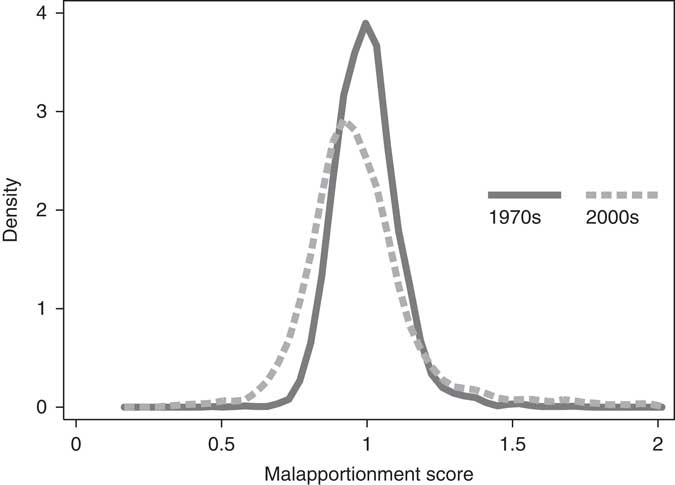
Fig. 1 Malapportionment over time

Since I focus on the effects of malapportionment in India’s state legislatures, I compare the extent of malapportionment across India’s states and over time in Table 1. This indicates, for example, that the largest constituency in Andhra Pradesh in 1978 had a malapportionment score of 1.34, while the smallest constituency had a malapportionment score of 0.74. This means that a citizen’s vote in the smallest constituency was worth approximately double that of a citizen’s vote in the largest constituency. By 2004, a citizen’s vote in Andhra Pradesh’s smallest constituency was worth eight times as much as that of a citizen’s vote in the state’s largest constituency. In the case of the worst offender, Gujarat in 2007, an individual’s vote in the smallest constituency was worth twenty-five times a person’s vote in the largest constituency. Estimates show that states that have experienced rapid economic growth since the 1970s are the ones that were the most malapportioned thirty years later.Footnote ²³ Overall, while a small proportion of state assembly constituencies was 10 per cent smaller or larger than the average constituency size in the late 1970s,Footnote ²⁴ 50 per cent of assembly constituencies fell out of the $\pm$ 10 per cent range of the average constituency size in the 2000s. This table also reconfirms the key assumption of the first mechanism proposed here: malapportionment creates more small than large constituencies. For example, the ratio of constituencies with malapportionment scores $\leq\! $ 0.9 to those with malapportionment scores $\geq\! $ 1.1 is 2:1 in Andhra Pradesh in 2004, and 3:2 in Assam in 2006.

Data and Empirical Strategy

I use repeated cross-sectional data from India’s seventeen largest states (which encompass more than 97 per cent of India’s population; the country has twenty-eight states) from 1977–2007 to test my hypotheses.Footnote ²⁵ The dataset draws on state election dataFootnote ²⁶ and newly collected data on the composition of cabinets for each state approximately one year after every election;Footnote ²⁷ 116 state cabinets were formed during this time. As every state constituency enters the dataset after an election in that state (in other words, observations are for constituency-election years), there are over 23,000 observations. The dataset spans 1977–2007 because constituency boundaries were fixed in that period. Table 2 displays summary statistics for key dependent and independent variables.

A potential problem faced by efforts to estimate the impact of malapportionment is that malapportionment might be endogenous to the outcomes of interest, and the direction of the resulting bias in the estimated effect of malapportionment is ambiguous. For example, if those in power seek to perpetuate their hold on it by creating small districts – as was the case with England’s ‘rotten boroughs’ – the estimated effect of malapportionment will be inflated. If, on the other hand, the powerful create large constituencies because it pays to represent them, estimates of the effects of malapportionment will be attenuated. Save for a few exceptions,Footnote ²⁸ most studies do not address the problem of the endogeneity of malapportionment.Footnote ²⁹

The endogeneity problem might, in principal, be caused by reverse causality, omitted variables and errors in measuring the independent variable. To deal with these issues, I proceed on four fronts. First, I examine the causes of malapportionment in India and rule out the possibility of reverse causality, hypothetical examples of which were listed previously. Secondly, I employ the fullest possible set of constituency and legislature (that is, state-year) fixed effects to control for omitted variables that might cause the error term to be correlated with malapportionment. Constituency fixed effects control for omitted factors at the constituency level that are fixed or only vary slightly over time, including land area, the proportion of minorities (which is largely stable over time) and the like. Since each of the legislature (state-year) fixed effects is a cabinet-formation opportunity, these control for year-invariant, state-invariant and state-year-invariant factors such as patterns of political competition, national and state electoral waves, cabinet size and so forth. They also control for state-level trends, such as levels of economic development. The resulting estimates allow us to recover the effects of changing malapportionment within a constituency and over time, while controlling for factors specific to state-years and those that vary at the state level over time.

Thirdly, I check to see if the results are robust to dropping observations where politicians have the strongest incentives to influence constituency size (for example, those as redistricting approaches), to replacing malapportionment with lagged malapportionment (which is pre-determined but not exogenous), to controlling for malapportionment and lagged malapportionment, and to controlling for the effective number of parties. Lastly, I employ an alternative research design due to the redistricting of 2008 to better control for omitted variables, although this has drawbacks as well. While none of these methods entirely controls for endogeneity, their joint use should help improve inference.

In the rest of this section, I use archival and secondary research to explain why the Congress Party froze reapportionment, and why subsequent governments maintained the freeze.Footnote ³⁰ I consider both the law’s publicly declared goals and aims that may be imputed to it. This analysis largely rules out the possibility of reverse causality in the relationship between malapportionment and cabinet inclusion. As detailed below, the analysis controls for any remaining marginal influence that politicians could have over the size of their constituencies.

The officially declared aim of the freeze in political constituencies in 1976 (which was reiterated in discussions about the partial extension of the freeze in 2003) was to avoid penalizing regions that were effectively curbing their fertility rates. It was thought that regular reapportionment, by reducing the proportion of legislative seats allotted to low-population-growth regions, would blunt these regions’ incentives to implement family planning programs. Surprising as it may seem, it is my contention that the freeze in malapportionment was genuinely instituted and maintained to help fulfill this population control aim.

To see why this is the case, consider the history of the delimitation freeze of 1976. It was part of the infamous forty-second constitutional amendment of India, a fifty-nine-clause piece of legislation that was passed by a chastened Indian Parliament at the behest of Indira Gandhi’s government during the country’s authoritarian interlude. All opposition leaders were in jail during the constitutionally declared ‘emergency’, and a number of opposition parties boycotted parliament. Although the few attending Members of Parliament (MPs) debated the bill over fifteen days, specific clauses were hardly discussed, and almost no amendments were made to the bill. The five clauses of the bill that dealt with the decennial reapportionment process in India were only directly referred to by one MP, who, taking the logic of the measures all too seriously, called for apportionment on the basis of the 1951 census.Footnote ³¹

Several MPs also rose to urge the government to vigorously pursue birth control measures, which the freeze in reapportionment was thought to be a part of. That Sanjay Gandhi, the prime minister’s son, led unlawful forced sterilization drives at the time with impunity illustrates the fixation that people had with population control. Also indicative of this concern were suggestions by MPs to grant women the ‘right’ to deny their husbands more than three children,Footnote ³² the dubbing of large families a crime,Footnote ³³ and the suggestion that politicians with twoFootnote ³⁴ or threeFootnote ³⁵ children should be required to be sterilized if they wish to run for political office. That the freeze in reapportionment was explicitly mentioned as a ‘motivational measure’ in both the 1976 and 2000 national population policies,Footnote ³⁶ which were announced before the 1976 and 2003 constitutional amendment bills were introduced in parliament, also indicates that the government’s intentions were genuine.

Those who dismiss the declared aim of the policy as a foil for something else point to its logical infirmities. They argue, first, that it is doubtful that the freeze would appreciably alter the incentives to curb population growth. Secondly, the modification of the one-man, one-vote principal in the pursuit of one specific policy objective (that is, the reduction in fertility rates) seems suspect. And thirdly, the policy effectively penalizes states (since it leads to their citizens being granted fewer votes in the legislature) that have high population growth rates for reasons (such as improved health and increased economic activity, which lead to a reduction in the death rate and increased in-migration, respectively) other than high fertility. At worst, these criticisms suggest that India’s MPs were foolish. They do not tell us, however, whether policy makers genuinely intended the freeze in malapportionment to help curb population growth rates or not.

There are three other reasons why the reapportionment freeze could have been instituted. First, some have argued that the freeze helps maintain the electoral balance between northern and southern states in India. Southern states, with about one-third of the seats in the Indian Parliament, are the primary beneficiaries of this freeze since their populations have grown less rapidly than those of northern states.Footnote ³⁷ The parliamentary record does not suggest, however, differential support for reapportionment legislation from southern vs. northern politicians. Moreover, simulations suggest that if parliamentary constituencies were reapportioned today, southern states would lose less than 2 per cent of their seats in parliament.Footnote ³⁸ Surely there were other ways for southern states to ensure that their representation was not gradually eroded over time?Footnote ³⁹ And if the only purpose of the freeze in constituencies was to lock in a southern state advantage, why was the redistricting of state assembly constituencies suspended as well? Most importantly, the idea that southern states were trying to lock in an advantage need not concern us here because any such advantage would hold in the national legislature, and not within each of the country’s state legislatures. Since this is a study of the effect of malapportionment on government formation across India’s states, and not in the country’s national legislature, this concern need not detain us further.

Secondly, the Congress Party could have instituted the freeze because it thought it would benefit from it in the future. Yet a close reading of the more than 1,600 pages of parliamentary debates that have occurred over the past thirty years with regard to reapportionment shows that there was not a single accusation of partisan bias leveled against the Congress Party. Accusations of partisan bias also seem unrealistic because the various non-Congress governments that have been in power over the past thirty years did not lift the freeze. Also, malapportionment could only have helped the Congress Party a decade or two along, and it is doubtful that in 1976 the Congress was looking to lock in an advantage that far ahead, particularly given the uncertainty at the time. Further, it is far from clear whether the Congress Party would have had the requisite ability or information to plan that far ahead. That there is no simple relationship between malapportionment and the land area of constituencies, which Figure 2 suggests, supports this argument: if there were such a relationship, legislators could have used land area to predict future malapportionment. Lastly, analysis of the partisan bias that was caused by malapportionment over the past thirty years does not reveal any systematic pro-Congress bias. Table 3 details the partisan bias due to malapportionment, calculated using the methodology proposed by Johnston, Rossiter and Pattie.Footnote ⁴⁰ It shows, for example, that malapportionment secured for the Congress Party an extra 1.4 per cent of seats in Andhra Pradesh in 2004, while it deprived the Bharatiya Janata Party of 4.7 per cent of seats in Karnataka in 2004. This is the first analysis of the partisan effects of malapportionment in India. The table suggests that partisan bias in favor of winning parties, and particularly the Congress Party, was too small and variable for the parties to have wanted to tamper with the reapportionment process, even if they had perfect foresight.

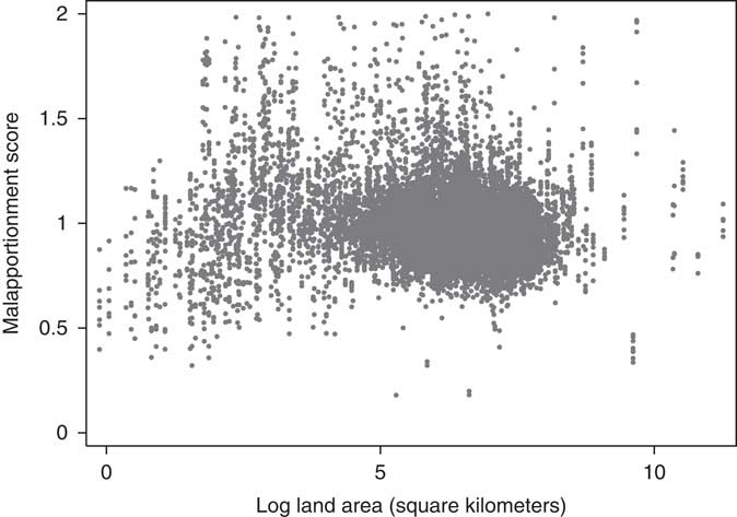
Fig. 2 Malapportionment and land area

Thirdly, it is possible that the freeze in malapportionment was simply instituted by legislators due to ‘a fear of change’.Footnote ⁴¹ While this may be a reasonable rationale for individual legislators to support the freeze in reapportionment once it was proposed, it is not a strong enough reason for Congress Party leaders to have introduced the freeze in the first place since it would, by strengthening individual incumbents, weaken party leaders vis-à-vis legislators. In fact, much of Mrs. Gandhi’s actions at the time were explicitly designed to undercut individual legislators.Footnote ⁴² This rules out a ‘fear of change’ as the reason why the freeze in reapportionment was proposed, although it might help explain why the freeze has been sustained all these years.

To summarize, I have argued that the freeze in reapportionment – which is the deep cause of malapportionment – was genuinely instituted to curb population growth. It was probably sustained thereafter to further this objective, and due to individual legislators’ fear of redrawing boundaries. Given this, the precise degree of malapportionment across state constituencies will depend on differences in birth and death rates, and rates of in- and out-migration between state-level constituencies. Of these two, the first is likely to be the major cause of malapportionment in India, since poverty levels and caste and linguistic fragmentation constrain the movement of people within the country.Footnote ⁴³ Since constituency-level fertility and death rates are not directly manipulable by politicians, I argue that malapportionment is plausibly exogenous to the outcomes that we consider below. That said, and as mentioned, a number of the robustness tests I employ below directly address the possibility that politicians manipulate constituency populations at the margin.

Evidence

Table 4 presents the results of logistic regressions of the effects of malapportionment on cabinet inclusion. The first regression estimates the bivariate relation between the malapportionment score and a dummy for cabinet inclusion, and shows that the two are positively related to one another, which is the opposite of what we would expect. The next regression controls for over 3,500 constituency fixed effects, and thereby estimates the effects of changing malapportionment within constituencies. This regression controls for a variety of unobserved factors that are fixed or only vary slightly over time, including land area, the proportion of minorities, reservationsFootnote ⁴⁴ and so forth. The estimated effect of malapportionment now takes on its expected negative sign. Being from a larger-than-average constituency, ceteris paribus, reduces the chances of a representative being in the cabinet. As the next regression shows, these results remain robust to the inclusion of 115 legislature (that is, state-year) fixed effects. These fixed effects control for cabinet-formation opportunities, and therefore for factors such as patterns of political competition, national and state electoral waves, and cabinet size. They also control for some time-varying factors: specifically, those that vary by state and over time, such as levels of economic development.Footnote ⁴⁵ This is my preferred specification, since it controls for the greatest possible confounds. It indicates that an increase in malapportionment is, as predicted by Hypothesis 1, associated with a decrease in the chances of cabinet inclusion.

It is worth noting that these regressions deliberately do not control for whether legislators are members of the largest party or coalition, since doing so would lead to ‘post-treatment bias’.Footnote ⁴⁶ Malapportionment could indirectly affect cabinet inclusion through its effect on the odds of relatively small constituencies being in the largest party. Indeed, this is what the first mechanism proposed in the theory section argues. This makes controlling for being in the largest party an appropriate way to test for the mechanism by which malapportionment affects cabinet inclusion. I conduct this exercise below, when I consider the mechanisms through which malapportionment has its effects.

The estimated impact of malapportionment on inclusion in the cabinet is large: a one-standard-deviation (0.16) increase in a constituency’s malapportionment score leads to a 2.6-percentage-point fall in the probability that the constituency’s representative is in the cabinet. Given that an average of 12 per cent of legislators are in the cabinet, malapportionment reduces the probability of a legislator being in the cabinet by 22 per cent. This effect is non-trivial, particularly given the considerable agenda-setting, supervisory and spending powers that cabinet members have.Footnote ⁴⁷

The preceding analysis suggests that a citizen from a large constituency faces two distinct, empirically decomposable penalties to his or her representation in the executive due to malapportionment. The first of these is mechanical, and is simply caused by the fact that cabinet members are drawn from a malapportioned legislature. Recall that a citizen’s vote in a constituency with a malapportionment score of 1.16 (that is, in a constituency that is one standard deviation larger than the average constituency) is worth 1/1.16 $\,\approx\,$ 0.86 times the vote of a person in a correctly apportioned constituency. If cabinet members were drawn from the legislature without regard to constituency size, 0.86 would also be the value of this person’s vote in the executive. Secondly, per Hypothesis 1, we know that large-constituency representatives suffer the penalty of not being selected into the cabinet as often as representatives of smaller constituencies. This devalues the vote of a person from a large constituency by a further 22 per cent (this is, per the discussion above, the fall in the probability of a legislator whose constituency has a malapportionment score of 1.16 being selected into the cabinet) to 0.67. In other words, while malapportionment mechanically leads to a person’s vote being worth 0.86 in the legislature, the drawing of cabinets from legislatures further devalues the vote of a citizen from a large constituency to 0.67 in the cabinet.

I conclude this section by considering an observable implication of the account described here. In the period under study, the party system across India’s states underwent a dramatic change, with the median number of parties increasing from 2.1 in 1977 to 3.5 in 2007. This increase in electoral competition was accompanied by a near doubling in median cabinet size from fifteen to twenty-seven ministers, as more parties were accommodated in state cabinets. The fragmentation of the party system should have blunted the effect of malapportionment, as cabinet positions became less scarce. To test this observable implication, I interact malapportionment with a dummy for observations with above-average effective number of parties. The result of this exercise, reported in regression 4 of Table 4, confirms that the effect of malapportionment on cabinet inclusion is indeed somewhat attenuated (although not to a statistically significant degree) as the number of parties increases. This suggests scope conditions for the account proposed in the article: the effects of malapportionment on cabinet inclusion should particularly hold when there are fewer legislative parties and smaller cabinets.