3.1 A brief history of life insurance valuation: multiple reporting measures and valuation approaches

Many life insurance companies produce three forms of published accounts, unusually among industries:

1. 1. returns to regulators, designed to demonstrate the ability of companies to maintain solvency and meet claims to policyholders;

2. 2. statutory accounts under local Generally Accepted Accounting Principles (GAAP), which for many countries has recently been under the International Financial Reporting Standards (IFRS) banner, and

3. 3. embedded values (EVs), produced voluntarily for external publication, internal financial management or both.

Regulatory rules have traditionally differed from region to region. Historically, these rules specified formulaic approaches to valuation (for example, the net premium valuation approach), although more recently discounted cash flow (DCF) techniques have become more common. Assumptions underlying the regulatory valuation have typically been set by an actuary, often with discretion. Assets and liabilities have been measured on either a book or market basis or a hybrid approach.

Primary financial statements have historically been based on local GAAP. For life insurance the local GAAP accounts have often been largely based on the regulatory balance sheets (calculated according to local regulatory rules) with certain adjustments. Assets and liabilities have been measured on either a book or market basis or a hybrid approach.

The origins of EV techniques can be traced back to Anderson (Reference Anderson1959). At a time when regulatory rules specified formulaic approaches to valuation, this paper argued for a valuation and pricing method based on projecting future cash flows using best estimate assumptions and discounting the emerging surpluses using a risk discount rate reflecting the shareholders’ required rate of return and the degree of risk in the blocks of business being valued. EV techniques were therefore an early application of the DCF approach to insurance valuation and were designed to give shareholders more meaningful information than the regulatory or GAAP approaches.

In the 50 years that followed, the main developments in these areas have been:

• – Wide acceptance of the DCF approach as the most realistic measure of reporting for life insurance businesses.

• – The improvement in computer power and construction of complex computer models, allowing companies to value huge portfolios of business using the DCF approach within a relatively short timeframe.

• – The development of analytical tools to determine an analysis of the change in values over time.

• – The widespread use of DCF techniques and EVs by company management to aid in making business decisions, measure performance and as a basis of remuneration.

• – The increasing acceptance of DCF techniques within regulatory reporting and primary accounts.

• – The increasing acceptance of MCV techniques within DCF approaches.

3.2 More MCV within regulatory reporting

In certain countries, companies have recently been required to produce regulatory returns with certain elements valued using market-consistent techniques. For examples, see ASSA (2008), Swiss FOPI (2004) and Swiss FOPI (2006); and for UK with-profits business Hare et al. (Reference Hare, Craske, Crispin, Desai, Dullaway, Earnshaw, Frankland, Jordan, Kerr, Manley, McKenzie, Rae and Saker2004) and Dullaway & Needleman (2004).

For companies in the European Union, the adoption of Solvency II will lead to a market-consistent approach being required for the insurance company balance sheet. Solvency II is led by the European Commission with the objective of improving the protection for policyholders by requiring a more dynamic risk-based approach to setting regulatory reserves and required capital than has been the case under existing Solvency I regulations.

The European Council and Parliament agreed and adopted a final text of the Solvency II Directive dated 10 November 2009, referred to later in this paper as “Solvency II Directive” or European Commission (2009a). The Directive is based on a market-consistent valuation of assets and liabilities.

However, most of the specific requirements within this market-consistent framework will only be agreed as part of the Level 2 implementing measures and Level 3 guidance, where the European Commission is being assisted by CEIOPS and other European bodies such as the CEA, CFO Forum, CRO Forum and Groupe Consultatif. Regulators in countries outside the European Commission are following developments with interest, with some planning to adopt similar measures. Ultimately the European Commission, Council and Parliament are expected to decide on the exact Level 2 implementing measures for Solvency II, during 2010 and 2011. During 2009, the Committee of European Insurance and Occupational Pensions Supervisors (CEIOPS) published a series of consultation papers and “final advice” on various aspects of the Level 2 implementing measures. The European Commission is not bound to accept the recommendations within CEIOPS’ final advice. See European Commission (2009b) for a request for CEIOPS to revisit certain elements of its final advice.

CEIOPS published a final specification for the fifth Quantitative Impact Study (QIS5) in July 2010, broadly consistent with CEIOPS’ final advice in many areas but departing in certain aspects, generally reflecting feedback from the European insurance industry and the European Commission.

3.3 More MCV within primary accounts

Historically, the International Accounting Standards Board (IASB) has, in some areas, been quick to adopt market-consistent valuation techniques within elements of IFRS, although this has generally not been extended to the accounting for insurance contracts. In particular:

• – In 2001, the IASB published a Draft Statement of Principles (IASB, 2001) setting out a set of principles for insurance contract valuation which would in practice require market-consistent valuation techniques. There were, however, a number of restrictions in the application compared to an approach more closely aligned with economic value, for example the treatment of renewal premiums and market value margins, Dullaway & Foroughi (Reference Dullaway and Foroughi2002).

• – the IASB then published a series of IFRSs (IASB, 2004-5) which were adopted by members of the European Union and many other countries. IAS 39 defines the classification and measurement of financial instruments. IFRS 4 governs the accounting for insurance contracts but was designed as an interim standard, allowing grandfathering of existing local GAAP approaches for the measurement of insurance contract liabilities, subject to a number of minimum standards. A market-consistent approach was permitted within IFRS 4 but not encouraged or required, Lloyds TSB (2006) describes how Scottish Widows’ embedded value was restated on to a market-consistent EEV basis and for the “insurance business” carried into the primary accounts under IFRS 4.

• – The IASB published the Discussion Paper “Preliminary Views on Insurance Contracts” on 3 May 2007, setting out a building block approach for measuring the insurance contract technical provision underpinned by market-consistent valuation techniques. However there were a number of important differences compared to a more realistic approach; see Dullaway et al. (Reference Dullaway, Foroughi and Wright2007) for a description.

The IASB's Insurance Contracts project has since become a joint project with the United States’ Financial Accounting Standards Board (FASB).

The IASB published its exposure draft on the Insurance Contracts project on 30 July 2010 (IASB, 2010), requesting comments from the insurance industry by 30 November 2010. The final insurance contracts standard is expected to be published by the summer of 2011.

The IASB exposure draft broadly follows the IASB (2007) approach to construct an insurance contract measurement model using a market-consistent building block approach, stating in paragraph IN13:

1. (a) a current estimate of the future cash flows

2. (b) a discount rate that adjusts those cash flows for the time value of money

3. (c) an explicit risk adjustment

4. (d) a residual margin…”

Paragraph 17 defines the residual margin as an amount that

This decision on the residual margin leads to restrictions placed on the timing of profit recognition and so moves the valuation model away from an economic value approach.

The IASB exposure draft describes differences with the FASB approach. One main difference is the desire of the FASB to combine the explicit risk adjustment and the residual margin building blocks.

3.4 More MCV within embedded values

The use of MCV techniques has perhaps been most widespread in recent years among companies publishing embedded values, where the term market-consistent embedded value (MCEV) has become commonly accepted. The first MCEVs were published by AMP (2003) and Royal & Sun Alliance (2003).

This was closely followed by the CFO Forum publishing the European Embedded Value Principles (“EEV Principles”) in May 2004, which set out an external financial reporting framework with extensive disclosure requirements. The EEV Principles permitted, but did not require, a market-consistent approach to be used to set the overall allowance for risk. The use of the market-consistent approach within EEV was advocated by True et al. (Reference True, Taylor-Gooby, Whitlock, Byrne, Hoffmann, Milton, Jones, Hales, Kalberer and Melody2004), Dullaway & Whitlock (Reference Dullaway and Whitlock2005) and O’ Keeffe et al. (Reference O’ Keeffe, Desai, Foroughi, Hibbett, Maxwell, Sharp, Taverner, Ward and Willis2005).

The first companies adopting the EEV Principles at year-end 2004 generally adopted a “top-down” approach to allow for risk in the risk discount rate, similar to that advocated in Anderson (Reference Anderson1959) and historical traditional embedded value (TEV) practice. Companies adopting in later years tended to use the MCV approach to allow for risk. This trend is shown in Table 1. Up to year-end 2007 there was broad consistency but some differences in approaches used under the “MCV banner” (Foroughi et al., Reference Foroughi, Alargé Salvans, Bause, Cartier, Creedon, Gose, Hugmark, Harewood, Kapel, Lebel, Milton, Mirani and Whitlock2008a). This led to calls in the industry for the CFO Forum to prescribe and standardise an MCV approach within the EEV Principles.

Table 1 Approaches to allow for risk within EEV/MCEV Principles publications, year-end 2004–2009

Source: Aaron et al. (Reference Aaron, Bause, Buck, Cartier, Creedon, Escudero, Foroughi, Gose, Guiry, Harrison, Hugmark, Milton, Pater and Vandenbosch2010).

On 4 June 2008, the CFO Forum published the original MCEV PrinciplesFootnote 1, (Copyright Stichting CFO Forum Foundation 2008), which prescribed a market-consistent approach to the allowance for risk within embedded values. Upon publication, all members of the CFO Forum pledged a compulsory adoption of the MCEV Principles from year-end 2009. This CFO Forum publication is summarised in Coughlan et al. (Reference Coughlan, Demerle, McGuffie, Paton, Purves and Sanner2008a) and Foroughi et al. (Reference Foroughi, Alargé Salvans, Bause, Cartier, Creedon, Gose, Hugmark, Harewood, Kapel, Lebel, Milton, Mirani and Whitlock2008b).

The evolution of companies adopting market-consistent valuation techniques to allow for risk within published embedded values under either the EEV Principles or MCEV Principles is shown in Table 1.

The financial crisis, in particular following Lehman Brothers’ collapse in September 2008, led to a number of MCV technical decisions being revisited. The CFO Forum announced on 19 December 2008 that:

At year-end 2008, following the onset of the recent financial crisis a proliferation of “MCV” approaches arose under ‘market-consistent’ EEV Principles or the MCEV Principles (with areas of material non-compliance), described in detail in Foroughi et al. (Reference Foroughi, Alargé Salvans, Bause, Cartier, Creedon, Gose, Hugmark, Harewood, Kapel, Lebel, Milton, Mirani and Whitlock2009a).

Consequently, in an announcement dated 22 May 2009, the date for compulsory adoption of the MCEV Principles was postponed from 2009 to 2011. The June 2008 MCEV Principles were revised on 20 October 2009 (CFO Forum, 2009), with the main revision being the potential inclusion of a liquidity premium above the swap yield curve. The October 2009 MCEV Principles are summarised in Foroughi et al. (Reference Foroughi, Alargé Salvans, Bause, Cartier, Creedon, Gose, Hugmark, Harewood, Kapel, Lebel, Milton, Mirani and Whitlock2009b).

4.1 The “market-consistent valuation” concept

The “market-consistent valuation” concept aims to ensure that the allowance for risk within a valuation is calibrated to market prices of risk where relevant and reliable.

In a market-consistent valuation framework, assets and liabilities are valued in line with market prices and so consistently with each other. In principle, each projected cash flow is valued in line with the prices of similar cash flows that are traded on the open market. For example, the cash flows arising from an equity are valued in line with the market price of the equity, the cash flows from a bond in line with the price of that bond, and so on. Furthermore, liability cash flows (which are not usually traded) are valued in line with the traded assets they most closely resemble. A fixed liability due in ten years would be valued in line with a 10-year zero coupon bond and an embedded financial option in line with the market price of a similar option.

In practice, a number of short cuts and alternative approaches (for example certainty equivalent valuation and risk-neutral stochastic valuation) are used. These make the valuation process easier whilst achieving the objective set out in the preceding paragraph.

The market-consistent valuation concept and the description and application of these short cuts are described in more detail in Dullaway (Reference Dullaway2001), Dullaway & Foroughi (Reference Dullaway and Foroughi2002), Blight, Kapel & Bice (Reference Blight, Kapel and Bice2003), Exley & Smith (Reference Exley and Smith2003), Foroughi et al. (Reference Foroughi, Jones and Dardis2003), Tillinghast (2003), Sheldon & Smith (Reference Sheldon and Smith2004), Dullaway & Whitlock (Reference Dullaway and Whitlock2005), O’ Keeffe et al. (Reference O’ Keeffe, Desai, Foroughi, Hibbett, Maxwell, Sharp, Taverner, Ward and Willis2005), CFO Forum (2008, 2009), IAA (2009), Foroughi (2009) and Varnell (Reference Varnell2009).

4.2 The case for MCV

As well as having to satisfy external demands for MCV information, companies have increasingly used MCV techniques in setting ALM and investment strategies, monitoring performance against planned activities, negotiating M&A transaction prices and pricing new business.

Reasons for these developments include the following:

• – It offers decision makers the ability to meaningfully compare the relative value of alternative courses of action.

• – The allowance for risk within the MCV approach is more objective than under alternative approaches, creating greater confidence in the results among stakeholders.

• – The allowance for risk is more granular, giving more meaningful information about segmental results.

• – It is easier to achieve consistency between the asset and liability valuation, helping to ensure that variances in the profit and loss account/analysis of movement result from asset liability mismatches and not accounting mismatches.

• – By valuing liabilities with reference to the market price of a closely matching asset, the MCV information is of relevance from a solvency perspective and helps a company make Asset Liability Management (ALM) and risk management decisions.

• – The MCV analysis of movement, variances and sensitivities give an insight into the sources of value creation and can feed into the business control cycle decision-making process and risk management. (See Section 6 for a further description of the analysis of movement and sensitivities.)

5.1 Some MCV commercial challenges

Recent MCV developments have led to a number of commercial challenges:

1. 1. An MCV measure may lead to much greater volatility of balance sheet and earnings than non-MCV measures.

In principle, the MCV approach should lead to volatility arising due to real asset liability mismatches, not accounting mismatches. Therefore, the MCV approach should exhibit lower volatility if assets and liabilities are well matched.

1. 2. It is not clear how to price new business in markets where other market participants base prices on non-MCV measures.

Where other market participants base prices on non-MCV measures, particularly where expected investment spreads are allowed for in the valuation, companies face a strategic challenge in deciding whether to follow such prices (potentially writing the new business at an MCV loss) or reduce market share.

In the short term, a company may wish to continue selling in the market to maintain its franchise value, particularly if it believes that it will be able to achieve expected investment spreads and other metrics (such as those set out in Section 6) support the new business strategy.

However in the long run, a company may wish to consider whether to raise prices. One point of view is that there is a disconnect if policyholders are receiving the benefit of expected investment spreads (via the pricing of the business), whereas shareholders are bearing the risk associated with achieving these spreads, and yet are not being compensated for taking this risk. A harder pricing market may result.

1. 3. In extreme financial conditions, the MCV approach can lead to a procyclical effect on the values of financial assets, potentially leading to adverse effects on otherwise sound insurance companies and industries.

This is addressed in section 15.

1. 4. The points above can discourage insurance companies from investing more in credit risky assets that are otherwise a good match for the liabilities, leading to knock on macroeconomic effects such as higher prices for policyholders and reduced availability of credit.

This is not specifically addressed further in this paper.

1. 5. The MCV does not provide information on the capital requirements and capital generation characteristics of the business.

This is addressed in section 6.

5.2 Addressing these challenges – an overview of the rest of this paper

The rest of this paper addresses these MCV challenges as follows:

• – Section 6 describes a recommended financial reporting information pack.

• – Sections 7 to 14 describe the technical challenges underlying the MCV calculation and recommend some enhancements in light of the recent financial crisis. Some of these dampen the procyclicality effect.

• – Section 15 describes the procyclical effect in more detail recognising it as an important political concern, and describes some methods which can be applied in mitigation.

• – Section 16 then provides a final thought on the subject of MCV.

6.2. Analysis of movement of MCV

The analysis of movement in market-consistent valuations during a reporting period is a useful tool to indicate the performance of a block of business or company. One such approach is that mandated for companies publishing under the MCEV Principles and is reproduced in Table 2 below. This approach originates from insurance company practice and a rationale is set out in Collins & Keeler (Reference Collins and Keeler1993).

Table 2 Movement analysis (Source: CFO Forum MCEV Principles Appendix A)

⁽¹⁾This represents the following two components:

▪ Expected earnings on free surplus and required capital; and

▪ Expected change in VIF

⁽²⁾The earnings assuming assets earn the beginning of period reference rate

⁽³⁾The earnings is the component in excess of the reference rate reflecting the additional return consistent with the expectation of management for the business.

The analysis is on a net of taxation basis with movements disclosed on a line-by-line basis.

The MCEV Principles provide a glossary of terms used in this table (including the MCEV components free surplus, required capital and VIF) and guidance in calculating and allocating sources of surplus to the various elements of the analysis.

This analysis is useful in managing business from a number of perspectives:

• – The analysis of MCEV movement is often used as a measure of performance and as a basis of remuneration.

• – Different areas of the business can take responsibility for the business performance shown in different elements of the analysis.

• – The separate identification of the value of new business within this analysis, including a product breakdown, provides a useful input into decisions on new business pricing and product strategies.

• – A split of this analysis into the relevant components of MCEV (free surplus, required capital and value of in force) helps to assess any implications for dividend paying capacity. In particular, the capital generation of in-force business can be compared with the capital strain of writing new business. This helps address point 5 in section 5.1 above.

• – The analysis of variances broken down by source of risk is useful information for those responsible for setting best estimate assumptions.

6.3 MCV sensitivities

The sensitivity of the market-consistent value to risks helps in risk management, risk quantification and in highlighting the materiality of specific assumptions.

The MCEV Principles mandate publication of economic and non-economic sensitivities.

Economic sensitivities include change in the interest rate environment, change in equity/property capital values, changes in equity/property implied volatilities and changes in swaption implied volatilities.

Non-economic sensitivities include changes in maintenance expenses, lapse rates, mortality and morbidity rates.

The MCEV Principles mandate specific quantums of sensitivities. Users are often interested in other quantums as well.

The MCEV Principles generally mandate pessimistic economic scenario sensitivities. Users are often interested in optimistic economic scenario sensitivities as well, particularly in times of financial crisis.

Additional sensitivities not mandated by the MCEV Principles but which are of interest to users of the information include:

• – a credit spread sensitivity (which affects the assumed market value of corporate bonds and other credit-risky assets, with consequential impact on those liabilities affected by credit risk).

• – a liquidity premium sensitivity (see Section 10 for a description of the liquidity premium).

Interestingly, a number of European-headquartered companies are providing MCEV sensitivities within the primary accounts under the section on risk disclosures (as required by IFRS 7 Financial Instruments: Disclosures), using the supplementary embedded value reporting calculations instead of, or in addition to, the sensitivities of the IFRS equity.

6.4 Primary account and regulatory account information

While primary and regulatory balance sheets are constructed in a different manner to the market-consistent approach, companies have to calculate these balance sheets as well, and users will be interested in the results.

Insurance companies will then face a challenge in communicating the differences in balance sheets and earnings analysis between the various reporting metrics, particularly as these explanations are likely to involve the differences in the technical aspects of the underlying calculations.

This challenge is discussed in more depth in Foroughi (Reference Foroughi2010b), with Table 3 proposed as a possible solution. The article includes a detailed explanation of the rationale, structure and contents of the table. The main elements are as follows:

Table 3 A proposed analysis/reconciliation of earnings across reporting measures

• – The analysis follows a similar structure to the MCEV Principles Appendix A.

• – The possible asset adjustments incorporate the revaluation to fair value of those financial instrument assets not measured at fair value in the primary accounts.

• – The liability adjustments include setting the residual margin to nil for insurance contracts, and revaluing those contracts classified as “investment contracts.

• – “Economic equity” is a realistic measure of MCV.

• – The Solvency Capital is the Solvency Capital Requirement under Solvency II.

• – The Free Surplus is defined such that the Solvency Capital and Free Surplus is the available capital under Solvency II, adjusted to allow for any margins within the Solvency II valuation of assets and liabilities other than Technical Provisions.

• – The Value of In Force is the margins within the Technical Provisions measurement.

6.5. Analysis of the movement in the levels of assets

For savings products where the earnings by the insurer are related to the levels of assets, users of the information are interested in an analysis of the movement in the levels of assets, indicating how much the levels of assets have moved over a period due to for example new business sales, investment performance and decrements such as lapses. Such analysis is also referred to as “analysis of net fund flows”.

6.6 Projected “real world” distributable earnings

Users of the information are also interested in projected distributable earnings calculated on a “real world” economic best estimate basis, i.e. including expected asset risk premia. This information helps the user assess the expected timing of return of capital, as well as providing information on the expected reward for the company given the risks taken on.

DCF applications in TEV and other industries are often calculated on a similar basis as well. This information helps to relate the valuation of a block of insurance business with information available in other industries. A number of metrics can be calculated from the projected real world distributable earning (and underlying cash flow projections), described below.

6.7 Implied risk discount rates

Once projected real world cash flows are calculated, implied risk discount rates (“IDRs”) can be calculated showing what aggregate discount rate should be used to convert the projected real world cash flows into the market-consistent value at the valuation date. IDRs are therefore a measure of the theoretical minimum required return to capital providers given the risks inherent in a block of business.

6.8 New business information

Clear and complete new business information can help provide users of the information with insights into the new business strategy and the capital that is being used to write new business. In addition to market-consistent new business values (identified within Table 2), useful information includes:

7.2 Current exit value or fulfilment value

Practitioners are faced with two general approaches to the calibration of the allowance for risk:

• – a “current exit value”, that is the value a third party would pay to purchase an asset or the consideration required for a third party to accept a liability obligation, also known as transfer value.

• – a “fulfilment value”, that is the “in-use”Footnote 2 market value of the asset or the cost to the insurer of fulfilling the obligation, sometimes referred to as going concern value or settlement value.

The Solvency II Directive contains elements of a current exit value approach to valuation. Article 75 (1) of the final text of the Solvency II Directive states “assets shall be valued at the amount for which they could be exchanged between knowledgeable willing parties in an arm's length transaction” and separately states “liabilities shall be valued at the amount for which they could be transferred, or settled, between knowledgeable willing parties in an arm's length transaction”.

IASB (2007) puts forward a current exit value approach to setting insurance contract liabilities, stating:

Interestingly, IASB (2010) makes no overall mention of a current exit value concept, instead stating in paragraph 17

However, paragraph 35 of IASB (2010) describes the risk adjustment as

This appears to introduce some aspects of a current exit value, albeit based on the insurer's own perspective rather than that of a market participant.

No focus is given to a current exit value by the EEV and MCEV Principles when calibrating the allowance for risk. Principle 3 of both publications states the

The practical difficulty with the current exit value concept is that it does not reflect how insurers generally manage their business. Transfers of business between one insurer and another do not happen frequently and hence no reliable market price exists for calibration. In addition, transfers generally occur due to merger and acquisition activity, and are usually on the basis that one insurer transfers a block of business containing both assets and liabilities to another insurer. The consideration paid in respect of the transfer of the assets and liabilities often depends on many qualitative factors influencing both buyer and seller.

The MCEV Principles recognise these complications when stating “the allowance for risk should be calibrated to match the market price for risk where reliably observable.” In addition G.3.3 states “the concept of mark to market is to value insurance liabilities and therefore the shareholders’ interest in the earnings distributable from assets allocated to the covered business as if they are traded assets with equivalent cash flows. However, most insurance liabilities are not traded. As assets are generally traded with an observable market price, asset cash flows that most closely resemble the insurance cash flows (from the shareholders’ perspective) are used.”

Interestingly the IAIS also recognises that the concept of a “current exit value” is somewhat theoretical and is, in practice, related to the fulfilment concept. IAIS (2007) states “the IAIS believe that any transfer notion would be strongly influenced by the settlement [fulfilment] obligations that the transferee would undertake”.

I recommend the fulfilment value approach to calibrating the allowance for risk.

Practitioners that have to perform a current exit value allowance for risk calibration (for example to follow prescribed rules) should also pay close regard to the fulfilment value approach in order to avoid the potential for an unreliable calibration.

7.3 Consistency in the overall allowance for risk

When considering the overall allowance for risk, it is important to ensure consistency between the valuation of assets and liabilities. Consistency is easier to achieve if the allowance for risk is considered across both assets and liabilities together.

The developments within Solvency II, IASB and FASB (see quotes in section 7.2 above) mean that assets and liabilities are calibrated and valued separately, increasing the risk of inconsistency in the overall calibration.

In contrast, the EEV and MCEV Principles’ philosophy of calibrating the allowance for risk to blocks of business (containing both assets and liabilities) helps to ensure consistency in the overall valuation.

This concept of consistency influences a number of recommendations made in later sections.

7.4 Clarity over areas of judgement

The remainder of this paper illustrates the challenges with calibrating a robust MCV at times of financial crisis. Calibration is often much easier in more benign financial market conditions.

I recommend ensuring the disclosure accompanying MCV makes clear the extent to which judgement is required. An approach set out in FAS 157 Fair Value Measurement (FASB, 2006) and followed in recent IFRS disclosure requirements is to require a Three Level Hierarchy:

Level 1: unadjusted quoted prices in active markets for identical assets or liabilities that the reporting entity has the ability to access at the measurement date.

Level 2: Inputs other than quoted prices included within Level 1 that are observable for the asset or liability, either directly or indirectly. Examples include quoted prices for similar assets or liabilities in active markets.

Level 3: unobservable inputs for the asset or liability.

Disclosure regarding the fair value of assets under each level of hierarchy can help the reader assess the areas of judgement with financial instrument valuation.

Similar information can be provided for the valuation of insurance liabilities, by considering the equivalent calibration asset. A number of companies publishing market-consistent EEVs or MCEVs have provided some related information in the disclosures, for example indicating where extrapolation is required and the materiality on the result.

8.1 Background and recent developments

Historically, the MCV approach sets the valuation of financial instruments to market value. However the recent financial crisis has led to much greater illiquidity in a number of asset classes with subsequent concerns about the reliability of quoted market prices. This has led to the question of how to assess whether markets are “deep and liquid” and the related question of what is the market-consistent value of illiquid assets.

Recent developments in this area have been led by both the FASB and the IASB.

In April 2009, the US accounting regulator FASB published Staff Position Paper FAS 157-4 (FASB, 2009) addressing how to determine fair value in illiquid markets.

The IASB announced in April 2009 a comprehensive and urgent review of both IAS 39 Financial Instruments: Recognition and Measurement, and the more general concept of “fair value”.

The IAS 39 review led to the publication of IASB (2009b), then to the publication of the financial asset classification and measurement standard IFRS 9 (IASB, 2009c) which comes into effect in 2013 with early adoption permitted. IFRS 9 requires companies to classify and measure financial assets as either “amortised cost” or “fair value”, with the company's business model and the characteristics of the asset influencing the classification. IFRS 9 does not yet cover the impairment model for assets measured at amortised cost and hedge accounting and in these areas the IAS 39 review is ongoing.

The IASB's Fair Value Measurement Exposure Draft (IASB, 2009a) proposes that the core principle of the fair value of assets is to determine “the price that would be received to sell an asset … in an orderly transaction between market participants at the measurement date”.

Both FAS 157-4 and IASB (2009a) recommend using a mark-to-model approach when markets are no longer orderly. The aim of such a mark-to-model approach is to estimate what the market price would be in an orderly market, taking into account all available information.

These publications provide guidance in what constitutes a disorderly market, much of which relates to the depth and liquidity of the market. Examples are set out in IASB (2009a) Appendix B5 and are extracted below:

1. (a) there has been a significant decrease in the volume and level of activity for the asset or liability when compared with normal market activity for the asset or liability (or similar assets or liabilities).

2. (b) there are few recent transactions.

3. (c) price quotations are not based on current information.

4. (d) price quotations vary substantially over time or among market-makers (eg some brokered markets).

5. (e) indices that previously were highly correlated with the fair values of the asset or liability are demonstrably uncorrelated with recent indications of fair value for that asset or liability.

6. (f) there is a significant increase in implied liquidity risk premiums, yields or performance indicators (such as delinquency rates or loss severities) for observed transactions or quoted prices when compared with the entity's estimate of expected cash flows, considering all available market data about credit and other non-performance risk for the asset or liability.

7. (g) there is a wide bid-ask spread or significant increase in the bid-ask spread.

8. (h) there is a significant decline or absence of a market for new issues (ie primary market) for the asset or liability (or similar assets or liabilities).

9. (i) little information is released publicly (eg a principal-to-principal market).

10. (j) An entity evaluates the significance and relevance of the factors (together with other pertinent factors) to determine whether, on the basis of the evidence available, a market is not active.”

A similar list can be found in FAS 157-4.

When valuing financial instrument assets within markets judged to be orderly, IASB (2009a) requires companies to use observed market prices.

When valuing financial instrument assets where that asset's market price is not observable, IASB (2009a) requires companies to use a mark-to-model approach.

Judgement is required for financial instruments where market prices are observable, but the presence of a number of the other conditions described above suggest disorderly markets. An illustrative example may be the corporate bond markets in late 2008, where observed yields rose significantly over a short time period. However, companies found that volumes of trades fell significantly over the same period, with both buyers and sellers unable to transact meaningful sized trades at observed market prices. The implementation of IASB (2009a) would require companies in such circumstances to judge whether the fair value core principle would lead to a different price than the observed market price.

However, a fair value standard has not yet been published and is not expected to come into effect until around 2012.

The Solvency II QIS5 specification makes no explicit reference to this type of situation when describing the valuation of the assets. There is a general reference to IASB fair value but no further consideration or discussion about how to determine fair value in inactive markets or consider whether markets are active or inactive.

In the context of valuing the technical provisions, QIS5 specification TP.2.98. states:

In this context, QIS5 specification TP.4.4. goes on to define the required financial market conditions as follows:

1. “(a) a large number of assets can be transacted without significantly affecting the price of the financial instruments used in the replications (deep),

2. (b) assets can be easily bought and sold without causing a significant movement in the price (liquid),

3. (c) current trade and price information are normally readily available to the public, in particular to the undertakings (transparent).”

8.2 Valuation of financial instrument asset recommendations

9.1 Background

The reference rate is the yield curve used, in a market-consistent valuation framework, to discount cash flows which are not affected by investment market movements. It is also the yield curve used to project and discount cash flows which vary linearly with investment market movements (the “certainty equivalent” approach) and the yield curve used within stochastic models designed to determine a market-consistent value of embedded financial options and guarantees.

This section focuses on items to consider when selecting the reference rate with the exception of the liquidity premium. Section 10 discusses items to consider when deciding whether to also apply a liquidity premium, and if so how to calibrate the liquidity premium. It is noted that the phrase “reference rate” is generally defined to include any liquidity premium included in its calibration.

For a number of years up to end 2007, companies using the market-consistent approach within regulatory returns, primary accounts or embedded values tended to use a government bond or swap based calibration of the reference rate, with no additional adjustment. However, at year-end 2008 many companies departed from this practice.

Reasons provided for changes in the calibration of reference rates included reference to the illiquidity premium of assets and/or liabilities, and the higher yields on government bonds relative to swaps.

Table 4 summarises practice among CFO Forum companies at year-end 2008 in this area. Similar inconsistency can be observed in some companies’ year-end 2008 IFRS and regulatory disclosures.

Table 4 Reference rates within year-end 2008 ‘market-consistent’ EEV or MCEV Principles publications

Source: Foroughi et al. (Reference Foroughi, Alargé Salvans, Bause, Cartier, Creedon, Gose, Hugmark, Harewood, Kapel, Lebel, Milton, Mirani and Whitlock2009a).

A similar table found in Aaron et al. (Reference Aaron, Bause, Buck, Cartier, Creedon, Escudero, Foroughi, Gose, Guiry, Harrison, Hugmark, Milton, Pater and Vandenbosch2010) shows that practice became more standardised at year-end 2009. This may have been driven more by reductions in liquidity premia observed in the market from year-end 2008 to year-end 2009 than increased standardisation of practice in setting the reference rate.

CEIOPS (2009a, 2009c) sets out and describes a number of criteria used to assess possible reference rate calibrations, including: no credit risk, realism, reliability, highly liquid for all maturities, no technical biases, available for all relevant currencies, and proportionate.

CEIOPS (2009a, 2009c) generally proposed a AAA government bond based calibration, and rules out the use of swap yield curves given the perceived credit risk inherent within these instruments. However, this is one of the tentative decisions that European Commission (2009b) recommended be revisited, and it is noted that in many currencies for periods from year-end 2008 swap yields at medium to longer durations are lower than equivalent government bond yields (see Figure 1).

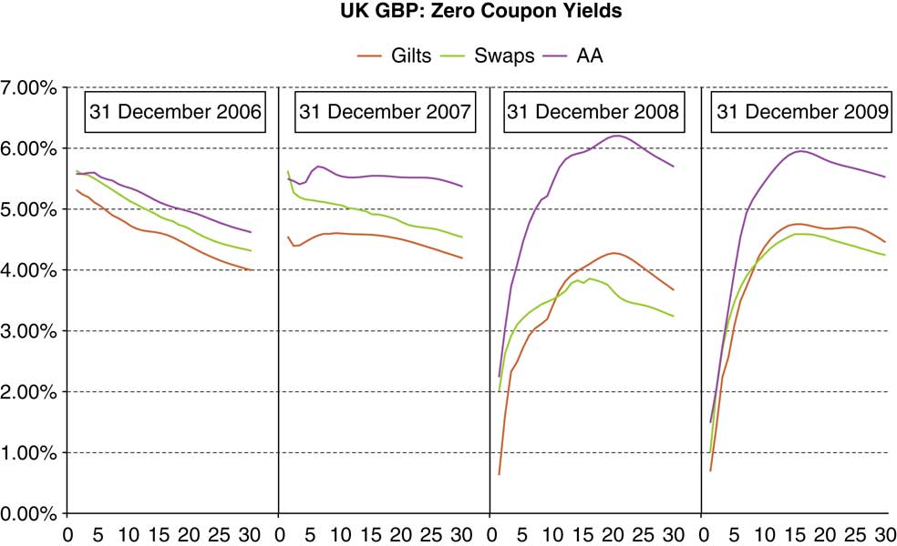
Figure 1 Government bond, swap and AA corporate debt spot yields, 2006–2009

Source: Towers Watson analysis of Bloomberg data

CFO Forum (2008, 2009) requires a swap based calibration where swap yields are available, although CFO Forum (2009) permits an adjustment to swap rates to allow for a liquidity premium under certain circumstances.

For QIS5 (2010) reference rates are provided for standard currencies. They are based on swap yields (where these are available), with a 10 bps reduction to allow for the perceived level of credit risk in the swap yield and a liquidity premium addition which varies by the nature of the liabilities (details provided in section 10).

Neither CEIOPS (2009a, 2009c), nor QIS5 (2010), nor CFO Forum (2008, 2009) advocate an upwards adjustment to the calibration asset to allow for additional own credit risk.

IASB (2007) describes the following in calibrating the reference rate:

IASB (2010) describes the following in calibrating the reference rate (referred to in the exposure draft as the “discount rate”), in paragraphs 30 and 31:

1. (a) are consistent with observable current market prices for instruments with cash flows whose characteristics reflect those of the insurance contract liability, in terms of, for example, timing, currency and liquidity.

2. (b) exclude any factors that influence the observed rates but are not relevant to the insurance contract liability (eg risks not present in the liability but present in the instrument for which the market prices are observed).

Paragraph 34 of IASB (2010) covering the liquidity premium is quoted in ¶10.2.3.

9.2 Recommendations

I recommend that reference rates (before considering the liquidity premium) are calibrated using similar principles to CEIOPS (2009a, 2009c) except for the following:

9.3 Comparison of recent government bond and swap yield curves

When assessing the ‘minimum cost’ valuation premise, it is useful to note that the relationship between government bond and swap yields can vary quickly over time. Figure 1 compares government bond, swap and AA corporate debt spot yields, within the UK at year-end 2006, year-end 2007, year-end 2008 and year-end 2009.

Some observations from Figure 1:

• – AA corporate bond yields widened significantly compared to both gilts and swaps from year-end 2006 to year-end 2007 and from year-end 2007 to year-end 2008. Although AA corporate bond spreads have narrowed during 2009, this may in part be due to downgrades within the corporate bond sector.

• – Swap spreads (over UK government bonds or gilts) were around 20–40bp at most durations at 31 December 2006.

• – At 31 December 2007, swap spreads had widened to 80-100bp at durations 1 and 2 and 30–60bp at most other durations.

• – At 31 December 2008, the feature of negative swap spreads was apparent, with a crossover between 10 and 11 years. At most long durations swap spreads were lower than gilts by around 30–70 bp.

• – At 31 December 2009 the crossover point had shortened to between 8 and 9 years. However negative swap spreads reduced compared to 31 December 2008. At most long durations swap rates were lower than gilts by around 10–30bp.

There are a number of possible explanations for the recent development of negative swap spreads at medium to long durations:

• – swap contracts offer a rolling credit check on the security of the counterparty, a feature not found within government bond contracts.

• – government bonds require purchase with 100% cash, whereas swap contracts can be purchased with margin and hence there is a much smaller initial cash outlay. Swaps may therefore be more attractive at medium to long durations.

• – the supply of government bonds has increased since the onset of the recent financial crisis in many markets, and this is expected to continue for several years; although in certain markets this may be offset by quantitative easing policies.

• – arbitrageurs are less active than in the period prior to the recent financial crisis, and hence are less likely to interact between the government bond and swap markets to take advantage of negative swap spreads.

In my opinion these reasons add to the advantages of applying the ‘minimum cost’ valuation premise set out in Section 9.2.2.

10.2 Liquidity premium developments within Solvency II and Phase II

There have been two significant liquidity premium developments within Solvency II during 2010, set out below.

10.2.1 March 2010 CIEOPS-led Illiquidity Premium Taskforce report

On 17 November 2009, CEIOPS was asked by the European Commission to set up a task force to develop technical solutions to the illiquidity premium, as well as the potential use of swaps as the base risk free rate, and the method for the extrapolation of the yield curve at long durations. In addition to CEIOPS members, the task force included representatives from the Groupe Consultatif, CFO Forum, CRO Forum, CEA, AMICE and the European Commission.

On 3 March 2010, the CEIOPS-led task force published its report concentrating on the potential use of an illiquidity premium in Solvency II, and also covering the choice of risk-free rate and extrapolation. This was accompanied by a cover letter from CEIOPS to the European Commission.

The aspects of the report concentrating on the illiquidity premium are summarised in Towers Watson (2010) as follows:

“The report recommends the following, if an illiquidity premium is to be used:

The report recognises the possibility that in future some illiquidity premium adjustment may be made to the Solvency II valuation of assets, reflecting possible FASB/IASB fair value accounting developments. The phrase “consistent with solvency valuation methods” in principle 6 avoids the risk of double counting.

10.2.2 European Commission (2010) QIS5 specification

The QIS5 specification published in July 2010 allows a liquidity premium with certain conditions. The full liquidity premium is defined for each standard currency at 31 December 2009 using the methodology described in the CRO Forum/CFO Forum calibration paper on the risk free interest rates, which was based on long term illiquid financial assets maturing in that currency.

The QIS5 specification (when published in draft form in April 2010) was accompanied by a CFO Forum/CRO Forum calibration paper entitled “QIS5 Technical Specification Risk-free interest rates”. That paper sets out the following formula, which was originally set out in the task force report, to calculate the liquidity premium for major currencies:

The “Spread” used above is based on corporate bond indices relative to swaps.

For non-standard currencies, no liquidity premium can be used if it is not possible to follow the CRO Forum/ CFO Forum methodology in a robust manner (e.g. due to the lack of appropriate or adequate long-termed illiquid assets, or lack of reliable prices or data, or the principles aforementioned on the illiquidity premium are not met).

QIS5 requires a proportion of this full liquidity premium to be added as an adjustment to the reference rate depending on the nature of the liabilities, following Principle 4 of CEIOPS (2010). The proportion does not depend on the assets held, following Principle 2 of CEIOPS (2010).

The QIS5 specification has taken a “bucket” approach to differentiate between liabilities where the full liquidity premium is allowed and those where a lower allowance is appropriate. Under QIS5 only liabilities that meet the following criteria get the full 100% liquidity premium allowance. The appropriate bucket is defined for an insurance contract, with all the cash flows of a contract receiving the same allowance:

1. 1. the only underwriting risks connected to the contracts are longevity risk and expense risk;

2. 2. the undertaking does not bear any risk in case of any form of surrender

3. 3. the premiums have already been paid and no incoming cash-flows are allowed for in the technical provisions of the contracts.

With profits contracts other than those with the 100% allowance should be discounted with a 75% liquidity premium allowance. All other contracts should use 50% allowance.

10.3. What is meant by ‘liquidity premium’ in an MCV context? Two perspectives

The term ‘liquidity premium’ is often used in the context of market-consistent valuations, but there is no one clear definition.

The idea that more liquid assets have a higher price than less liquid assets as a consequence of being more easily tradeable is well established, and the impact of liquidity on asset prices has been observed during the recent financial crisis. However, this implies that one of the market risk premia required within assets is an “asset illiquidity risk premium”. This in itself does not enable a liquidity premium to be allowed for in the MCV of an insurance block of business, consisting of both assets and liabilities.

One interpretation of the term “liquidity premium” in an MCV context is to measure an insurance liability as an equivalent hypothetical asset which produces broadly similar cash flows, with similar levels of liquidity or illiquidity to the liability. This is implied by IASB (2010) paragraph 34 quoted above, and appears to be the direction of Solvency II QIS5.

However, this interpretation ignores the point of view that the term “liquidity” in this context relates to assets, not liabilities. Liabilities are generally by nature illiquid, as in most circumstances the liability holder does not have the right to force the asset holder to trade.

My preferred interpretation of the term “liquidity premium” in an MCV context is a related but different term. This term is described in Byrne & Dullaway (Reference Byrne and Dullaway2009), Dullaway (Reference Dullaway2009) and Foroughi et al. (Reference Foroughi2009a, b), as an asset liability management context which combines both asset illiquidity and the associated spreads with liability predictability and stability. The existence of predictable and stable liability cash flows enables an insurance company to match those cash flows with an illiquid but otherwise low risk asset, as their need for asset liquidity is likely to be less than that for the average market participant. With this interpretation, the availability of illiquid assets to match the liabilities becomes more important.

10.4 Question when calibrating the MCV liquidity premium

I believe the following is a critical consideration when calibrating the MCV liquidity premium:

Should the MCV liquidity premium for a particular block of business be restricted to the asset illiquidity risk premium that canbe derived from viable ALM investment strategies available to the insurance company in managing the block of business?

I believe that in order to ensure consistency in the valuation between assets and liabilities, and to ensure a link between the MCV model and ALM strategies, the answer to the above question should be “Yes”.

Reasons I think practitioners should answer “Yes” to this question include the following:

• – this recognises that the features of markets which typically lead to a material asset illiquidity risk premium, namely that they are not perfectly efficient and can at times be extremely inefficient (for example late 2008 and early 2009), are the same features that inhibit insurers who do not already own illiquid assets from taking advantage of the MCV liquidity premium. A lack of restriction would therefore lead to the risk of using too much liquidity premium in the valuation, introducing an accounting mismatch.

• – demonstrating the ability to capture asset illiquidity risk premium is important information to management and other stakeholders, and should give more credence to the MCV liquidity premium assumption used.

However, other parties appear to be heading towards a different conclusion. For example:

• – while the CEIOPS (2010) advocates in its liquidity premium principle 3 “the extra return which can be earned by the insurer holding illiquid assets free of credit risk”, there is no mention of the potential restriction from this principle in the QIS5 specification. The liquidity premium calibration in QIS5 is derived solely from the liquidity premium formula set out in section ¶10.2.2 and the features of the liabilities.

• – IASB (2007) and IASB (2010) do not consider the above question or the potential implications resulting from a “Yes” response.

• – Pritchard & Turnbull (Reference Pritchard and Turnbull2009) describe the liquidity premium in a liability only context, containing a useful analysis of restrictions that may arise on being able to capitalise the liquidity premium as a result of unpredictability and instability of liability cash flows. However, one of the central tenets of Pritchard & Turnbull (Reference Pritchard and Turnbull2009) is that an MCV consists of a market value of assets less a transfer value (current exit value) of liabilities (consistent with the Solvency II Directive), and that this results in the liquidity premium calibration being independent of an insurer's own investment strategy (whether actual or achievable). Section 7 of this paper sets out why this is not my preferred interpretation of an MCV.

10.5 Measures to assess asset illiquidity risk premia

A number of measures are available to assess the asset illiquidity risk premiaFootnote 3, including:

• – monitoring the residual spreads available from corporate bond yields less the cost of credit default swaps compared with a measure of the reference rate (typically swaps)

• – using structural asset models such as the model described in Merton (Reference Merton1974) to decompose corporate bond spreads into credit yields and the remainder (including illiquidity). A recent example of applying this approach can be found in Webber & Churm (Reference Webber and Churm2007)

• – monitoring yields in other asset classes such as collateralised or covered bonds.

• – I believe it is useful to compare the results of multiple methods when assessing the liquidity premium, as the various methods have their own strengths and weaknesses.

However, where the objective is to measure the liquidity premium within the corporate bond market and residual spreads are reliably available, my preference is the residual spread approach for the following reasons:

• – it represents a direct market-calibrated measure of the residual spread available in corporate bonds, a natural upper boundFootnote 4 for the liquidity premium. By way of contrast, results from the structural asset model approach may reflect imperfections in the structural asset model. Results from the covered/collateralised bond approach may reflect market perceptions about the covered/collateralised bond market (noting that the collateral often consists of banks’ mortgage assets) rather than liquidity available in the corporate bond market.

• – subject to certain conditions, a corporate bond less a credit default swap can be considered a viable calibration asset for a predictable liability cash flow and so can be considered in the context of the ‘minimum cost’ valuation premise described in section 9.2.2.

• – at times of financial crisis insurance companies holding corporate bonds can (with certain limitations which are at times significant) purchase credit default swaps to provide credit protection, instead of selling the corporate bonds. The existence of the credit default swap market can therefore better enable insurance companies to capture the liquidity premium within ALM strategies. This additional risk management tool should be of interest to other stakeholders as well.

10.6 Observable residual spreads

Figure 2 highlights residual spreads calculated from the Eurozone and US dollar corporate bond and credit default swap indices, during the period January 2007 to December 2009, as well as how these residual spreads compare with sample levels from the QIS5 calibration. (Calculating these residual spreads is not straightforward.)

Figure 2 Eurozone/US dollar average residual spreads over swaps (2007–2009; average up to 10 years) and QIS5 liquidity premium relative to swaps

Sources: Towers Watson analysis of Bloomberg and Markit data; QIS5 technical specification including data from accompanying paper CFO Forum/CRO Forum (2010)

Some observations from Figure 2:

• – residual spreads were very low (under 20bp) from January 2007 to the onset of the credit crunch in August 2007, and fairly low (under 50bp) for many periods from August 2007 to August 2008. Similar levels of spreads can be found earlier in the 2000s.

• – this suggests the swap yield curve was a good proxy for a reference rate for several years prior to September 2008.

• – residual spreads significantly increased during September 2008 and remained high until April 2009.

• – residual spreads fell significantly from the September 2008-April 2009 peak to year-end 2009.

For currencies other than Eurozone and US dollars, my understanding is that credit default swap indices are not currently available, so the residual spread approach requires calculation using individual corporate bond and credit default swap prices. This process is much more challenging for practitioners.

10.7 Recommendations

In terms of measuring the level of asset illiquidity risk premia, CEIOPS ( 2010) and CFO Forum/CRO Forum ( 2010) provide a helpful starting point with the proposed formula (reproduced above). Such a simplified method is to be welcomed as it enables the industry to move on from how much illiquidity is found within asset yields, to how much should be capitalised in a market-consistent valuation. A comparison of the formula with residual spreads suggests a broadly consistent calibration; however there is a case for increasing the assumed level of liquidity premium particularly at times of financial crisis. One mechanism to achieve such a result would be to increase the “50%” factor, possibly mitigated by an increase in the “40bp” factor to reduce the effect in more benign times.

In terms of recommended restrictions, a number are set out in more depth in Footnote 5. Considerations which I believe are important but which do not seem to appear in either the Solvency II QIS5 specification or the IASB Insurance Contracts Exposure Draft are as follows:

1. (i) Companies should consider whether the liquidity premium could be captured in practice, via investment in asset classes with observable illiquidity risk premia. Approaches include considering the current ALM investment strategy and viable ALM investment strategies which could be implemented at reasonably short notice.

2. (ii) Given that many illiquid assets also contain material levels of credit risk, when considering how much liquidity premium can be captured in practice, one should take into account the potential inability of an insurer to decouple credit risk from illiquidity risk in many assets and consequential restrictions on the investment strategy.

3. (iii) If the liquidity premium calibration assumes a hypothetical investment policy with a much greater proportion in illiquid assets than the existing investment policy, the depth and liquidity of the calibration asset markets used should be considered. This helps an insurer assess whether the liquidity premium calibration represents a viable investment strategy.

4. (iv) Liquidity premia are usually measured against observed market prices. If the valuation of assets assumes a mark-to-model approach which leads to a fair value higher than observed market prices, then the upper bound liquidity premium (asset illiquidity risk premium) should be reduced accordingly.

11.1. Background: Own credit risk and the measurement of liabilities

The global financial crisis has made the role of credit risk in liability measurement more prominent. During late 2008, asset values fell as market and credit risk premia increased. Liability values also fell if their measurement included an allowance for own credit risk. This was particularly the case for the valuation of corporate debt and pension scheme liabilities, where the use of a corporate bond based discount rate led to falls in the values of liabilities.

In principle, there is nothing to stop a limited allowance for own credit risk to be made within an MCV, reflecting the limited ability of an insurance company to default on its policyholder provisions. Indeed, the calibration of the reference rate to swaps in the June 2008 MCEV Principles was accompanied by a recognition that swaps contain some credit risk. However, given the protection to policyholders arising from the insurance regulatory regime, and the typical higher ranking of policyholder debt over other creditors on wind up, it would be expected that policyholder debt has much stronger credit protection than corporate debt issued by the same company.

An upper bound for the measure of own credit risk may be found in the credit default swap market, although this should be reduced for:

• – the higher ranking of policyholder debt.

• – the level of credit risk in the calibration instrument(s) used to determine the reference rate and liquidity premium, to avoid double counting.

Whether or not an MCV should allow for own credit risk within the liability valuation is debatable. The IASB's June 2009 Credit Risk in Liability Measurement Discussion Paper sets out a more general analysis of the advantages and disadvantages of allowing for own credit risk in accounts, and O’ Keefe et al. (Reference O’ Keeffe, Desai, Foroughi, Hibbett, Maxwell, Sharp, Taverner, Ward and Willis2005) Appendix B sets out some advantages and disadvantages in an MCEV context.

Interestingly the FASB and IASB appear to rule out an insurer-specific and up-to-date explicit allowance for own credit risk in the valuation of insurance liabilities with Phase II, stating in IASB (2010):

The Solvency II Directive states in Article 75 “When valuing liabilities under point (b), no adjustment to take account of the own credit risk standing of the insurance or reinsurance undertaking shall be made.” This applies not only to insurance liabilities, but to all liabilities, including corporate debt or pension scheme obligations. A strict interpretation of this phrase may lead to no own credit risk being allowable for such liabilities, which would lead to a prudent regulatory balance sheet. What is not clear is the interpretation of the phrase “no adjustment”, and it is to be hoped that clarity will be provided as part of Level 2 Implementing Measures.

The QIS5 specifications have added an extra word to the Directive phrase in the context of valuing financial (not insurance) liabilities, stating “no subsequent adjustment to take account of the change in own credit standing of the insurance or reinsurance undertaking should be made.” This appears to change or clarify the meaning of this phrase, and may explain the QIS5 approach to valuing corporate debt as set out in Section 14.

At times of financial crisis, own credit risk may be an important element in the overall valuation of an insurance company, depending on the purpose of the valuation. In extreme market conditions, companies can and do fail, for example insurance companies in Japan in the late 1990s and early 2000s as described in Freeman & Fujiki (Reference Freeman and Fujiki2001).

11.2 Recommended approach

For MCVs calculated on a fulfilment value approach, I recommend that no additional allowance for insurance liability own credit risk be made in an MCV beyond that implicit in the reference rate and liquidity premium calibration, primarily for the following reasons:

• – It is easier to buy back debt or renegotiate pension scheme promises than negotiate to not meet policyholder promises, suggesting that greater levels of “own credit risk” may be present in these liabilities than insurance liabilities. (The valuation of non-insurance liabilities in discussed in Section 14.)

• – The franchise value of insurance companies is generally made up of the value associated with selling future new insurance business, and this would likely be impacted in a scenario where existing policyholder promises are not met.

If an additional allowance is made, the assumption and impact on value should be disclosed separately.

I recognise that some implicit own credit risk will exist in the MCV as a result of the recommendations set out in Section 9.2, namely that government bond or swap yields are not adjusted to remove credit risk embedded in the instrument and the ‘minimum cost’ valuation premise is applied to permit the higher yielding instrument. The allowance for liquidity premium described in Section 10 may (depending on the calibration) also increase the level of implicit own credit risk.

Notwithstanding this recommendation, there are specific circumstances where an additional allowance for own credit risk within the MCV should be considered. These include:

• – industries where regulators permit the insurance company to renegotiate policyholder debt in specific extreme circumstances without triggering bankruptcy (strictly this may therefore not be a credit default event but is a risk of non-performance by the insurer).

• – when calculating MCV for internal purposes, depending on the purpose own credit risk may be considered in the context of risk appetite and risk management. Stakeholders may wish to consider under what circumstances insurance companies may default on their obligations.

12.1 Implied volatilities – recent practice

For a number of years up to end 2007, companies that published EEVs using the market-consistent approach calibrated the stochastic models for valuing embedded financial options and guarantees to either a government bond-based or swap yield curve (typically a swap yield) and to valuation date implied volatilities.

However, at end 2008 many companies departed from this practice. Table 5 summarises practice among CFO Forum companies (for source see Foroughi et al., Reference Foroughi, Alargé Salvans, Bause, Cartier, Creedon, Gose, Hugmark, Harewood, Kapel, Lebel, Milton, Mirani and Whitlock2009a).

Table 5 Implied equity option and swaption volatilities within year-end 2008 ‘market-consistent’ EEV or MCEV Principles publications

1. Disclosed that end November was used for practical reasons and that this was similar to an end December calibration.

Reasons provided within the relevant publications for not using valuation date implied volatilities included a lack of deep and liquid options markets, unusual characteristics in the options markets, dislocated financial markets and a practical inability to calibrate to higher volatilities.

Practice within market-consistent primary accounts and regulatory returns was less clear.

Interestingly, by end 2009 (Aaron et al., Reference Aaron, Bause, Buck, Cartier, Creedon, Escudero, Foroughi, Gose, Guiry, Harrison, Hugmark, Milton, Pater and Vandenbosch2010) show how these companies had all returned to calibrating the implied equity option and swaption volatilities to end December 2009. These companies generally did not indicate whether this change of methodology was driven by changes in the views of the depth and liquidity of options markets or changes in the levels of option prices.

12.2 Stochastic model calibration – key consideration

The following is a key consideration when calibrating the stochastic model used to value embedded options and guarantees:

In an MCV, is it desirable for the stochastic model to reproduce the market prices of relevant traded options with features most similar to those of the liabilities?

Provided it is accepted that reproducing market prices of relevant traded options is a desirable feature, then practitioners have a choice when calibrating the stochastic model:

• – observed implied volatilities can be used only if standard Black Scholes (equity) or Black's Formula (fixed interest) models are used and the reference rate used is the swap yield curve. This reflects the standard practice among investment market traders in quoting implied volatilities.

• – if a different stochastic model or reference rate is used, then the implied volatility set in the stochastic model may need to be different from observed implied volatilities to ensure the market prices of traded options are reproduced in the model.

Some practitioners argue that there is too much credit risk in the traded options market and that this credit risk should be removed by replacing the swap yield curve (underpinning implied volatility quotes) with the government bond yield curveFootnote 6.

12.3 Recommendations

12.4 Justifying valuation adjustments in blocks of business with material embedded financial options and guarantees

The recommendations set out in section 12.3 may appear to imply that the main way of valuing a block of business with embedded financial optionality is to use a swap yield curve with no MCV liquidity premium and valuation date-calibrated implied volatilities. (Alternatively, adjustments can be made to both the reference rate and the implied volatility to ensure market prices are reproduced.)

This ignores two credible rationales for making adjustments:

12.4.1 Allowance for a liquidity premium in valuing blocks of business with material embedded financial options and guarantees

The discussion relating to setting the reference rate in section 9 and permitting a liquidity premium in section 10 was in the context of valuing non-option business.

When valuing business with material embedded financial options and guarantees, it is possible to consider the business as comprising a sub-block of business without embedded financial options, and the remainder sub-block which contains the embedded financial options.

This perspective is perhaps easiest when considering the business from a “call option plus cash” perspective, rather than a “put option plus share” perspective. This perspective is set out in more depth in a with-profits fund context in Dullaway & Needleman (Reference Dullaway and Needleman2004) and originates from put-call parity.

At times of material illiquidity in asset markets, it is possible that an insurer would be able to hold illiquid assets to match predictable and stable cash flows and hence may be able to earn substantial illiquidity risk premiums without incurring the extra risk. These illiquid assets are represented in Figure 3 by “cash”.

Figure 3 Put-call parity

The question then is whether an insurance company can justify the use of a liquidity premium in the valuation of the sub-block without embedded financial options, given the restrictions set out in Section 10. These restrictions may be more onerous for such business. For example, the ability to capture liquidity premium may be limited if there are restrictions on the investment strategy of the block of business in question. This is often the case with participating business.

The restrictions may lead to a much smaller liquidity premium adjustment being reasonable for an overall block of business with material embedded financial options and guarantees, as the liquidity premium would only be applicable for the proportion of the business in the sub-block without financial options, and the estimation of such an adjustment is not straightforward.

One caveat is to ensure under such an approach that the stochastic model valuing the option is calibrated to call option implied volatilities, not put option implied volatilities. Call option implied volatilities may be higher if, as a result of the application of the above liquidity premium argument, call options become more popular in the market than put options.

As far as I am aware, no insurance company or standard setter has published this perspective as a rationale for reducing the MCV liabilities from that which would arise using a swap yield curve with no liquidity premium adjustment and implied market volatilities. It would be a challenging explanation to provide to an external user.

13.2 Recommendations

I recommend the following with respect to non-hedgeable risk:

• – An NHR process is followed to identify which non-hedgeable risks are not fully allowed for elsewhere in the valuation and therefore require some additional allowance.

• – the NHR risk margin is set taking into account the elements identified in the above process and also a small charge for uncertainty.

• – clear disclosures are included with the MCV to explain the outcomes of the above and the purpose of any additional allowance for non-hedgeable risk.

To avoid doubt, I envisage the charge for uncertainty being much smaller than the recommendations found in CEIOPS (2009b, 2009c). The rationale is set out below.

A recommended six step NHR process is set out in Figure 4and described in Foroughi et al. (Reference Foroughi, Alargé Salvans, Bause, Cartier, Creedon, Gose, Hugmark, Harewood, Kapel, Lebel, Milton, Mirani and Whitlock2008b). Although this process is designed to demonstrate compliance with the MCEV Principles, I believe that its application fits well with the recommendations found elsewhere in this paper and encourages good risk management.

Figure 4 A recommended six step process to allow for NHR within MCVs

14.1 The valuation of deferred taxation assets and liabilities

The Solvency II QIS5 specification states “The carry forward of unused tax credits and the carry forward of unused tax losses shall be calculated in conformity with international accounting standards as endorsed by the EC”, directing the reader to the relevant international accounting standard IAS 12 Income Taxes.

However there are two non-market-consistent aspects of IAS 12 when it comes to valuing deferred tax assets and liabilities:

• – no discounting is permitted

• – a deferred tax asset or liability should be set up if the future cash flow is “probable” to arise i.e. greater than 50% probability.

I recommend that deferred taxation assets and liabilities are valued using a consistent approach to the rest of the valuation, in particular including the effect of discounting and excluding any restriction if the future cash flow is deemed not “probable” to arise.

I recommend that tax asymmetries should be considered in the overall valuation, either directly in the valuation of deferred taxation assets and liabilities or elsewhere for example the allowance for non-hedgeable risk.

14.2 The valuation of corporate debt liabilities

IAS 39 currently permits companies to value corporate debt liabilities at either amortised cost or fair value, and both practices are widespread in current insurance company accounts.

The CFO Forum 2009 MCEV Principles follow the original EEV Principles in generally requiring in the guidance that corporate debt liabilities are valued at fair value. However, a number of companies that value debt at amortised cost in the IFRS follow that practice in their EEV or MCEV publications, disclosing this aspect of non-compliance with the EEV or MCEV Principles’ guidance.

The Solvency II QIS5 specification states:

I interpret this to mean that QIS5 debt is valued at neither amortised cost nor fair value after day 1, instead it is valued using the level of credit risk inherent in the instrument's value upon initial recognition, and the level of the risk-free rate at the valuation date. It is not clear to me whether in the last sentence of the above quote the term “risk free rate” excludes or includes a liquidity premium, and if the latter the level of liquidity premium to be assumed.

I recommend that corporate debt liabilities are valued at fair value to ensure consistency with the rest of the valuation, and so include the effect of own credit risk in the market value without adjustment.

15.1 Description of procyclicality

There is a macroeconomic risk that a market-consistent reporting framework can lead to procyclicality. Market values fall at times of financial crisis, which can threaten insurers’ solvency. In order to protect solvency, insurers may therefore sell higher risk assets to fund the purchases of lower risk assets. This may in itself lead to further market value falls, again further threatening solvency.

To date, most regulatory regimes have contained discretion in the solvency calculations, and there are a number of elements within regulatory regimes which contain counter-cyclical elements in the methodology and assumptions. With the onset of Solvency II, this discretion and counter-cyclicality may reduce.

15.2. Recognition within Solvency II

It is noted that the Solvency II Directive recognises this risk. Paragraph (16) page 9 of the Directive states “The main objective of insurance and reinsurance regulation and supervision is the adequate protection of policy holders and beneficiaries. The term beneficiary is intended to cover any natural or legal person who is entitled to a right under an insurance contract. Financial stability and fair and stable markets are other objectives of insurance and reinsurance regulation and supervision which should also be taken into account but should not undermine the main objective.”

The Commission has identified that transitional provisions are necessary in the case of discount rates to ensure a smooth transition to Solvency II and avoid temporary market disruption. QIS5 will test the impact on the basis that Solvency II is fully implemented and also what the position would be with the benefit of grandfathering.

15.3 Possible mitigating measures

Some possible mitigating measures are set out below. Specific recommendations are not provided in this paper.

1. Stakeholders (including regulators) should base decisions on multiple metrics and not just a market-consistent valuation framework, and should use judgement in assessing the relevance of each metric to the decisions being made.

This is similar to the background leading to the recommendation in this paper that companies develop a financial reporting pack as set out in Section 6. Different metrics can provide different insights into business performance.

2. Stakeholders should recognise that theories such as the efficient market hypothesis do not hold, particularly at times of financial crisis, and hence enable some flexibility in the valuation of assets and liabilities.

The highest-and-best-use asset valuation premise, the ‘minimum cost’ liability valuation premise and the MCV liquidity premium and allowing a certain level of own credit risk, as described earlier in this paper, are examples where observed inefficiencies in the market are taken into account in the valuation, forming a counter-cyclical effect.

3. The regulatory framework should enable flexibility in the capital requirements (i.e. capital required to be held in addition to that required to meet market-consistent liabilities) at times of financial crisis, to ensure that enforced regulatory or management actions recognise the potential short-term nature of the financial crisis.

4. On the other hand, the onus is on stakeholders to ensure capital requirements in benign financial times are sufficient to absorb losses during financial crises, taking into account levels of asset liability mismatch risk.