


Introduction
Globally, current knowledge of species biology is heavily biased towards the Northern Hemisphere where research infrastructures have been developed over a longer time period (Meyer et al. Reference Meyer, Kreft, Guralnick and Jetz2015). In contrast, taxa inhabiting economically developing countries in tropical regions in the Southern Hemisphere often receive less attention even though these are generally the most biodiverse regions of the world (Wilson et al. Reference Wilson, Auerbach, Sam, Magini, Moss, Langhans, Budiharta, Terzano and Meijaard2016). In particular, species distributional range limits in the Global South are often unknown or little studied, especially for raptors (Buechley et al. Reference Buechley, Santangeli, Girardello, Neate‐Clegg, Oleyar, McClure and Şekercioğlu2019). To address distribution knowledge gaps, Species Distribution Models (SDMs) have become a widely used spatial tool to infer species-habitat associations and identify environmental range limits (Elith and Leathwick Reference Elith, Leathwick, Moilanen, Wilson and Possingham2009, Matthiopoulos et al. Reference Matthiopoulos, Fieberg and Aarts2020). SDMs are statistical methods that correlate the underlying environmental conditions from known species occurrences and predict where similar environmental conditions should exist for a given species (Scott et al. Reference Scott, Heglund, Morrison, Haufler, Raphael, Wall and Samson2002, Pearce and Boyce Reference Pearce and Boyce2006). SDMs are particularly useful for predicting distributions for rare species inhabiting landscapes logistically and physically difficult to survey and thus to estimate range size (Rhoden et al. Reference Rhoden, Peterman and Taylor2017, Sutton and Puschendorf Reference Sutton and Puschendorf2020, Sutton et al. Reference Sutton, Anderson, Franco, M.Clure, M.randa, Vargas, Vargas González and Puschendorf2021a,Reference Sutton, Anderson, Franco, McClure, Miranda, Vargas, Vargas González and Puschendorfb).
The global spatial bias in mapping species distributions is most apparent for species with cosmopolitan ranges spanning both hemispheres. The Peregrine Falcon Falco peregrinus (hereafter ‘Peregrine’), is a widespread raptor with a global range, present on all continents except Antarctica (White et al. Reference White, Cade and Enderson2013). Currently, 18-20 geographical subspecies are recognised (White et al. Reference White, Cade and Enderson2013), with the distribution and habitat requirements of many Northern Hemisphere Peregrine subspecies in Europe and North America well documented (Ratcliffe Reference Ratcliffe1993). The Madagascar Peregrine Falcon F. p. radama (hereafter ‘Madagascar Peregrine’) is one of the least known Peregrine subspecies in terms of biology and distribution (White et al. Reference White, Cade and Enderson2013; but see Razafimanjato et al. Reference Razafimanjato, de Roland, Rabearivony and Thorstrom2007). The subspecies is an uncommon resident with a patchy distribution across upland and coastal areas of Madagascar, Mayotte, and the Comoros Islands (Langrand Reference Langrand1990, Goodman et al. Reference Goodman, Pidgeon, Hawkins and Schulenberg1997, Razafimanjato et al. Reference Razafimanjato, de Roland, Rabearivony and Thorstrom2007).
Nearly all the current literature on the Madagascar Peregrine states the scarcity of the subspecies and logistical difficulties in locating individuals or breeding pairs (reviewed in White et al. Reference White, Cade and Enderson2013). Indeed, the first confirmed nest was only reported in 1983 on the high central plateau near Antsirabe (Langrand Reference Langrand1990). Most reports state that Peregrines are most frequent in the mountainous interior of Madagascar or around rocky seacoasts and islets (Goodman et al. Reference Goodman, Pidgeon, Hawkins and Schulenberg1997, Razafimanjato et al. Reference Razafimanjato, de Roland, Rabearivony and Thorstrom2007), following their general reliance on cliff nesting because the Falconiformes have not evolved nest building (Ratcliffe Reference Ratcliffe1993). Breeding usually starts around mid-May, with juveniles dispersing from their natal areas by the end of November (Razafimanjato et al. Reference Razafimanjato, de Roland, Rabearivony and Thorstrom2007). Madagascar Peregrine diet largely consists of small passerines, such as the widespread Madagascar Bulbul Hypsipetes madagascariensis and Madagascar Red Fody Foudia madagascariensis, though larger prey items such as Columbids (e.g. Madagascar Green Pigeon Treron australis) are also taken (Razafimanjato et al. Reference Razafimanjato, de Roland, Rabearivony and Thorstrom2007).
Due to the limited transport infrastructure to survey remote areas in many regions of Madagascar, assessing distribution status for this subspecies is problematic and logistically challenging (Razafimanjato et al. Reference Razafimanjato, de Roland, Rabearivony and Thorstrom2007). For those species that exist in remote, hard to survey areas, SDMs are effective for estimating distribution using environmental covariates combined with biodiversity inventory occurrence data from sources such as museums, atlases, and community science projects (Bradter et al. Reference Bradter, Mair, Jönsson, Knape, Singer and Snäll2018, Sutton et al. 2021a,b). Despite issues of sampling bias in opportunistically collected inventory data (Newbold Reference Newbold2010), such data often cover a large sampling extent beyond that possible from systemically sampling across large scales. Thus, with improved modelling methods able to account for inherent spatial sampling biases, such as penalized logistic regression models (Phillips et al. Reference Phillips, Anderson, Dudík, Schapire and Blair2017), biodiversity inventory data can help fill knowledge gaps on distribution, habitat extent, and population size.
Defining the habitat extent and range limits of a given species is often the first step in setting conservation planning priorities (Elith and Leathwick Reference Elith, Leathwick, Moilanen, Wilson and Possingham2009). However, standard mapping methods set out by the IUCN (Brooks et al. Reference Brooks, Pimm, Akçakaya, Buchanan, Butchart, Foden, Hilton-Taylor, Hoffmann, Jenkins, Joppa and Li2019) are unable to account for the areas where the focal species may exist but there are few or no occurrence records. Using predictive spatial models can account for these disparities, providing further detail beyond what the standard IUCN metrics can provide (Breiner et al. Reference Breiner, Guisan, Nobis and Bergamini2017, Herkt et al. Reference Herkt, Skidmore and Fahr2017, Sutton et al. 2021a,b). Here, we fit a resource selection function in environmental space using an Ecological Niche Factor Analysis (ENFA) and a Species Distribution Model (SDM) in geographic space using penalized logistic regression in a generalized SDM framework. We thus follow the general analytical paradigm of predicting species range limits based on species-habitat associations (Matthiopoulos et al. Reference Matthiopoulos, Fieberg and Aarts2020). Specifically, our aims are to establish baseline measures of key biological parameters, addressing three significant knowledge gaps for the Madagascar Peregrine: (1) provide the first detailed distribution map and area of habitat, (2) define habitat requirements across the current known range, and (3) calculate a first estimate of population size based on inferred habitat area.
Methods
Study Area
Madagascar, Mayotte, and the Comoros are situated in the tropical zone approximately 400 km from the south-east African mainland in the Indian Ocean. Madagascar is a continental island separated from the African mainland by the Mozambique Channel, with Mayotte and the Comoros a small archipelago of volcanic islands lying 200 km off north-west Madagascar in the northern Mozambique Channel (Figure 1). Madagascar has a highly heterogeneous landscape with an extensive upland plateau running longitudinally along the centre of the island, descending to a wide lowland dry forest coastal plain in the west, an arid region in the south-west, and a narrower coastal strip of humid tropical forest running along the eastern seaboard. Due to this varied landscape and topography, climate is dominated by the north-south central plateau, dictating temperature and rainfall regimes in multiple bioclimatic regions (Jolly et al. Reference Jolly, Oberlé and Albignac2016). Both Mayotte and the Comoros have similar environmental heterogeneity, albeit at a smaller scale, with upland areas, coastal plains, and rocky coasts.
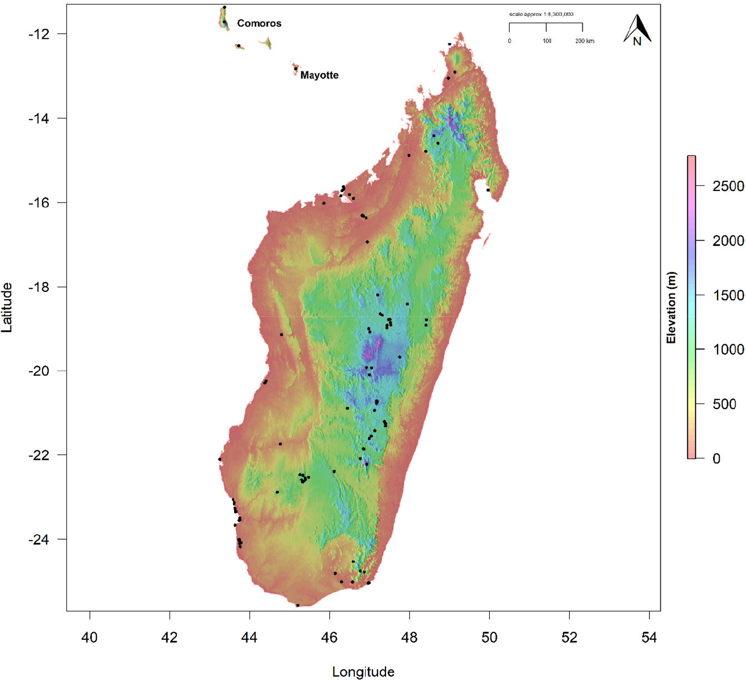
Figure 1. Digital Elevation Model (DEM) for Madagascar, Mayotte, and the Comoros, showing altitudinal range within the current known distribution of the Madagascar Peregrine Falcon. Black points denote Peregrine occurrences.
Occurrences
We sourced Madagascar Peregrine occurrences from the Global Raptor Impact Network (GRIN) information system (McClure et al. Reference McClure, Anderson, Buij, Dunn, Henderson, McCabe and Tavares2021). For the Madagascar Peregrine, GRIN consists of occurrences from the African Raptor DataBank (Davies et al. Reference Davies, Virani, Ogada, Botha, Buij, Brouwer, Barlow, Azafzaf, Kendall, Monadjem, McClure, Rayner, Wroblewski, Trice, Sutton, Baker and Baker2020), eBird (Sullivan et al. Reference Sullivan, Wood, Iliff, Bonney, Fink and Kelling2009), GBIF (2019a,b) and from surveys conducted by Peregrine Fund biologists. We cleaned occurrence data by removing duplicate records, those with no georeferenced location, and any locations over water, resulting in 194 occurrences to use in the calibration models. Only occurrences recorded from 1990 onwards were used to match the timeframe of the environmental data, whilst retaining sufficient sample size for modelling (van Proosdij et al. Reference van Proosdij, Sosef, Wieringa and Raes2016). We reduced sampling bias and clustering in the occurrence points, by applying a 1-km spatial filter between the raw occurrences to minimise the effects of over-sampling in highly surveyed areas (Aiello-Lammens et al. Reference Aiello‐Lammens, Boria, Radosavljevic, Vilela and Anderson2015). We selected the 1-km thinning distance to match the resolution of the environmental raster layers and to capture the high environmental heterogeneity of the study area.
Habitat covariates
We predicted occurrence using habitat covariates representing climate, landcover, topography, and vegetation heterogeneity downloaded from the EarthEnv (www.earthenv.org) and ENVIREM (Title and Bemmels Reference Title and Bemmels2018) repositories. We used a total of six continuous covariates (Table 1) at a spatial resolution of 30 arc-seconds (~1 km resolution), cropped to a delimited polygon consisting of all three range countries. We selected covariates a prioiri based on climate, landcover and topographic variables related empirically to Peregrine distribution (Ratcliffe Reference Ratcliffe1993, White et al. Reference White, Cade and Enderson2013). Heterogeneity is a biophysical similarity measure closely related to vegetation species richness (i.e. vegetation structure, composition, and diversity) derived from textural features of Enhanced Vegetation Index (EVI) between adjacent pixels; sourced from the Moderate Resolution Imaging Spectroradiometer (MODIS, https://modis.gsfc.nasa.gov/). We inverted the raster cell values in the original EarthEnv variable ‘Homogeneity’ (Tuanmu and Jetz Reference Tuanmu and Jetz2015) to represent the spatial variability and arrangement of vegetation species richness on a continuous scale which varies between zero (minimum heterogeneity, low species richness) and one (maximum heterogeneity, high species richness).
Table 1. Habitat covariates used in all spatial analyses for the Madagascar Peregrine Falcon.

The three measures of percentage landcover (Cultivated, Mosaic forest, Herbaceous vegetation) are consensus products integrating GlobCover (v2.2), MODIS land-cover product (v051), GLC2000 (v1.1) and DISCover (v2) from the years 1992–2006. Mosaic forest is derived from the EarthEnv variable ‘Mixed trees’ and represents a mixed landcover of mixed forest, shrubland, and woody savanna. Herbaceous vegetation defines both open and closed grassland cover, with cultivated representing a mix of cropland, tree cover and managed vegetation. Full details on methodology and image processing can be found in Tuanmu and Jetz (Reference Tuanmu and Jetz2014). Elevation was derived from a digital elevation model (DEM) product from the 250m Global Multi-Resolution Terrain Elevation Data 2010 (GMTED2010; Danielson and Gesch Reference Danielson and Gesch2011). Aridity Index is based on the degree of water deficit below a given need (Thornthwaite Reference Thornthwaite1948). The index ranges from zero (low aridity) to one (high aridity). All selected covariates showed low collinearity and thus all six were included as predictors in model calibration (Variance Inflation Factor <2; Table S1 in the online supplementary materials).
Resource Selection Function
We followed the spatial modelling framework set out by Sutton et al. (2021a,b) and used presence points and six covariates to fit a population-level resource selection function (Millspaugh et al. Reference Millspaugh, Rota, Gitzen, Montgomery, Bonnot, Belant, Ayers, Kesler, Eads and Jachowski2020) to identify habitat use in environmental space using an Ecological Niche Factor Analysis (ENFA; Hirzel et al. Reference Hirzel, Hausser, Chessel and Perrin2002). The ENFA was fitted as a multivariate resource selection method, similar to a Principal Component Analysis (PCA), quantifying two measures of resource selection in environmental space along two axes, using a geometric mean distance algorithm. The first-axis metric, marginality (M), measures the position of the species ecological niche, and its departure relative to the available environment. A value of M >1 indicates that the niche deviates more relative to the reference environmental background and has specific environmental preferences compared to the available environment. The second-axis metric, specialization (S), is an indication of niche breadth size relative to the environmental background, with a value of S >1 indicating higher niche specialization (narrower niche breadth). A high specialization value indicates a strong reliance on the environmental conditions that mainly explain that specific dimension. ENFA was performed in the R package CENFA (Rinnan Reference Rinnan2018), using the unfiltered occurrences (as spatial clustering is not an issue; Basille et al. Reference Basille, Calenge, Marboutin, Andersen and Gaillard2008), and weighting all cells by the number of observations (Rinnan and Lawler Reference Rinnan and Lawler2019).
Species Distribution Model
Following the relatively coarse functions from the ENFA, we fitted an SDM in geographic space to further refine habitat use predictions using penalized elastic net logistic regression in the R package ‘maxnet’ (Phillips et al. Reference Phillips, Anderson, Dudík, Schapire and Blair2017). Elastic net logistic regression imposes a penalty (known as regularization) to the model, shrinking the coefficients of variables that contribute the least to reduce model complexity (Zou and Hastie Reference Zou and Hastie2005, Gastón and García-Viñas Reference Gastón and García-Viñas2011, Fithian and Hastie Reference Fithian and Hastie2013). An elastic net is used to perform automatic variable selection and continuous shrinkage simultaneously (via the glmnet package; Friedman et al. Reference Friedman, Hastie and Tibshirani2010), retaining all variables that contribute less by shrinking coefficients to either exactly zero or close to zero. We fitted the SDM via maximum penalized likelihood estimation using a complementary log-log (cloglog) link function as a continuous index of environmental suitability, with 0 = low suitability and 1 = high suitability. We parametrized the penalized logistic regression model using infinite weighting as an inhomogeneous Poisson process because this is the most effective method to model presence-background data as used here (Warton and Shepherd Reference Warton and Shepherd2010, Hefley and Hooten Reference Hefley and Hooten2015). A random sample of 10,000 background points were used as pseudo-absences recommended for regression-based modelling (Barbet-Massin et al. Reference Barbet‐Massin, Jiguet, Albert and Thuiller2012) and to sufficiently sample the background calibration environment (Guevara et al. Reference Guevara, Gerstner, Kass and Anderson2018). Optimal-model selection was based on Akaike’s Information Criterion (Akaike Reference Akaike1974) corrected for small sample sizes (AICc; Hurvich and Tsai Reference Hurvich and Tsai1989), to determine the most parsimonious model from two model parameters: regularization multiplier (β) and feature classes (Warren and Seifert Reference Warren and Seifert2011). Eighteen candidate models of varying complexity were built by conducting a grid search using a range of regularization multipliers from 1 to 5 in 0.5 increments, and two feature classes (response functions: Linear, Quadratic) in all possible combinations using the ‘checkerboard2’ method of cross-validation (k-folds = 5) within the R package ENMeval (Muscarella et al. Reference Muscarella, Galante, Soley‐Guardia, Boria, Kass, Uriarte and Anderson2014). All models with a ΔAICc <2 were considered as having strong support (Burnham and Anderson Reference Burnham and Anderson2004), and the model with the lowest ΔAICc selected. Response curves and parameter estimates were used to measure variable performance within the optimal calibration model.
We used Continuous Boyce Index (CBI; Hirzel et al. Reference Hirzel, Le Lay, Helfer, Randin and Guisan2006) as a measure of how predictions differ from a random distribution of observed presences (Boyce et al. Reference Boyce, Vernier, Nielsen and Schmiegelow2002). CBI is consistent with a Spearman correlation (rs) with CBI values ranging from -1 to +1, with positive values indicating predictions consistent with observed presences, values close to zero no different than a random model, and negative values indicating areas with frequent presences having low environmental suitability. CBI was calculated using 20% test data with a moving window for threshold-independence and 101 defined bins in the R package ‘enmSdm’ (Smith Reference Smith2019). We tested the optimal model against random expectations using partial Receiver Operating Characteristic ratios (pROC), which estimates model performance by giving precedence to omission errors over commission errors (Peterson et al. Reference Peterson, Papeş and Soberón2008). Partial ROC ratios range from 0 to 2 with 1 indicating a random model. Function parameters were set with a 10% omission error rate, and 1,000 bootstrap replicates on 50% test data to determine significant (
 $ \alpha =0.05 $
) pROC values >1.0 in the R package ‘ENMGadgets’ (Barve and Barve Reference Barve and Barve2013).
$ \alpha =0.05 $
) pROC values >1.0 in the R package ‘ENMGadgets’ (Barve and Barve Reference Barve and Barve2013).
Reclassified discrete model
To predict Madagascar Peregrine habitat, the continuous prediction was reclassified to a threshold prediction using three discrete quantile classes representing habitat suitability (Low: 0.000–0.378; Medium: 0.379–0.648; High: 0.649–1.000). Class-level landscape metrics were calculated on the discrete quantile classes to estimate total and core area of habitat in each class in the R package ‘SDMTools’ (VanDerWal et al. Reference VanDerWal, Falconi, Januchowski, Shoo, Storlie and VanDerWal2014), based on the FRAGSTATS program (McGarigal et al. Reference McGarigal, Cushman, Neel and Ene2002). Core areas were defined as those cells with edges wholly within each habitat class, with cells containing at least one adjacent edge to another class cell considered as edge habitat. Peregrine pair densities vary widely across their global range (White et al. Reference White, Cade and Enderson2013) and no density estimates are currently available for the Madagascar Peregrine. Therefore, we used pair densities ranging from one pair per 500 km2 based on studies from Europe (Ratcliffe Reference Ratcliffe1993) and one pair per 1,000 km2 from the African mainland (White et al. Reference White, Cade and Enderson2013) to calculate a population size estimate from inferred habitat area. Geospatial analysis, modelling, and visualisation were conducted in R (v3.5.1; R Core Team 2018) using the ‘dismo’ (Hijmans et al. Reference Hijmans, Phillips, Leathwick and Elith2017), ‘raster’ (Hijmans Reference Hijmans2017), ‘rgdal’ (Bivand et al. Reference Bivand, Keitt and Rowlingson2019), ‘rgeos’ (Bivand and Rundle Reference Bivand and Rundel2019), ‘sp’ (Bivand et al. Reference Bivand, Pebesma and Gomez-Rubio2013) and ‘wesanderson’ (Ram and Wickham Reference Ram and Wickham2018) packages.
Results
Resource Selection Function
In environmental space, the ENFA deviated marginally from the average background habitat available (Figure 2), with the marginality factor lower than the average background habitat (M = 0.536). The Madagascar Peregrine was restricted to specific habitat relative to the background habitat with specialized habitat requirements (S = 1.101). The ENFA revealed positive relationships with arid areas, vegetation heterogeneity, elevation, and herbaceous landcover but negative relationships with cultivated and mosaic forest landcover (Figure 2).
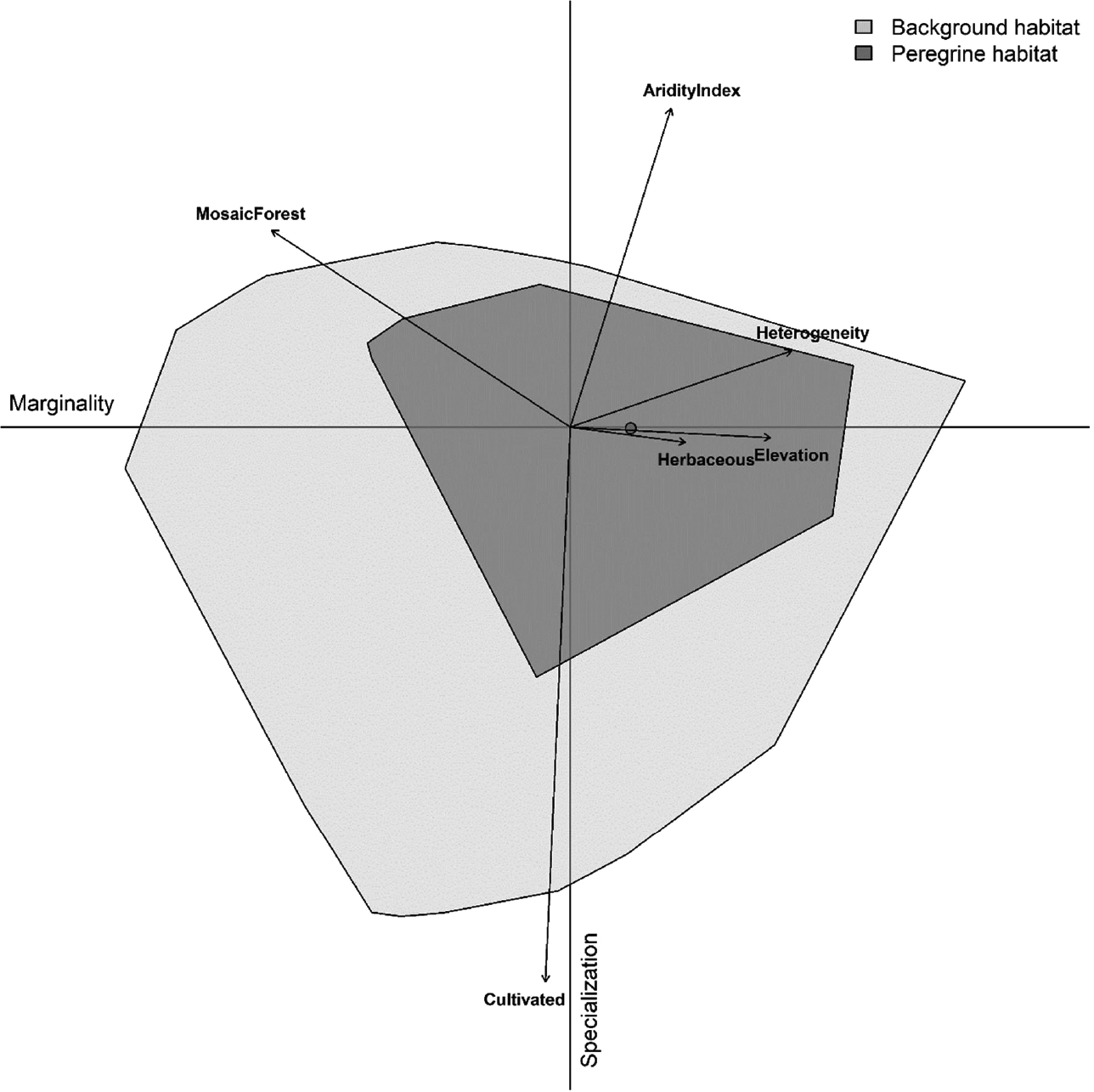
Figure 2. Multivariate resource selection in environmental space using Ecological Niche Factor Analysis (ENFA). Madagascar Peregrine Falcon habitat (dark grey) is represented within the available background environment (light grey) shown across the marginality (x) and specialization (y) axes. Arrow length indicates the magnitude with which each variable accounts for the variance on each of the two axes. The circle indicates niche position (median marginality) relative to the average background environment (the plot origin).
Species Distribution Model
Three candidate models had a ΔAICc ≤ 2, with the best-fit SDM (ΔAICc = 0.00) using linear and quadratic terms and β = 3 as model parameters (Table S2). The optimal model had high calibration accuracy (CBI = 0.847), and was robust against random expectations (pROC = 1.599, SD ± 0.118, range: 1.141–1.920). From the penalized linear beta coefficients, the Madagascar Peregrine was most positively associated with vegetation heterogeneity (1.875), followed by cultivated land (0.018), and highly arid areas (0.012), and most negatively associated with mosaic forest (-0.017). The largest continuous area of habitat extended across the central plateau (Figure 3). A second large area of habitat was identified across the northern Tsaratanana Massif. From the SDM response curves, aridity index had peak suitability at 90%, with highest suitability for areas of increased elevation >1,500 m but with a small prior peak at <50 m elevation (Figure 4). Habitat suitability was highest in areas of high vegetation heterogeneity >0.9, areas with ~30% human cultivated landcover, and <10% of mosaic forest cover.
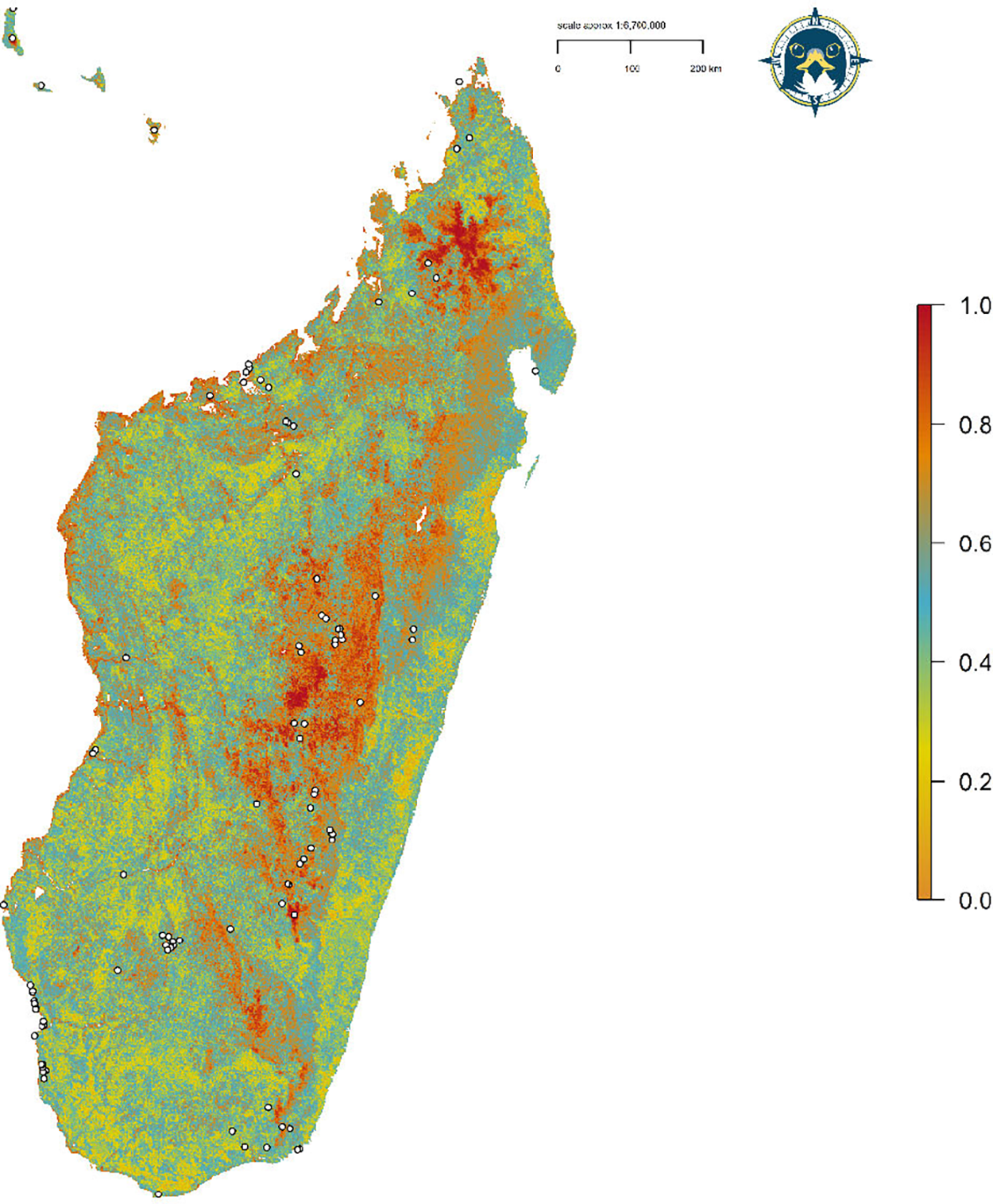
Figure 3. Habitat Suitability Model for the Madagascar Peregrine Falcon. Map denotes cloglog prediction with darker areas having highest habitat suitability. White points define Peregrine occurrences.
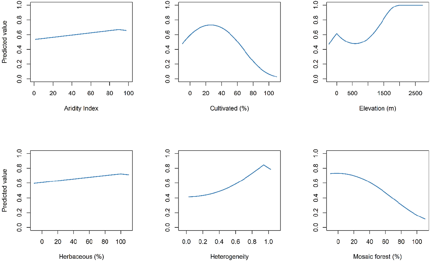
Figure 4. Covariate response curves using penalized logistic regression from the Habitat Suitability Model for the Madagascar Peregrine Falcon
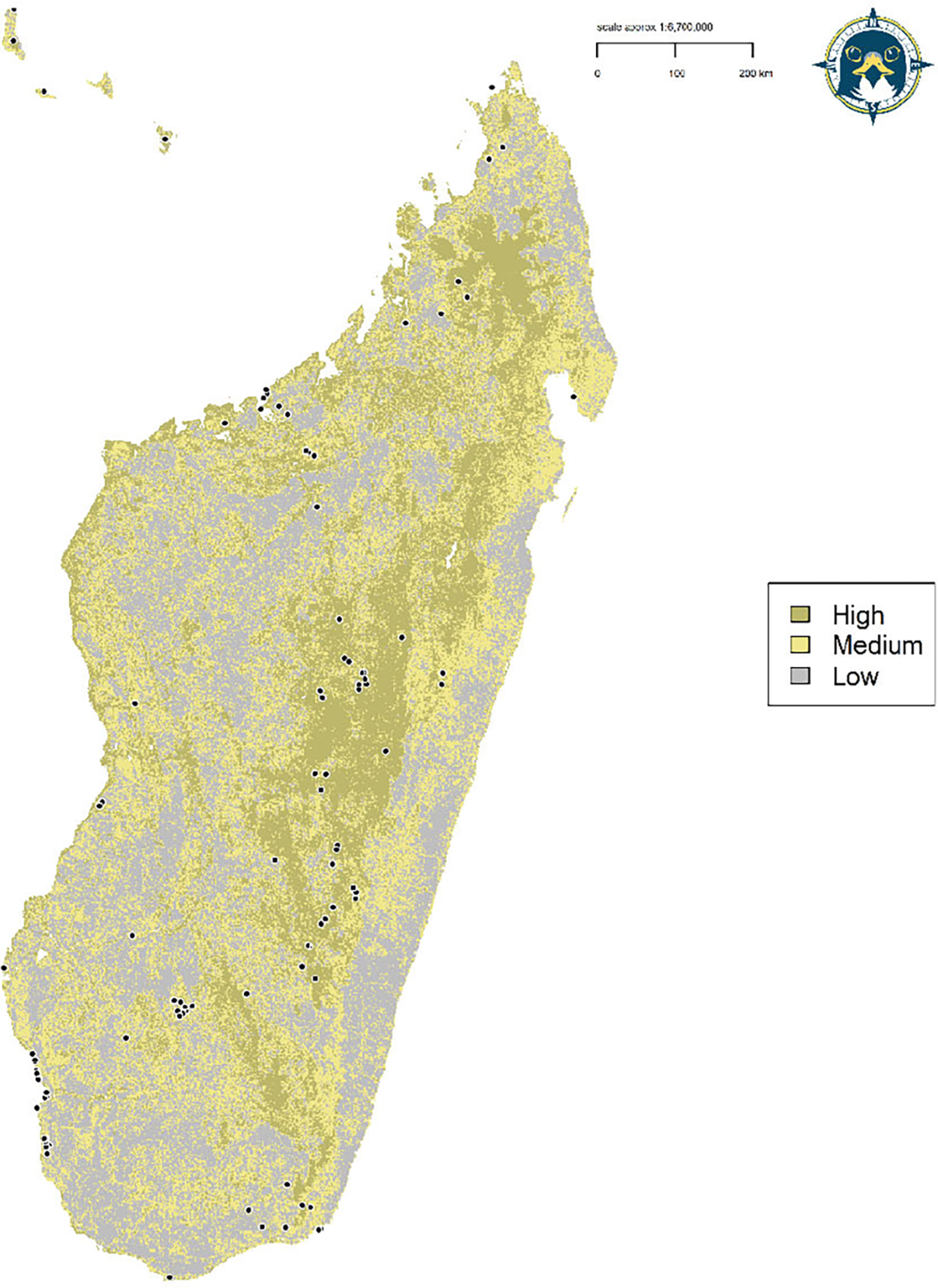
Figure 5. Reclassified discrete habitat suitability model for the Madagascar Peregrine Falcon. Map denotes the continuous prediction reclassifed into three discrete quantile threshold classes. White points define Peregrine occurrences.
Area of habitat and population size
The reclassified binary model calculated habitat in the high quantile class (
 $ \ge $
0.649) totalling 153,265 km2, comprising 26% of the total landscape area (Table 2). Core areas of high-class habitat totalled 37,466 km2, comprising 25% of the total high habitat area. Based on the total area of high-class habitat and assuming pair densities ranging between 500 and 1,000 km2 per territorial pair, we estimate the area of high-class habitat could support 153–307 breeding pairs. From our population estimate the Madagascar Peregrine subspecies would be classed as ‘Vulnerable’ under IUCN Red List criterion D1 with a very small or restricted population numbering <1,000 mature individuals (IUCN Standards and Petitions Committee 2019).
$ \ge $
0.649) totalling 153,265 km2, comprising 26% of the total landscape area (Table 2). Core areas of high-class habitat totalled 37,466 km2, comprising 25% of the total high habitat area. Based on the total area of high-class habitat and assuming pair densities ranging between 500 and 1,000 km2 per territorial pair, we estimate the area of high-class habitat could support 153–307 breeding pairs. From our population estimate the Madagascar Peregrine subspecies would be classed as ‘Vulnerable’ under IUCN Red List criterion D1 with a very small or restricted population numbering <1,000 mature individuals (IUCN Standards and Petitions Committee 2019).
Table 2. Class-level landscape metrics calculated from the reclassified Habitat Suitability Model quantile threshold classes. Area values are in km2.
Discussion
Identifying species ecological requirements is fundamental to understanding species range limits and thus setting conservation planning priorities (Elith and Leathwick Reference Elith, Leathwick, Moilanen, Wilson and Possingham2009, Lawler et al. Reference Lawler, Wiersma, Huettman, Drew, Wiersma and Huettmann2011). Here, we provide the first detailed distribution map for the Madagascar Peregrine Falcon and establish this subspecies’ habitat constraints across its entire range using climatic, topographical, and landcover variables. Our results show predictive models can identify those areas of highest habitat suitability and infer the processes influencing distribution for this subspecies in Madagascar. The core habitat area for the Madagascar Peregrine extends across the central and northern plateau of Madagascar, with patchier habitat around coastal and lowland areas. The Madagascar Peregrine is more likely to be associated with high altitude, arid areas with high vegetation species richness and herbaceous landcover but less likely in areas of cultivated land and mosaic forest. Based on our prediction of high-class habitat, we estimate there could be up to 300 pairs resident throughout their range, and thus the subspecies would be classed as ‘Vulnerable’ under IUCN guidelines.
Previous distribution maps for the Madagascar Peregrine have defined the entire land area across the subspecies range as its distributional limits (Ferguson-Lees and Christie Reference Ferguson-Lees and Christie2005, Sinclair and Langrand Reference Sinclair and Langrand2013, BirdLife International 2019). White et al. (Reference White, Cade and Enderson2013) reduced this to include a distributional area across the far northern and southern ends of Madagascar, and a separate area extending across central west Madagascar, with question marks in between these three areas. Our distribution maps build on these previous estimates, providing both continuous and discrete predictions, and further detail than those previous range maps. We view these range maps as works in progress, and they can be continuously updated as new occurrence data are collected. Indeed, using SDMs to map and update species range limits is gaining in use (e.g. Breiner et al. Reference Breiner, Guisan, Nobis and Bergamini2017, Ramesh et al. Reference Ramesh, Gopalakrishna, Barve and Melnick2017, Da Silva et al. Reference Da Silva, Fernandes-Ferreira, Montes and da Silva2020). Model-based interpolation from community science data offers a cost-effective and convenient method to assess and update the distributional status and range limits for this understudied sub-species, along with broad applications across other data-deficient taxa.
Few species occupy all areas with suitable resources and conditions, with areas of potential presence either occupied by closely related species, or unoccupied due to extirpation or failure to disperse (Anderson et al. Reference Anderson, Peterson and Gómez‐Laverde2002). For the Madagascar Peregrine, the largest area of high-class habitat extended across the central plateau, and further north to a smaller area of high-class habitat in the northern uplands in areas of high aridity. Increased precipitation is known as a strong negative predictor for Peregrine breeding success (Mearns and Newton Reference Mearns and Newton1988, Bradley et al. Reference Bradley, Johnstone, Court and Duncan1997, Anctil et al. Reference Anctil, Franke and Bêty2014) and may explain the positive relationship with areas of high aridity. Across their range the Madagascar Peregrine prefers areas high in species-rich vegetation, which may be a useful proxy associated with increased prey densities in areas of highly heterogenous vegetation (Radeloff et al. Reference Radeloff, Dubinin, Coops, Allen, Brooks, Clayton, Costa, Graham, Helmers, Ives, Kolesov, Pidgeon, Rapacciuolo, Razenkova, Suttidate, Young, Zhu and Hobi2019). Indeed, Peregrine population densities in tropical areas may be restricted by prey resource availability driven by habitat heterogeneity compared to temperate regions (Jenkins and Hockey Reference Jenkins and Hockey2001).
Though the Madagascar Peregrine would likely have evolved over the largely forested island of Madagascar prior to human-driven deforestation (White et al. Reference White, Cade and Enderson2013), elsewhere across their global range Peregrines are generally birds of open, treeless country, feeding largely on other avian species. Thus the strong association with areas of >95% herbaceous landcover in the form of open grasslands, albeit modified by humans, follows the general global trend in Peregrine habitat use with this landcover type (White et al. Reference White, Cade and Enderson2013). Reassuringly, both models identified similar habitat responses in both geographic and environmental space. Whilst the two methods tackle the same problem from different statistical standpoints, the fact both were in general agreement gives credence to the robust nature of our SDM framework to identify habitat preferences. Indeed, the relatively coarse species-habitat associations identified from the ENFA were then further refined by the penalized logistic regression with its ability to define more precise measures of habitat use.
Peregrine pair densities vary widely across their global range dependent on conditions and resources (Ratcliffe Reference Ratcliffe1993, White et al. Reference White, Cade and Enderson2013). Our population size estimate ranging between 150 and 300 pairs based on inferred high-class habitat is similar to a previous estimate for the Madagascar Peregrine which used the entire terrestrial area of their range but with a density of one pair per 2,000–4,000 km2 (White et al. Reference White, Cade and Enderson2013). Estimating population density from SDMs is reliant on having sufficient and accurate occurrence data and selecting the most relevant predictors based on species biology (Franklin Reference Franklin2010, Oliver et al. Reference Oliver, Gillings, Girardello, Rapacciuolo, Brereton, Siriwardena, Roy, Pywell and Fuller2012). Our method here is fairly coarse but gives a first estimate and a baseline from which to develop an integrated approach combining SDMs with population demography. For future range assessments, demographic response studies combined with SDMs are a promising method to further evaluate the relationship between population dynamics and habitat suitability (Bocedi et al. Reference Bocedi, Palmer, Pe’er, Heikkinen, Matsinos, Watts and Travis2014). Further, modelling future distribution with both predicted prey distributions and land cover change may also yield useful insights into the future conservation status for the Madagascar Peregrine.
Our results are reliant on the selected environmental covariates dependent on our definitions – animals may not experience the landscape as humans perceive it. Though we used a range of relevant abiotic and biotic predictors, including predictors derived from satellite remote sensing such as Dynamic Habitat Indices (Hobi et al. Reference Hobi, Dubinin, Graham, Coops, Clayton, Pidgeon and Radeloff2017, Radeloff et al. Reference Radeloff, Dubinin, Coops, Allen, Brooks, Clayton, Costa, Graham, Helmers, Ives, Kolesov, Pidgeon, Rapacciuolo, Razenkova, Suttidate, Young, Zhu and Hobi2019), would further build on the predictive ability of the SDMs presented here. Spatial models have much scope for improvement (Engler et al. Reference Engler, Stiels, Schidelko, Strubbe, Quillfeldt and Brambilla2017, Fourcade et al. Reference Fourcade, Besnard and Secondi2017, Guisan et al. Reference Guisan, Thuiller and Zimmermann2017), but ultimately may also be limited by the amount and quality of occurrence data required (Beck et al. Reference Beck, Böller, Erhardt and Schwanghart2014, Neate-Clegg et al. Reference Neate-Clegg, Horns, Adler, Aytekin and Şekercioğlu2020). Integrating multiple biodiversity data sources would seem a logical evolution for SDMs, particularly within a point process model (PPM) framework (Isaac et al. Reference Isaac, Jarzyna, Keil, Dambly, Boersch-Supan, Browning, Freeman, Golding, Guillera-Arroita, Henrys, Jarvis, Lahoz-Monfort, Pagel, Pescott, Schmucki, Simmonds and O’Hara2019). As shown here, penalized logistic regression, which is mathematically equivalent to a PPM (Phillips et al. Reference Phillips, Anderson, Dudík, Schapire and Blair2017), produces reliable and useful predictions for species range limits in the absence of detailed distributional information for an under-studied raptor subspecies.
Improving our understanding of Peregrine habitat use is especially relevant for conservation because it may point towards potential population change and direct habitat management and protection. Developing a collaborative working relationship with field researchers and land managers feeding back occurrence data would further improve habitat use assessments. In particular, locations of known nest sites would help identify the specific environmental breeding requirements for the Madagascar Peregrine, as the occurrence dataset used here is mainly comprised of sightings. Given the discontinuous range of the Madagascar Peregrine, any breeding habitat studies would be more effective at local, landscape scales. Moreover, developing a participatory modelling process (Ferraz et al. Reference Ferraz, Morato, Bovo, da Costa, Ribeiro, de Paula, Desbiez, Angelieri and Traylor‐Holzer2020), where researchers, planners, and decision makers are all involved in the modelling process would be a significant step forward for raptor conservation in Madagascar.
Species ranges have an invariably discontinuous spatial arrangement, and this most likely applies to all taxa if mapped at fine scales (Ladle and Whittaker Reference Ladle and Whittaker2011). In the absence of human disturbance, discontinuous distributions are a consequence of patchy environments, so it follows that species ranges will follow the latter (Riddle et al. Reference Riddle, Ladle, Lourie, Whittaker, Ladle and Whittaker2011). Range occupancy is also scale dependent, with varying scales of spatial pattern in individual species (Levin Reference Levin1992, Garshelis Reference Garshelis, Boitani and Fuller2000). Refining broad scale modelling to localized regional studies would be a logical next step. Exploratory ground-truthing surveys to validate the models would also be of benefit to conservation managers and modellers alike. Many developing tropical countries lack extensive resources for biodiversity management but are generally the regions of the planet with highest biodiversity. Vast wilderness areas make systematic sampling for many species almost impossible, and that is where spatial models are required to fill knowledge gaps and determine potential distributional areas as demonstrated here.
Supplementary Materials
To view supplementary material for this article, please visit http://doi.org/10.1017/S0959270921000587.
Acknowledgements
We thank all individuals and organisations who contributed occurrence data to the Global Raptor Impact Network (GRIN) information system and the Information Technology staff and Research Library interns at The Peregrine Fund for support. We thank an anonymous reviewer whose comments and suggestions improved the draft manuscript. This work was supported by a funding grant from the M.J. Murdock Charitable Trust.


