


Introduction
The Gravettian (33000–25000 cal BP) is known for its flourishing artwork (e.g. Mussi et al. Reference Mussi, Cinq-Mars, Bolduc, Roebroeks, Mussi, Svoboda and Fennema2000; Jaubert Reference Jaubert2008) and high technological standards, illustrated by the Obłazowa boomerang (Valde-Nowak et al. Reference Valde-Nowak, Nadachowski and Wolsan1987), by ceramics, and by evidence of cordage items, basketry and textiles such as those from Pavlov I and Dolní Vĕstonice (Soffer Reference Soffer, Roebroeks, Mussi, Svoboda and Fennema2000; Soffer & Adovasio Reference Soffer, Adovasio, Svoboda and Sedláčková2004). While cultural life prospered, the Gravettian community had to cope with continuous environmental deterioration. Shortly after 33000 cal BP, summer insolation in northern latitudes started to decline, coinciding with the inception of glaciation processes that culminated in the peak ice-sheets of the Last Glacial Maximum (LGM) (Clark et al. Reference Clark, Dyke, Shakun, Carlson, Clark, Wohlfarth, Mitrovica, Hostetler and McCabe2009). This decline in insolation continued steadily, attaining its lowest level for the entire Upper Palaeolithic shortly after 25000 cal BP (Figure 1). Judging from the δ18O values recorded in the NGRIP GICC05 ice-core (Björck et al. Reference Björck, Walker, Cwynar, Johnsen, Knudsen, Lowe and Wohlfahrt1998; Rasmussen et al. Reference Rasmussen, Andersen, Svensson, Steffensen, Vinther, Clausen, Siggard-Andersen, Johnsen, Larsen, Dahl-Jensen, Bigler, Röthlisberger, Fischer, Goto-Azuma, Hansson and Ruth2006), temperatures throughout most of the Gravettian were lower than in any other period of the Upper Palaeolithic, including the LGM (c. 24000–18000 cal BP; sensu Mix et al. Reference Mix, Bard and Schneider2001). The continuous decrease in solar energy probably led to a progressive decline in net primary productivity and, consequently, to a reduction in animal biomass (cf. Binford Reference Binford2001: 58–113). Together with the advancing glaciers, this trend presumably affected living conditions in higher latitudes particularly strongly.
Figure 1. The climatic conditions during the Gravettian. Temperatures are indicated by the δ18O curve. Insolation (smooth curve) is given in watts per square metre for 60°N. Time on the x-axis is given as cal BP. Data from CalPal 2012 (Weninger et al. Reference Weninger, Jöris and Danzeglocke2012).
The objective of the investigation presented here is threefold: first, we analyse the extent to which climatic conditions affected Gravettian populations throughout Western and Central Europe by estimating absolute numbers of people and population densities for two chronological phases in ten different regions. In contrast to previous palaeodemographic studies, where the Gravettian is treated either as a spatial and temporal unit (Bocquet-Appel & Demars Reference Bocquet-Appel and Demars2000; Bocquet-Appel et al. Reference Bocquet-Appel, Demars, Noiret and Dobrowsky2005), or where internal variability is studied only in smaller areas and with regard to relative values (French & Collins Reference French and Collins2015), our approach allows us to discuss the population dynamics of the Gravettian on a large spatial scale in more detail. Second, we try to assess whether abandonment by migration or local extinction was a more probable cause for the desertion of certain areas during the later part of the Gravettian; and third, we explore to what extent observable population dynamics affected the complexity of the technological and typological spectrum of Gravettian hunter-gatherers.
Material and methods
The database for this study (Maier & Zimmermann Reference Maier and Zimmermann2016) was compiled during an extensive literature survey, and comprises 654 assemblages. Although not necessarily exhaustive, it is considered statistically representative. The chronological boundaries (33000–25000 cal BP) are in good accordance with other chronological definitions of the Gravettian (Jöris & Weninger Reference Jöris, Weninger, Svoboda and Sedláčková2004; Klaric Reference Klaric2008; Jacobi et al. Reference Jacobi, Higham, Haesaerts, Jadin and Basell2010; Kozłowski Reference Kozłowski2015), although slightly older dates are sometimes reported, e.g. from Willendorf II (Haesaerts & Teyssandier Reference Haesaerts, Teyssandier, Zilhão and d'Errico2003).
Temporal division and sorting of the assemblages
We divided the Gravettian into two phases of equal duration: P1 (33000–29000 cal BP) and P2 (29000–25000 cal BP) (Figure 1). This allows for the observation of population dynamics while ensuring a sufficiently large number of assemblages per phase to obtain reliable results. Recorded assemblages were then allocated to one of these phases using both absolute dates and typological data. Absolute dates are available for 219 assemblages, with 146 dated to P1 and 73 dated to P2 (see Table S1 in online supplementary material), an imbalance of 2:1 in favour of P1. The remaining 435 assemblages were allocated according to their artefact typologies. The typological structure of the Gravettian is particularly well suited for such a task, as it comprises a relatively large number of widely accepted, chronologically successive sub-stages, with characteristic typological features. To assess for typological shifts around the chosen threshold of 29000 cal BP, we compiled a set of radiocarbon dates from selected sites with a good chronological control pertaining to the time frame shortly before and after 29000 cal BP (Figure 2 & Table S2). In Western Europe, Bosselin and Djindjian (Reference Bosselin and Djindjian1994) identified six consecutive typological stages for the Gravettian: the Fontirobertian, Undifferentiated Gravettian, Noaillian, Rayssian, Laugerian (A and B) and Protomagdalenian. Prior to or contemporaneous with the Fontirobertian were the Bayacian (Rigaud Reference Rigaud2008) and the Belgian facies called Maisière-Canal (Otte & Noiret Reference Otte and Noiret2007; Jacobi et al. Reference Jacobi, Higham, Haesaerts, Jadin and Basell2010). When reliable radiocarbon dates are taken into consideration (Figure 2 & Table S2), the 29000 cal BP boundary coincides well with the transition from the Noaillian/Rayssian to the Laugerian in Western Europe (Figure 2; cf. Klaric Reference Klaric2008). In Portugal, early and late Gravettian phases occur before and after 29000 cal BP (Bicho et al. Reference Bicho, Marreiros, Cascalheira, Pereira and Haws2015: 500). In Central Europe, the 29000 cal BP threshold roughly marks the transition from the Pavlovian to the Willendorf-Kostenkian (Jöris & Weninger Reference Jöris, Weninger, Svoboda and Sedláčková2004). Typologically, this coincides with the appearance of shouldered points during the later phase (Svoboda Reference Svoboda2007).
Figure 2. Radiocarbon dates from different Gravettian facies and different regions with standard deviation ≤200 around 29000 cal BP (CalPal-Multigroup-compilation with CalPal 2012; Weninger et al. Reference Weninger, Jöris and Danzeglocke2012). As the slope of the calibration curve at around 29000 cal BP is particularly steep, any bias introduced should lead to a ‘peak’ in the summed probability distributions at this position, emphasising the reliability of the observed gaps. n = number of dates included in the sum calibration. P1: 33000–29000 cal BP; P2: 29000–25000 cal BP. For details on dates, see Table S2.
In the valleys of the Prut and Dniester, the appearance of shouldered points (Noiret Reference Noiret2004: 448) and the disappearance of bifacial points (Nuzhnyi Reference Nuzhnyi2009) are seen as fairly precise chronological markers. The earliest 14C dates for shouldered points are reported from layer 7 at Molodova V. Unfortunately, the dating of this layer spans between 30500 and 24500 cal BP (Figure 2 & Table S2). Most dates are, however, younger than 29000 cal BP. When radiocarbon dates from the archaeological horizon with the earliest shouldered points at Mitoc-Malu Galben are taken into account—so-called ‘Gravettian IV’ (Noiret 2009: tab. 7)—the signal becomes clearer, pointing towards an occurrence of shouldered points after 29000 cal BP. Thus it can be stated that around 29000 cal BP, clearly discernible typological shifts may be observed throughout the investigated area, allowing a typological attribution of assemblages to either side of this threshold: P1 or P2. Nevertheless, typological classification is always plagued with uncertainties, and may lead to incorrect allocations. For the reasons explained above, however, in the case of the Gravettian, it is considered reliable enough not to bias the overriding temporal distribution significantly.
Typological attribution increases the assemblages associated with P1 to 347 and P2 to 163, maintaining a ratio of about 2:1. The remaining 144 cases were not attributable by typological means and were excluded from further analysis. They are, however, plotted on our maps for an assessment of potential spatial distortions. For the protocol of demographic estimates, see Maier et al. (Reference Maier, Lehmkuhl, Ludwig, Melles, Schmidt, Shao, Zeeden and Zimmermann2016), and for more details generally, see the online supplementary material.
Results
To account for differences in site density between Western and Central Europe (perhaps caused by different subsistence and land-use patterns), the Optimal Isolines (OIs; comprising areas of equal site densities—for explanations and definition, see the online supplementary material) have been determined individually. For P1, the OI in the western part is found at a radius of 41km Largest Empty Circle (LEC; this serves as a density measure, the larger the LEC, the lower the density—for explanations and definition see the online supplementary material), and at 44km LEC for the eastern part, whereas for P2 it is found at a radius of 50km LEC (west) and 33km LEC radius (east) (Figure S2). The resulting settlement areas, together with the raw material catchments, are depicted in Figures 3 and 4. Departing from these data, population densities have been calculated at both regional and continental scales, resulting in the values given in Tables 1 and 2.

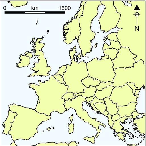
Figure 3. Map of settlement areas and raw material catchments for P1. Black dots: sites attributed radiometrically or typologically to P1; grey dots: sites lacking chronological attribution (excluded from calculations); grey polygons: P1 raw material catchments; red lines (Optimal Isolines): Western Europe 41km LEC radius, Eastern Europe 44km LEC radius (cf. Figure S2).

Figure 4. Map of settlement areas and raw material catchments for P2. Black dots: sites attributed radiometrically or typologically to P2; grey dots: sites lacking chronological attribution (excluded from calculations); grey polygons: P2 raw material catchments; red lines (Optimal Isolines): Western Europe 50km LEC radius, Eastern Europe 33km LEC radius (cf. Figure S2).
Table 1. Regionally differentiated palaeodemographic estimates for the earlier Gravettian (P1).
Notes
Q: quartiles of raw material catchments; OI: selected Optimal Isoline (km); ARM: area of raw material catchments in km² according to Q1–Q3; AOI: area encircled by the Optimal Isoline in km²; Ng: number of groups; P: absolute number of people; Ds: population density (people/km²) within the settlement areas (OIs); Am: area of the considered map section in km²; Dm: population density (people/km²) across the map section.
Table 2. Regionally differentiated palaeodemographic estimates for the later Gravettian (P2). For abbreviations, see notes to Table 1.
The estimated total population for the investigated area (continental scale) ranges roughly between 1700 and 3700 people for P1, and 700 and 1550 for P2. During P1, the highest regional number of people (300–1000) can be found in south-western France, whereas the lowest regional number is estimated for Provence (70–100). The highest density of people (given in people per 100km² (P/100km²)) is estimated for the Prut region (1.7–2.7 P/100km²) and Belgium (1.0–2.5 P/100km²), whereas the lowest density is calculated for the Middle Danube area (0.3–0.7 P/100km²). During P2, the Middle Danube is estimated to have had the highest number (130–460) of people, and the Prut region the lowest (30–110). At the same time, population density in the east (0.5–1.9 P/100km²) seems to have been higher than in the west (0.5–1.0 P/100km²). The median estimates of total population dropped from about 2800 to 1000 people, while the population density within the considered map section (approximately 2000000km²) dropped from 0.0014 to 0.0005 persons per km².
Discussion
Our estimates for the Gravettian indicate low population numbers. Bocquet-Appel and Demars (Reference Bocquet-Appel and Demars2000) and Bocquet-Appel et al. (Reference Bocquet-Appel, Demars, Noiret and Dobrowsky2005) also estimate absolute numbers of people for the Gravettian. The time frame is set slightly differently, ranging from about 31000 to 23500 cal BP and is not further subdivided. Their estimates range between 1879 and 30589 people with an average value of 4776 for Western and Central Europe (Bocquet-Appel et al. Reference Bocquet-Appel, Demars, Noiret and Dobrowsky2005), or 7771 for Western Europe (Bocquet-Appel & Demars Reference Bocquet-Appel and Demars2000), and thus are significantly higher than our estimates, even for the older phase. The generally higher estimates, and particularly the maximum value of about 30500 people, are probably the result of neglecting the empty areas between the site clusters. This, in our view, results in a clear overestimation of the Gravettian population.
Our calculations indicate a reduction in the number of people from P1 to P2 of about 60 per cent. This view is supported by the results of other analyses, such as the study by French and Collins (Reference French and Collins2015) that shows a considerable population decline in south-western France during the late Gravettian. These findings have a strong impact on our view of the Gravettian and thus deserve a critical evaluation. As mentioned above, there is already a strong imbalance in the database between sites attributed to P1 and P2. Before approaching further interpretations, it is thus crucial to discuss possible biases in the compilation of the database that might distort our calculations in favour of P1.
A biased data set?
When only typologically attributed assemblages are considered, there is a ratio of 2:1 in favour of P1. This might indicate a better typological visibility of assemblages of the earlier phase. Indeed, at least in Western Europe, P1 comprises a number of typologically recognisable facies, characterised by several distinctive components, such as Font-Robert points (Fontirobertian), fléchettes (Bayacian), Noaille burins (Noaillian) or Raysse burins (Rayssian). The later phase, however, only includes the Laugerian and Protomagdalenian, whose typological composition is less distinctive. The P2 assemblages may, therefore, be less visible in terms of typology than their P1 counterparts. Assuming, however, that the remaining 144 assemblages, attributable to neither P1 nor P2, are mainly unrecognised assemblages of the later phase seems untenable for three reasons. First, an imbalance between earlier and later Gravettian sites has already been recognised on a regional scale (e.g. French & Collins Reference French and Collins2015). Second, the distinctive types of P1 are not necessarily present in every assemblage, and smaller assemblages in particular probably present a chronologically undiagnostic typological spectrum; the ‘Undifferentiated Gravettian’ of P1 is equally hard to recognise typologically, as are the Laugerian and the Protomagdalenian. Third, if only radiometrically dated sites are considered, then the ratio between P1 and P2 remains at 2:1.
Given that taphonomic loss usually has the effect of younger sites being preserved in higher proportions than older ones (Surovell & Brantingham Reference Surovell and Brantingham2007), the probability of finding sites from P2 should generally be higher than finding sites from P1. This assumption gains further credence given the increased likelihood of P2 sites being preserved as a consequence of the substantial loess accumulation in the later Gravettian. While P1 sites may share comparably favourable preservation conditions, they are more susceptible to becoming deeply buried and thus archaeologically invisible because of their earlier formation. Since typological invisibility does not explain the imbalance in the number of radiometrically dated sites, these observations are a strong argument in favour of a general decrease in the number of sites during the later Gravettian. Therefore, even if P2 assemblages might be less visible by virtue of their typological composition, we consider our database to be statistically representative.
Migration or population breakdown?
Having excluded sampling error as a major factor in the calculation of our estimates, we can now explore their significance for the questions raised at the beginning of the article. In order to assess whether migration or population breakdown (local extinction) led to the abandonment of certain areas, it is necessary to take a closer look at the different regions, as not all areas were affected equally. There seems to be a general trend that settlement areas located farther north and closer to glaciers were more strongly affected demographically.
In Britain, Belgium and the Upper Danube region, the population drops to extremely low levels, and even zero during P2 (see also Straus Reference Straus, Straus, Otte and Haesaerts2000: 76; Jacobi et al. Reference Jacobi, Higham, Haesaerts, Jadin and Basell2010; Pettitt & White Reference Pettitt and White2012: 419–22). In Provence, it drops to a level too low to be measurable using our method. Only in the most southerly settlement area, in Portugal, does the population seem to have remained roughly stable (Figure S3). This geographic variation strongly supports the hypothesis that climatic cooling together with the decrease in insolation were the major factors driving population decline. Given the fact that almost all settlement areas experienced a reduction in population during P2, including those adjacent to areas displaying a complete population breakdown, it must be assumed that people from Britain, Belgium and the Upper Danube area did not leave their settlement areas to migrate southwards, at least not in large numbers. Rather, it seems that populations in these three areas broke down and suffered extinction. Interestingly, a similar conclusion is reached by Roebroecks et al. (Reference Roebroeks, Hublin, McDonald, Ashton, Lewis and Stringer2011) for Neanderthal populations in northern latitudes during the pronounced cooling of MIS 4.
If substantial migration had taken place, a rise in population should be observable in the adjacent areas. The possibility that a few individuals joined neighbouring groups whose overall numbers had decreased despite the arrival of newcomers cannot be excluded. A strong, logistically organised subsistence strategy, predicated on a wide raw material procurement range, and only a few base camps per year, would probably result in an underestimation of the population (Kretschmer et al. Reference Kretschmer, Maier, Schmidt, Kerig, Nowak and Roth2016). The reported raw material catchments do not, however, indicate an increase in size (cf. Figures 3 & 4). Even if they did, it is unlikely that such an increase, even in an extreme case, would result in complete archaeological invisibility in such a way that it might be mistaken for evidence of a population breakdown. Our inference does not mean to imply that hunter-gatherer subsistence would have been impossible under these circumstances, but rather that the ever deteriorating conditions, particularly during the later phase, were a major problem for the adaptive capacities of Gravettian people. Thus, migration does not appear to have been a response of Gravettian hunter-gatherer groups when faced with climatic deterioration. Rather, at many locations the population decreased until eventually it entered a so-called ‘extinction vortex’, i.e. a self-enhancing process, where interaction between different factors such as inbreeding, environmental and demographic stochasticity, and also behavioural failures cause a population to become extinct (Gilpin & Soulé Reference Gilpin, Soulé and Soulé1986).
Observations have shown that some populations decline directly from more than 100 individuals to extinction and that “time-to-extinction scales logarithmically with population size” (Fagan & Holmes Reference Fagan and Holmes2006: 56). There seems to be a trend that “key aspects of a population's dynamics should deteriorate as extinction nears” (Fagan & Holmes Reference Fagan and Holmes2006: 52) because major factors, such as inbreeding, environmental and demographic stochasticity, and year-to-year declines gain importance in small populations. Moreover, observations suggest that a given population size “a few years before extinction was somehow less valuable to persistence than the same population size several years earlier” (Fagan & Holmes Reference Fagan and Holmes2006: 58). Thus, a certain number of individuals prior to or at an early stage of the extinction process can be enough to ensure the survival of a population, while the same number of individuals at a late stage of the process may be too small to prevent extinction.
The surviving hunter-gatherer groups seem to have responded differently. Within all settlement areas in Western Europe, a drop in population density (Ds) is observable, indicating that people were more dispersed across the landscape, perhaps in response to less abundant resources. In the east, however, we see a dramatic drop in density for the Prut region, but, at the same time, a slight increase for the Middle Danube area. The latter could point towards a slight aggregation of the remaining population. The lack of very large sites during P2, such as the P1 sites of Pavlov I, Dolní Vĕstonice I or Předmostí I, which seem to have been settled year-round (Fišáková Reference Fišáková2013), could, however, point to increased residential mobility as a reaction to the altered resource situation.
Minimum viable population and a bottleneck situation
The later phase of the Gravettian seems to have been the rock bottom of demographic development since the arrival of modern humans in Europe (see Figure S4). Given the extremely low number of people in Western and Central Europe (700–1550) between 29000 and 25000 cal BP, it might seem questionable whether this number of people was sufficient to provide a minimum viable population (MVP), i.e. “all members of the population, whether or not they are members of the reproductive age cohort” (Smith Reference Smith2014: 21). The lowest estimate for a MVP for modern humans is set at about 1500 individuals, comprising around 770 individuals in the reproductive age cohort (Hey Reference Hey2005; Smith Reference Smith2014; but see Traill et al. Reference Traill, Brook, Frankham and Bradshaw2010). The effects of inbreeding can, apparently, be avoided even at numbers lower than this: Smith (Reference Smith2014: 19) states that “any population over 100 or so will be sufficient to avoid drift-related inbreeding effects”, although Traill et al. (Reference Traill, Brook, Frankham and Bradshaw2010) see 500 adult individuals as a minimum threshold. The numbers we present are minimum estimates, but despite being relatively low compared to the MVP numbers noted here, our estimates are still within the range of a viable population.
Nevertheless, the dramatic drop in population size certainly led to a loss in genetic variability. This assumption is in accordance with the finding of a genetic bottleneck described by Posth et al. (Reference Posth, Renaud, Mittnik, Drucker, Rougier, Cupillard, Valentin, Thevenet, Furtwängler, Wissing, Francken, Malina, Bolus, Lari, Gogli, Capecchi, Crevecoeur, Beauval, Flas, Germonpré, van der Plicht Cottiaux, Gély, Ronchitelle, Wehrberger, Grigorescu, Svoboda, Semal, Caramelli, Bocherens, Harvati, Conard, Haak, Powell and Krause2016) that led to the loss of mtDNA haplogroup M in the European population. They see this loss as having occurred during the LGM. Our results, however, support the possibility of an even earlier bottleneck, namely during the late Gravettian. The LGM, in contrast, seems to have been a phase of climatic amelioration, with warmer temperatures than during the late Gravettian, increasing insolation, demographic consolidation and renewed population growth (Figures 1 & S3; Maier et al. Reference Maier, Lehmkuhl, Ludwig, Melles, Schmidt, Shao, Zeeden and Zimmermann2016). In particular, south-eastern Spain shows a pronounced increase in population, with estimates of between 200 and 900 people living there during the LGM.
Large-scale and long-distance mating and communication networks can, to a certain extent, counteract the effects of decreasing populations by connecting otherwise small communities to larger meta-populations. People in Western and Central Europe certainly maintained contact with populations in bordering regions. Southern Spain, Italy, the Balkans and the regions north and east of the Black Sea were also inhabited at this time, although the number and density of people seems not to have been very high. Evidence for these networks comes from the female statuettes of that time. Given the striking similarities between, for example, the specimens from Willendorf and Gagarino (e.g. Djindjian et al. Reference Djindjian, Kozłowski and Otte1999: fig. 12.6), located some 1900km apart, communication can be the only convincing explanation, as the probability of equifinality is vanishingly low.
A loss of cultural complexity?
Many studies have pointed out a strong connection between the demographic and cultural evolution of a population (e.g. Shennan Reference Shennan2001; Riede Reference Riede2009; Vaesen Reference Vaesen2012; for an opinion to the contrary, see Collard et al. Reference Collard, Vaesen, Cosgrove and Roebroeks2016). Typological and technological impoverishments have been described for populations that became cut off from their original population, or became otherwise less numerous (e.g. Henrich Reference Henrich2004; Richerson et al. Reference Richerson, Boyd and Bettinger2009; Roebroeks et al. Reference Roebroeks, Hublin, McDonald, Ashton, Lewis and Stringer2011; but see also Collard et al. Reference Collard, Vaesen, Cosgrove and Roebroeks2016). They have also been modelled for a meta-population with frequent extinction of local sub-populations (Premo & Kuhn Reference Premo and Kuhn2010). For the Gravettian, an apparently substantial decline in population during P2 coincided with an impoverishment of the typological and technological spectrum. The evidence for high technological standards almost entirely relates to sites dated to P1. In Central Europe, the spectrum of artisanal craftwork seems to become less complex (Svoboda Reference Svoboda2007: 207), and in Western Europe, there is a trend from easily identifiable typological facies (e.g. Fontirobertian and Noaillian) to apparently typologically simpler assemblages (Laugerian and Protomagdalenian). These observations might indicate a general loss of knowledge and complexity due to population decrease. To the best of our knowledge, there are no quantitative estimates for the complexity of different tools and skills, making it difficult to quantify any associated loss or increase of knowledge over time between phases such as P1 and P2 more meaningfully.
Conclusion
The early Gravettian was a period of cultural and technological prosperity, whereas the late Gravettian seems to have been a period of pronounced crises. The population shrank by about 60 per cent, and a simplification in the material culture that affected typology, technology and artisanal craftwork indicates a broader loss of knowledge. When faced with environmental deterioration, Gravettian hunter-gatherers did not respond by migration. Instead, we observe several breakdowns of regional populations, particularly in the more northerly latitudes. Perhaps as an adaptation to the altered resource bases, people dispersed themselves more widely during the later phase, and exhibited stronger residential mobility, at least in Central Europe. While the later Gravettian seems to have been the lowest point for Upper Palaeolithic demographic development, the LGM was a period of population consolidation and renewed growth. Many aspects of this could only be touched on briefly in this article. It is our hope that future research will allow us to further investigate issues relating to demographic changes during this period: for instance, whether the Heinrich 3 event was the principal trigger for population breakdown, or rather one factor among many others in the process of long-term climatic cooling and population decline; or to find ways to quantify gains and losses in cultural complexity.
Acknowledgements
We thank Jean-Pierre Bocquet-Appel (EPHE, CNRS), Isabell Schmidt, Anja Duwe and Andreea Darida (University of Cologne) for granting access to and compiling data on site distribution and dating; Wei Chu (University of Cologne) for constructive criticism; Jayson Orton for proofreading; and Nicole Bössl (University of Erlangen-Nürnberg) for graphics support. We also thank the reviewers for their constructive comments. This is a publication of the E1 project of the Collaborative Research Center (CRC) 806 of the German Research Foundation (DFG).
Supplementary material
To view supplementary material for this article, please visit https://doi.org/10.15184/aqy.2017.37


