
Introduction
The growing corpus of literature on ancient inequalities incorporates estimates of wealth distribution from widely diverging periods, cultural contexts and data types (e.g. Morris Reference Morris2010; Scheidel Reference Scheidel2017). Non-documentary archaeological sources of evidence are the only means of charting wealth distribution for vast stretches of the human past, and different approaches have emerged (e.g. based on grave goods and house sizes; Windler et al. Reference Windler, Thiele and Müller2013; Kohler & Higgins Reference Kohler and Higgins2016; Kohler et al. Reference Kohler2017; Kohler & Smith Reference Kohler and Smith2018; Porčić Reference Porčić2018). Given the unique potential of archaeological evidence to investigate patterning in inequality over the very long term, there is a clear need for the development of robust measures of wealth inequality that are comparable across differing time periods, cultures, technologies and political systems. Enhancing comparability is also important for interpreting local estimates of inequality in a wider context.
A natural source of methods for addressing these challenges is economics. Simon Kuznets pioneered the comparative and historical study of the total output of an economy measured by gross domestic product (Kuznets Reference Kuznets1965). More recently, Atkinson and Piketty (Reference Atkinson and Piketty2007) used measures of the share of total income received by the richest members of a society to study economic inequality from the early twentieth century onwards. Notwithstanding the limits of single indicators of complex and multidimensional phenomena, these simple measures have provided an indispensable lens for the comparative study of modern economies.
Their deployment in archaeological studies, however, raises a number of challenges. First, much of the above work is based on a complete enumeration (e.g. using census or tax authority data) of the relevant populations; archaeological studies necessarily rely on samples of data, which are often quite small and with unknown statistical properties. Second, most economic measures use market prices as a common indicator of value for aggregating the heterogeneous elements that constitute total output or a living standard. In most archaeological applications, no similar method of aggregation is feasible. Finally, the range of societies that economists typically consider is substantially more homogeneous in culture, social structure and technology than those studied by archaeologists.
While interest in inequality may derive from concerns about disparities in living standards (measured by income), these are often difficult to measure with the data available to archaeologists. More readily available information on wealth provides both an indirect indicator of income, and a measure of the wealth-holder's social and economic status. Wealth is defined as a stock of assets—housing, livestock or land, for example—that yields a flow of income or other contributions to an individual's or family's well-being. Here, we propose methods for the measurement of wealth inequality using archaeological data, allowing the exploration of economic disparities in a far greater range of social structures and economic systems. Building on recently collated datasets for quantifying ancient wealth inequality, we provide estimates for 150 Eurasian and North and Central American site-phases, ranging in age from 23 000 years ago to the eighteenth century AD.
Some of the dimensions by which we measure inequality are best conceived of as individual attributes: that is, something that people simply have more or less of, such as height. Other dimensions, however, are best conceived of as an aspect of relationships between people, measured by differences in some attribute. Inequalities in wealth among households belong in this latter class.
The Gini coefficient is a measure of wealth inequality that can be compared across societies and types of wealth. It ranges from zero (complete equality) to one (all wealth is held by one person), and is defined as one half of the mean of the differences among all pairs of households in the population, divided by the mean wealth in the population. Partial measures of inequality, such as the proportion of all wealth owned or income received by some small fraction of the population, are used widely in measuring wealth inequality, as they are sometimes available in written tax or probate records. In contrast, the Gini coefficient is a measure of inequality in the entire distribution of wealth (see also the online supplementary material (OSM)).
A major challenge to comparative research on ancient wealth inequality is that the relevant information from various sites and phases is based on different sample sizes and methods. Moreover, such information pertains to different indicators of wealth (e.g. dwelling or storage area size, or grave goods), may omit measurement of those without wealth, such as slaves, and derive from populations of vastly differing size, such as a city or a small hamlet. Here, we develop methods for using such heterogeneous data to produce estimates that are comparable across sites and periods. Cross-cultural research has an important place in archaeology (Bogucki Reference Bogucki1999; Trigger Reference Trigger2003), not least in that it informs long-term perspectives on contemporary dilemmas—growing economic inequality being a prominent example. We aim to show that the methods of comparability proposed here offer superior insight compared to the collation of available Gini coefficients without regard to the heterogeneous underlying information on which they are based.
There is a limit, however, to what can be inferred even on the basis of comparably measured indicators of material wealth inequality. Two societies with equal wealth inequality by our measures may differ substantially in social complexity, political hierarchy, disparities in consumption, economic injustice or other dimensions associated with the term ‘wealth inequality’. For example, while the evidence is indirect, many of the societies under consideration may have practised systems of wealth redistribution with the result that inequalities in consumption were less than wealth inequality. Furthermore, our measures do not directly inform about political inequality and how this may differ, for example, between stateless and state-governed populations.
Two identical Gini coefficients measuring wealth inequality may even be associated with radically different distributions of wealth—for example, one in which inequality arises from a small concentration of entirely property-less households at the bottom of an otherwise relatively equal (in terms of wealth) population and the other with a few exceptionally rich households in a population of small landowners (e.g. see the OSM). Thus, sometimes the same Gini coefficient value can be associated with very different outcomes in relation to the dimensions that are not directly measured.
The dataset
The archaeological data incorporate a series of regional datasets assembled by other scholars, plus additional sites with accessible data of particular interest for assessing questions of inequality. All of the sites are listed in the OSM. Geographically, they are distributed across Eurasia, North America and Mesoamerica; chronologically, they range from a single observation at 23 000-year-old Ohalo II in the southern Levant (Nadel Reference Nadel2003) to eighteenth-century AD communities of the Pacific Northwest (Schulting Reference Schulting1995; Prentiss et al. Reference Prentiss, Foor, Murphy, Kohler and Smith2018). Where possible, we distinguish chronological phases within site sequences in order to avoid combining distinct periods of occupation.
Two of the archaeological datasets—for the Columbia Plateau and Hohokam—offer large, multi-site data on grave goods in individual burials (McGuire Reference McGuire1992; Schulting Reference Schulting1995). We use these datasets, chosen for their size and disparate cultural contexts, to develop some of our adjustments to wealth-distribution estimates below. To the same ends, we also incorporate historical datasets on land ownership in a large agricultural population during the seventeenth to eighteenth centuries AD at Krummhörn in Germany, on the distribution of household wealth in 1427 Florence, Italy, and on regional inequality from medieval Finland (Herlihy & Klapisch-Zuber Reference Herlihy and Klapisch-Zuber1985; Nummela Reference Nummela, Lamberg and Haikari2011; Willführ & Störmer Reference Willführ and Störmer2015).
Our unit of analysis for assessing wealth distribution is the household. We define ‘households’ as co-residential groups occupying modular architectural units with standardised features that suggest redundancy of domestic functions among units. Multiple units may cooperate as a larger household group, but the widespread archaeological observation of standardised domestic units suggests that they often acted as fundamental social agents. Moreover, although wealth may sometimes be shared across households, systematic wealth-sharing takes place within the house; the house can be defined as a physical (and metaphorical) unit for storing and sharing wealth (Gudeman & Rivera Reference Gudeman and Rivera1990).
From individual to household inequality in grave goods
As household membership typically cannot be identified from burial remains, we calculate a between-household inequality measure. From the burial sites of the Columbia Plateau (Schulting Reference Schulting1995) and the Hohokam Culture (McGuire Reference McGuire1992), we identify those with the greatest number of sex-identified observations. For these four sites, we first compute the Gini coefficient of individual wealth, among only the individuals whose sex is identified. Second, we estimate the Gini coefficient of couples’ wealth, where hypothetical couples are created assuming perfect wealth assortment—that is, the richest females are matched with richest males, and the poorest females with the poorest males. Couples’ wealth is then the sum of the wealth of the matched individuals. Third, we compute and average 10 Gini coefficients on couples’ wealth, with couples generated assuming random assortment—that is, males and females randomly matched, irrespective of wealth. Table S1 in the OSM presents the results. Fourth, our estimate of between-household inequality is the average of the results of the two methods: perfect assortment and the absence of assortment. The ratio of the Gini coefficients estimated for the hypothetical couples to the coefficients estimated from individual data is 0.90 and 0.92 for the Columbia Plateau and Hohokam, respectively (Table S1). In subsequent adjustments, we use the mean value, 0.91.
A robustness test of our method is possible using a small ethnographic dataset of the wealth of actual couples. Thus, we can test whether the estimated Gini coefficient for hypothetical couples obtained through our method is close to the Gini coefficient computed on the observed wealth of real couples. In the OSM, we find that the two estimates are similar. The fact that the three estimates—two archaeological and one ethnographic—are very similar encourages our application of this method to the other archaeological cases in our dataset.
Sample size and the Gini coefficient
As the fundamental data underlying the Gini coefficient are wealth differences among pairs of households, in principle the coefficient can be calculated for a population, or sample, as small as two households. Here, we explore the statistical properties—bias and imprecision—of estimates of a Gini coefficient for wealth, based on small samples of m observations from a (sometimes unknown) number M in the total population. The question of interest is: if we recover data on m individuals in an estimated total population of M individuals, what is the nature and magnitude of the biases and imprecision affecting Gini estimates, and how do larger sample sizes attenuate these biases and the imprecision of the estimates?
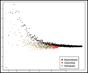
Using a dataset with observations of individual wealth ownership, we assume that the total number of observations, M, is the total population and the Gini coefficient computed on M is the true Gini coefficient. We then hypothetically restrict the dataset to a number of individuals m<M, and then estimate the Gini coefficient that would have resulted. To do this, we first set m = 2, then randomly select a pair from the dataset and, on this basis, we calculate a Gini coefficient. We conduct this process of sampling with replacement for m = 2 a thousand times, which produces a mean estimate and its standard error. We repeat this for all values of m< M. We then implement the algorithm on three large datasets from both archaeological and historical records: the entire burial wealth dataset from the Columbia Plateau and from the Hohokam society at la Ciudad, and the records of land ownership in the large seventeenth- to eighteenth-century agricultural population at Krummhörn, Germany.
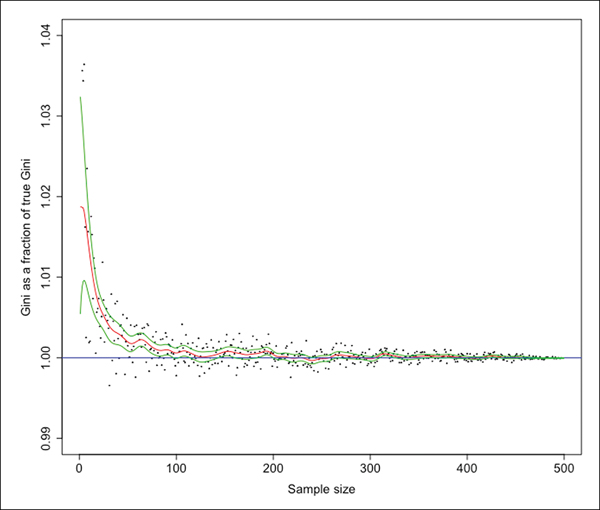
The results are shown in Figure 1. Panel ‘a’ shows that bias is substantial when the sample is very small, and it quickly approaches zero as the sample size m increases. Neither skewness nor total population size (M) appear to affect the extent of bias in this case. Panel ‘b’ shows that the standard errors of the estimated Gini coefficients—as a fraction of the true Gini coefficient—are strikingly small, even for samples of modest size. That the relationships in Figure 1 are very similar, despite being based on very different cultural contexts, suggests that our statistical method has wider applicability across our heterogeneous dataset.
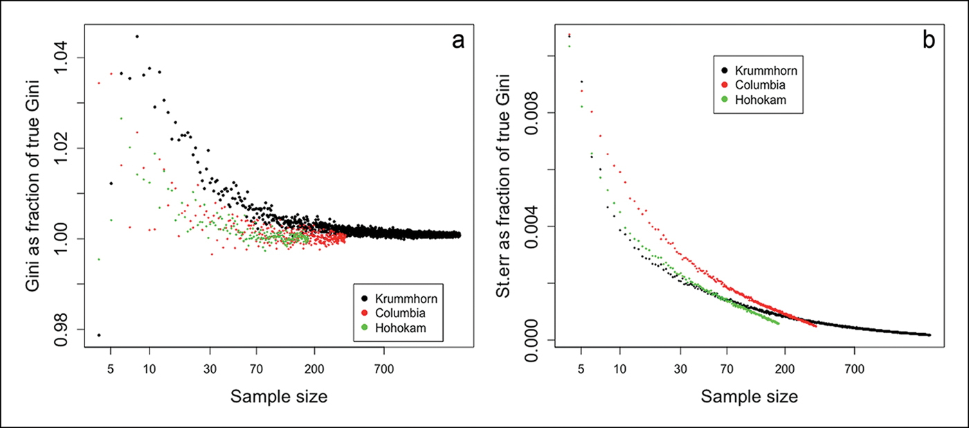
Figure 1. Sample bias and standard error of the Gini coefficients in three large datasets. The (a) and (b) panels, respectively, show the estimated Gini coefficient as a fraction of the true Gini, and the standard errors of the estimated Gini coefficients as a fraction of the true Gini, for Columbia Plateau (red dots), Krummhörn (black dots) and Hohokam (green dots). The x-axis is ratio-scaled (figure by the authors).
Adjusting Gini estimates for sample bias
To adjust downwards the Gini coefficients that are upward-biased due to small sample size, we use the Columbia Plateau dataset shown in Figure 1 and estimate a non-parametric relationship between the bias and the natural logarithm of the sample size. The adjustment would not be appreciably different had we used the other datasets, given the very similar relationships of sample size and bias shown in Figure 1. Figure 2 summarises the relationship between the two variables using a local polynomial regression. For each Gini coefficient in our dataset, we use the number of observations in our data to predict the sample bias, in order to estimate the size of the Gini that would have been estimated had the entire population been observed. This procedure does not require us to know the true population size, as the extent of bias becomes very small for samples of modest size, irrespective of M.
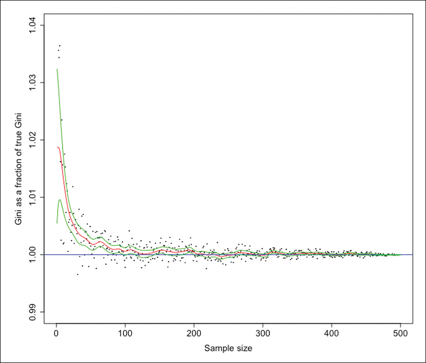
Figure 2. Non-parametric regression for sample bias. The estimated Kernel regression (red line) of the ratio of the estimated Gini to the true population Gini (black dots) on the population level. The bandwidth is equal to 5. The confidence intervals (green lines) are also shown, derived as plus and minus twice the standard error (figure by the authors).
Accounting for those without wealth
Due to data limitations, estimates of Gini coefficients often omit relevant ‘zeros’: that is, those people with none of the attribute being measured. Inequality of land ownership, for example, is often mis-measured by a Gini coefficient on the holdings of landowners because it excludes the landless. Similarly, while estimates of inequality of grave goods in southern Mesopotamia and Roman Italy (Stone Reference Stone, Kohler and Smith2018) include those without wealth among the free population, they exclude the slaves who lived and worked in the urban centres. Thus, these exclusions understate substantially the degree of wealth inequality in a population.
To include those groups without access to specific resources (the missing ‘zeros’) requires two pieces of information. The first is an estimate of how numerous these missing zeros are, which we can establish from historical sources about the populations in question (see the OSM). The second is an estimate of the effect of excluding the zeros on the Gini coefficient, which we obtain by manipulating a mathematical expression for the Gini coefficient in a class-divided economy. In the OSM we show that an approximation of the true Gini coefficient (G) based on an observed estimate (G′), calculated from a dataset with a fraction u of the total population without wealth not used in the estimate (so u is the fraction of missing zeros in the total population), is:
 $$G = {G}^{\prime} + u-u{G}^{\prime}.$$
We use this equation, along with an estimate of u, to calculate the true Gini coefficient, and check the validity of this approach by the same methods already introduced to estimate the effects of small sample size. We study populations for which we know the entire wealth distribution and from which we can hypothetically remove the zeros and then compare the true estimates with our estimates based on the hypothetical absence of data on the zeros using equation 1.
We use 32 distributions of different forms of wealth: grave goods of 23 burial sites from the Columbia Plateau and four from the Hohokam Culture; the distribution of household wealth in 1427 Florence; and four cross-sections of seventeenth- to eighteenth-century land ownership in Krummhörn, Germany. Table S3 shows the data used for the analysis. To check our method, we estimate for each population the Gini coefficient of the whole distribution using the known fraction of zeros, and the Gini coefficient estimated on the hypothetical population for which the zeros have been removed.
The mean absolute error between the estimated and the true Gini on the total population as a fraction of the mean true Gini is 0.012, and the correlation coefficient between the two sets of values is 0.99. These results suggest that our method is reasonably precise, and it provides the basis for our upwards adjustment of the Gini coefficients with missing zeros. As a further check, we use a least squares regression to predict the true (entire population) Gini coefficients using the values of G′, u and uG′ derived by hypothetically removing zeros from these populations. As predicted from equation 1, the estimated regression coefficients are almost exactly one (for the first two) and minus one for the product. We describe how we estimated the numbers of those excluded—landless slaves in the case of southern Mesopotamia and Roman Italy—in the OSM.
Comparability among different asset types
Some asset types tend to be more equally distributed than others. In modern societies, for example, housing is much more equally distributed than ownership of companies. If we want to compare the inequality of household wealth in different societies, we first need to assess how the distribution of the asset that is available to measure inequality in a specific society compares to the distribution of the other forms of wealth constituting household wealth.
We have estimated wealth inequality using the following four measures: land, house storage space, house living space and grave goods. Determining what counts as wealth is a critical issue. In agricultural societies—even in the small-scale, labour-intensive examples included in our dataset—informal property rights in land probably existed, and the main source of well-being for a household was the land it cultivated. For this reason, when both living and storage spaces are clearly identified, we use only storage area—indicative of access to land—as a proxy for household wealth. For many archaeological sites, however, living and storage areas have not been distinguished. In these cases, we use the total house area as a proxy of household wealth. For some agrarian societies, household wealth inequality is measured directly through land inequality. In these cases, given the primary function of land for the production of household well-being, we consider it the measure of household wealth.
We consider grave goods not as a form of wealth, but as a costly signal, conveying information about the status and wealth of the deceased. While the goods that are included in burial assemblages may sometimes be objects representing an individual's or group's wealth—tools, weapons, animals and valued household objects, for example—grave goods may also be entirely symbolic and non-utilitarian. What matters for our purposes is that, whatever their form, burial goods are an indicator of the wealth of the household of the deceased, as the household must forgo some of its wealth to provide grave goods to accompany the burial.
There are both reasons and evidence to support the hypothesis that grave goods are more unequally distributed than forms of wealth, such as indicated by dwelling size (see the OSM; Peterson & Drennan Reference Peterson, Drennan, Kohler and Smith2018). In southern Mesopotamia during the Neo-Babylonian period, for example, Gini coefficients for house area (living and storage space) and grave goods are 0.621 and 0.878, respectively (corrected by sample bias, couples and missing zeros, as explained in the previous sections).
We reconcile these two wealth types—house area and grave goods—using archaeological datasets for which inequality is measured in the same society and in the same time period, for both asset types. For the cases in which the two measures are available (Table S5), the inequality in house area—indicative in this case of household wealth—is on average 71.9 per cent of the inequality in grave goods, with a remarkably small standard deviation of 4.7 per cent. From this, we infer that, were household wealth data available for those societies on which we have data on grave goods only, the inequality in the latter would be approximately three-quarters the inequality in the grave goods. Therefore, in our analysis, a Gini coefficient measured on grave-good inequality alone is reduced by 28.1 per cent of its value to make it comparable to inequality in household wealth.
Scale effects: comparability across different population sizes
Suppose that we have data on a single ‘village’, but to achieve comparability of scale with our other estimates, we would like to estimate the degree of inequality in the ‘district’ of which that village is a part, along with the other villages making up the district, but on which we do not have data. Taking wealth inequality in the ‘village’ as an estimate of wealth inequality in the entire ‘district’ will not produce comparable estimates, as we expect that larger populations will be more heterogeneous geographically, demographically and even institutionally and culturally, and hence may exhibit greater levels of wealth inequality. We observe that this is the case in our measures of inequality of grave goods on the Columbia Plateau; the Gini coefficient for the entire population in the late prehistoric phase is 0.647, while the average of the Gini coefficient for the six burial sites from the same phase is 0.573.
To achieve comparability of scale, we use an estimate of the population-size effect to infer the Gini coefficient for the population at a given benchmark size. The method is based on comparisons of Gini coefficients for lower-level population entities and the larger entities that they constitute. We call this the ‘nested method’. The advantage of the nested method is that we are able to estimate the size effect for population groups that are probably similar in most respects other than size because the larger unit is composed of the smaller units. It provides a far more accurate estimate of the pure scale effect than is possible using non-nested data—namely, by comparing Gini coefficients across populations of differing sizes.
Three datasets allow us to estimate the difference between the Gini coefficient for the constituent lower-level units and the Gini for the higher-level unit that is the composite of all of these: the datasets from the Columbia Plateau and Hohokam Culture, and one dataset from 1571 Finland (Nummela Reference Nummela, Lamberg and Haikari2011). The latter represents a pre-industrial dataset of wealth distribution with complete geographic coverage; each upper administrative unit is the composite of all the lower ones.
In the OSM, we use the Columbia Plateau dataset to explain how the scale effect is computed. The scale effect is illustrated in Figure 3a by the slope of the line connecting the Gini at the site level (the smaller entity) to the Gini of the entire population made up of these six sites. Figure 3b compares the scale effects for all of the phased Columbia Plateau sites with those of the Hohokam sites, and shows that, as the population of the lower-level entity increases, the scale effect—represented by the slopes of each point in the figure—decreases.
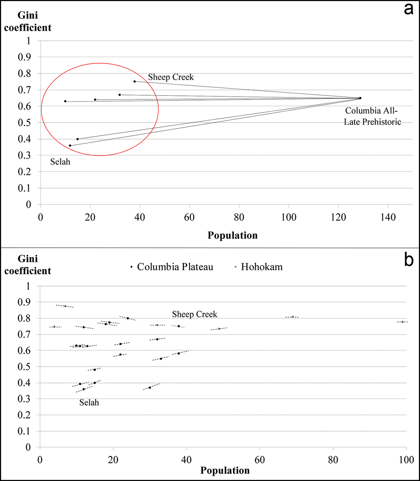
Figure 3. Examples of scale effect for Columbia Plateau and Hohokam Culture sites. Panel ‘a’ shows the Gini coefficients and population size for each site of Columbia Plateau in the late prehistoric phase (dots inside the red circle) and the Gini coefficient and population size at the regional level in the same phase. Panel ‘b’ shows the scale effects for each burial site at the Columbia Plateau excavation (black dots) and at the Hohokam excavation (grey dots). Here, the scale effects are the slopes of the line segments at each point, illustrated in ‘a’ by the slope of the line from the lower-level entity to Columbia (figure by the authors).
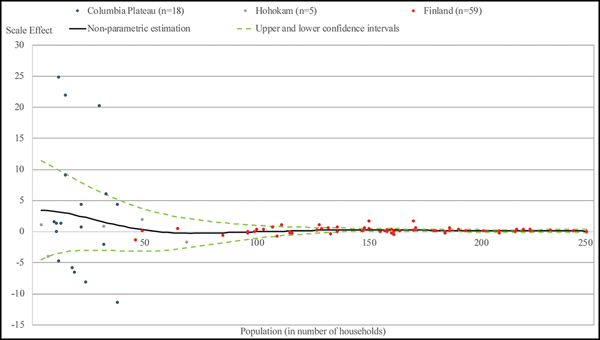
To ensure coverage over the entire range of relevant population sizes, we merge the three datasets with the scale effects measured at lower levels with population smaller than 250 households (Columbia Plateau, Hohokam and late medieval Finland) and plot, in Figure 4, the relationship between the scale effect (multiplied by 1000) and the population of the lower units at which it was computed. We observe that, for very small populations, the scale effect is substantial and, as population increases, a very sharp decline in the scale effect occurs; beyond a population size equal to about 50 households, the scale effect is close to zero. We develop a statistical summary of these data that allow us to scale-adjust the Gini coefficient for any population size.
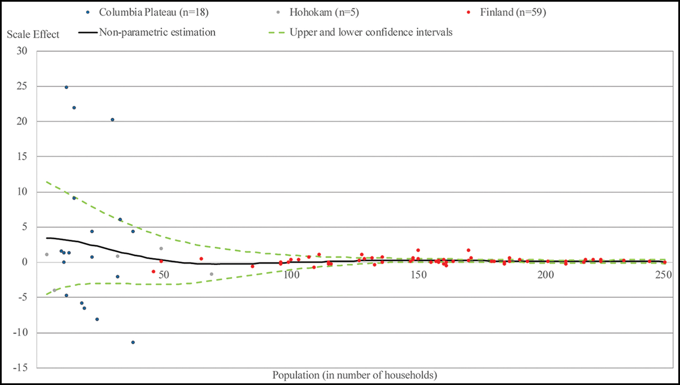
Figure 4. Scale effect estimated from Columbia Plateau, Hohokam and Finland datasets and kernel regression. The scale effects estimated from the Columbia Plateau (blue dots, n = 18), Hohokam (grey dots, n = 5) and Finland (red dots, n = 59) datasets and the non-parametric relationship between the scale effect and the population level (black line). The confidence intervals (dashed green lines) are also shown, derived as plus and minus twice the standard error (figure by the authors).
The estimated scale effects at each population level are used to derive a function reflecting what we call an ‘estimated pure scale effect’, showing how the Gini coefficient varies over the range of population sizes for reasons of scale alone. For the purposes of our adjustment, what matters is its slope, rather than the value of the Gini coefficient for any population level. We arbitrarily choose as a starting value of our function a Gini coefficient equal to 0.5 at the benchmark population level equal to 50 households. From this arbitrary benchmark and the estimated slopes in Figure 3b, we construct the estimated pure scale-effect curve in Figure 5.
Figure 5. Scale adjustment to a common population level. An example of scale adjustment when the actual population is smaller than the benchmark population level (50 households). The example is the adjustment of the Gini coefficient for Neolithic Vaihingen (Germany, sixth millennium BC), where the original Gini was estimated on 11 households. The adjustment works in the same way when the raw Gini was estimated on a population larger than the baseline (figure by the authors).
Figure 5 shows how the function is used to size-adjust the observed Gini coefficient for Neolithic Vahingen, Germany (after the correction by sample bias, 0.189) estimated from a population of 11 households. We let gi be the observed Gini, g i(50) the size-corrected Gini, g(11) the predicted Gini for population size equal to 11 households and g(50), the predicted Gini for population size equal to 50 households. The figure also shows that the resulting scale correction, equal to the difference between g i(50) and g i, is 0.007. We can assess the accuracy of our method by the following thought experiment. Suppose there are M a large number of lower level entities ‘villages’ that make up a district, and we have evidence on m<M of these—that is, some, but not all, of the villages. How accurate a prediction of the inequalities at the district level is possible using our estimated pure scale-effect function estimated from our three datasets and shown in Figure 5? Using the largest set of lower-level entities from the Columbia Plateau dataset (M = 10) to predict the district-level inequality, we find that when we use all 10 of the data points, the error is 0.04. The average error across multiple random picks of four lower entities is equal to 0.06, a number that is reassuringly close to the case of M = 10.
Results
Figure 6 shows the relationship between the Gini coefficients entirely unadjusted for comparability and the fully adjusted estimates. Where adjustments have been limited to taking account of population and sample size, the final estimates are quite similar to the unadjusted ones; except for very small populations and sample sizes, our estimated biases are quite modest. By contrast, the adjustments for estimates based on grave goods (downwards—that is to the right of the 45° line in the figure), or for excluded slaves and other households without property, the adjustment (upwards—that is to the left of the 45° line) are substantial. The average absolute value of the adjustment is 15 per cent of the value of the raw Gini coefficient, suggesting that unadjusted measures are, in general, quite unreliable.
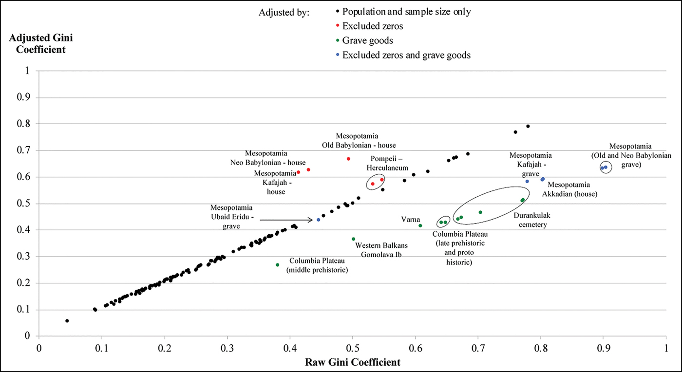
Figure 6. Comparing the raw and adjusted Gini coefficients. The relationship, for each case, between the raw Gini coefficient (horizontal axis) and the Gini coefficient after all the adjustments (vertical axis). The black dots are the estimates adjusted by population and sample size only, while red, green and blue dots are the estimates that have also been adjusted by, respectively, the missing fraction of zeros, the grave goods or both adjustments (for sources, see the OSM) (figure by the authors).
The 150 adjusted Gini coefficients included in our dataset show a wide heterogeneity in the level of inequality from archaeological sources (Figure 7), ranging from around 0.1 to almost 0.8. Elsewhere, we use these data to provide an interpretation of the increase in wealth inequality in Western Eurasia up to the early first millennium AD (Bogaard et al. Reference Bogaard, Fochesato and Bowlesin press).
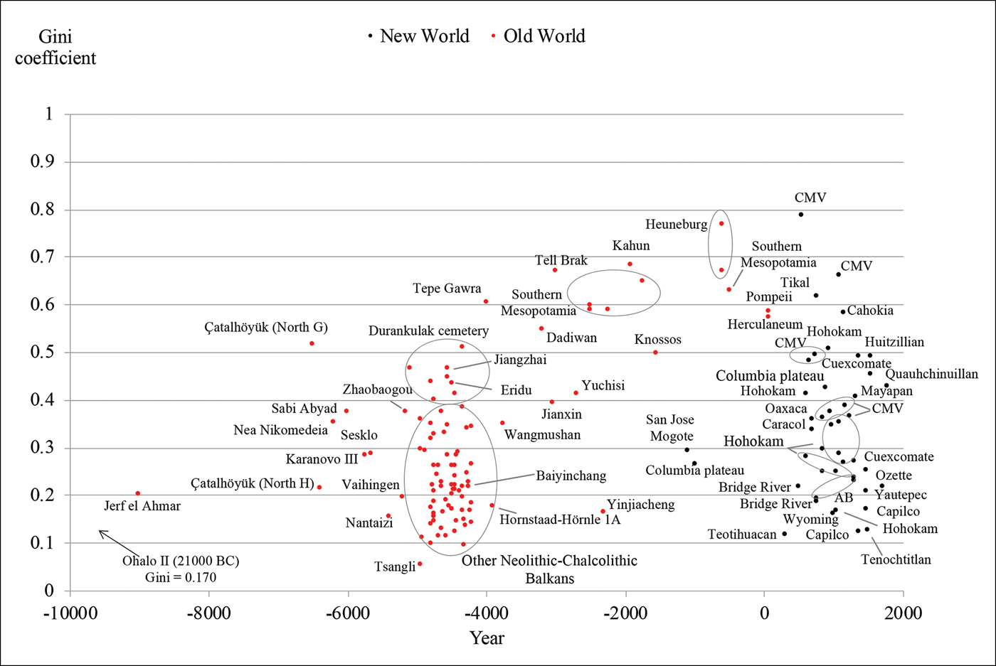
Figure 7. Wealth inequality from archaeological data. The Gini coefficients in the 150 societies included in the dataset, after the adjustments described in the previous sections (CMV = central Mesa Verde; AB = American Bottom) (for sources, see the OSM) (figure by the authors).
Discussion
We have sought to measure wealth inequality in ways that make it substantially comparable across diverse economies, cultures and time periods. In some respects, the results are promising. Our demonstration that relatively small samples from much larger populations yield reasonably accurate and precise estimates of the Gini coefficient is encouraging, especially for archaeologists and others unavoidably constrained by the feasibility of generating more inclusive samples. But the underlying assumption that what is ‘found’ and what is ‘missing’ in the archaeological record is random rather than systematic is likely to be violated in practice. Where there is a clear bias towards, for example, the excavation of larger houses, as at Knossos (see the OSM), or the exclusion of slaves and other households without property, our adjustments have addressed the bias as adequately as the current data allow.
Our methods of approximation of the total population Gini coefficients from estimates where those without wealth are missing also appear to be surprisingly accurate. Similarly, our estimates of wealth inequality among couples hypothetically constructed from the burials of individuals are consistent across two archaeological sites and replicated almost exactly using a sample (albeit small) for which complete data are available.
In another respect, however, our results highlight uncertainties. We lack prices or similar valuations as a method of establishing comparability across types of assets, such as housing vs grave goods, for example, or even among differing indicators of similar assets—that is, the heterogeneous objects making up our measures of grave goods. In the latter case, we have used systems of relative grave-good values adopted by the archaeologists who initially described the data. In the former case—comparing distinct asset types—we have used a relatively small number of datasets in which more than a single dimension of wealth has been measured. It is reassuring that the estimates on which these conversions are made—grave-good inequality to house inequality—are very similar across datasets, and that grave-good inequality is very highly correlated with house-size inequality (suggesting that the former is informative about the latter). Moreover, our measures are necessarily incomplete. We have not, for example, measured the human wealth of slave owners, which in some societies in our sample (e.g. southern Mesopotamia) would constitute a considerable fraction of total wealth. We have also not attempted to incorporate a systematic measurement of livestock wealth.
These uncertainties and gaps, while substantial, should not be exaggerated. We cannot, for example, think of any plausible adjustment in the data that would alter the impression from Figure 7 that Western Eurasian Neolithic populations demonstrate considerably less wealth inequality than many later examples. Similarly, there are no plausible adjustments that would change the result that post-Neolithic wealth inequality in Eurasia tended to be higher than inequality in the Western hemisphere. We have thus shown that more systematically and comparably measured indicators of wealth disparities do not overturn, and indeed reinforce, the primary finding of Kohler et al. (Reference Kohler2017): that high wealth inequality was more persistent over the long term in Eurasia than in North America and Mesoamerica prior to European contact.
Acknowledgements
Thanks to Paul Halstead, Rick Schulting, Todd Whitelaw, Chiaki Moriguchi, seminar participants at the Hitotsubashi University Institute of Economic Research, participants of the 2017 Oxford short course on long-term inequality, and two anonymous reviewers for insightful comments. Thanks also to Marko Porčić for his unpublished database of Balkan Neolithic–Chalcolithic house sizes; to Kai Willführ and Eckart Voland for providing the updated Krummhörn dataset; to Ilka Nummela for providing the late medieval Finland dataset; and to the Dynamics of Wealth Inequality Project, Santa Fe Institute, for support and hospitality.
Supplementary material
To view supplementary material for this article, please visit https://doi.org/10.15184/aqy.2019.106