


Introduction
Terra Nova Bay (TNB) is located in the western sector of the Ross Sea, along the Victoria Land coast. It occupies an area of about 6000 km2 delimited by the Drygalski Ice Tongue to the south and Cape Washington to the north (Fig. 1). The continental shelf is one of the deepest areas of the Ross Sea Shelf, reaching a maximum depth of 1160 m in the central part.
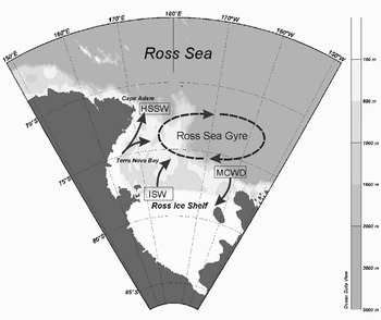
Fig. 1 Large-scale map of the Ross Sea and TNB location. Arrows depict a simplified scheme of the circulation.
The most important feature of TNB is a persistent coastal polynya. The strong katabatic winds blowing offshore form the wind-driven flaw polynya as they advect the newly-formed ice far from the coast (Bromwich & Kurtz Reference Bromwich and Kurtz1984). In the polynya, the low sea-ice concentration results in an intense heat exchange between the cold atmosphere and relatively warm ocean that facilitates frazil ice production and brine rejection. The TNB polynya has an estimated mean size of about 1300 km2 but can reach up to 5000 km2 (Kurtz & Bromwich Reference Kurtz and Bromwich1985) and an annual mean ice production of about 50 km3, as recently derived from Special Sensor Microwave Imager (SSM/I) data and heat fluxes by Martin et al. (Reference Martin, Drucker and Kwok2007). Polynya size, as well as the amount and properties of the High Salinity Shelf Water (HSSW) formed in this area during the winter are strongly controlled by the atmospheric forcing (Gallée Reference Gallée1997, Van Woert Reference Van Woert1999, Assmann & Timmermann Reference Assmann and Timmermann2005, Petrelli et al. Reference Petrelli, Bindoff and Bergamasco2008) and therefore have high interannual variability. In spite of its relatively small size with respect to the Ross Sea polynya, HSSW contribution can be up to 10% of the Ross Sea Bottom Water (RSBW, Kurtz & Bromwich Reference Kurtz and Bromwich1985, Van Woert Reference Van Woert1999). RSBW is a significant part of the Antarctic Bottom Water and plays a crucial role in the deep ocean ventilation (Jacobs Reference Jacobs2004).
Previous studies (Jacobs et al. Reference Jacobs, Amos and Bruchhausen1970, Reference Jacobs, Fairbanks and Horibe1985, Carmack Reference Carmack1977, Locarnini Reference Locarnini1994) identified the Ross Gyre as the feature characterizing the Ross Sea Shelf circulation. The Ross Gyre is formed by a branch of the Circumpolar Deep Water which enters the eastern sector of the region near the shelf break. Water masses circulating westward in the Ross Sea Shelf are modified by air-sea interaction, by mixing with resident waters, and by interaction beneath the Ross Ice Shelf and leave the area colder and denser than when they entered the region. Based upon their origin and characteristics, different water masses have been identified in the Ross Sea Shelf and their names and definitions have evolved over time.
High Salinity Shelf Water, produced in TNB and characterized by temperature close to the surface freezing point and salinity > 34.7 psu, is the densest water mass found in Antarctica (Orsi & Wiederwohl Reference Orsi and Wiederwohl2009). It occupies the bottom layers and fills the deep pit in the central area. The so-called Terra Nova Bay Ice Shelf Water (TISW) is the result of the basal melting of the Drygalski Ice Tongue and characterized by temperature below the surface freezing point and salinity < 34.7 psu. Terra Nova Bay Ice Shelf Water can be found at the intermediate level and in the coastal area. Waters circulating in the surface layer are part of the Antarctic Surface Water (defined by temperature higher than -1.2°C and salinity < 34.5 psu), which mixes in the western part of the Ross Sea with denser resident waters. They undergo a strong seasonal variability due to the sea ice formation and melting processes, being fresher and warmer during summer (Budillon & Spezie Reference Budillon and Spezie2000) than other seasons.
Terra Nova Bay circulation is part of the large scale circulation of the Ross Sea (Fig. 1) and can be roughly represented as a clockwise coastal current (Commodari & Pierini Reference Commodari and Pierini1999). Water masses coming from the western sector of the Ross Sea Shelf circulate in TNB where they are strongly modified by air-sea-ice interactions in the polynya. Water leaves the area flowing north towards Cape Adare and east towards the shelf break region.
Long-term current meter measurements in the Ross Sea were performed in 1978 and 1983 and reported by Pillsbury & Jacobs (Reference Pillsbury and Jacobs1985) who analysed the seasonal variability of the currents in front of the Ross Ice Shelf. Starting in 1994, several moorings were deployed in the western area in the framework of the Italian National Program for Antarctic Research (PNRA), Climatic Long-term Interaction for the mass balance in Antarctica (CLIMA) Project (Spezie & Manzella Reference Spezie and Manzella1999) and US Antarctic Slope (AnSlope) experiment (Gordon et al. Reference Gordon, Padman and Bergamasco2009). Among them, mooring D1, equipped with temperature and salinity sensors, current meters and sedimentary traps, was deployed in the middle of TNB and it is still operating (PNRA 1995).
The time series shows currents in TNB mainly directed north-eastward along the coast, with a small vertical shear and high seasonal and inter-annual intensity variability (Manzella et al. Reference Manzella, Meloni and Picco1999, Picco unpublished). Current observations together with model results indicate that dense water formation processes occur in deeper layers and are able to induce an important thermohaline circulation (Buffoni et al. Reference Buffoni, Cappelletti and Picco2002) even at great depths.
Despite several programmes carried out in the area, and the existence of long-term time series of observation and data from oceanographic campaigns, winter oceanographic observation in the upper thermocline are scarce. One year of Acoustic Doppler Current Profiler (ADCP) data acquired in TNB during 2000 in the upper 160 m of the water column provides the opportunity to have an insight into the upper layer dynamics even during winter. The aim of the present work is to present unpublished ADCP data and to investigate the relative role of surface forcing, such as wind stress and ice melting and formation, in modifying the surface circulation.
Data
Meteorological and sea-ice concentration data
Meteorological observations were obtained from the Automatic Weather Station ENEIDE (AWS 7353, http://www.climantartide.it; accessed September 2005), which is the closest to the coast (74°42′S, 164°6′E) and at about four miles from the mooring. The AWS measures hourly wind speed and direction, air temperature, atmospheric pressure and relative humidity. Wind data from 24 September–19 October 2000 were missing. Daily mean time series of wind speed and direction and air temperature were used in this study.
Sea-ice concentration is available from the Nimbus-7 Scanning Multichannel Microwave Radiometer (SMMR) and Defence Meteorological Satellite Program (DMPS, USA) SSM/I passive microwave analysis archived at the National Snow and Ice Data Center (Cavalieri et al. Reference Cavalieri, Parkinson, Gloersen and Zwally2008). Daily sea-ice concentration, from 5 February 2000–16 January 2001, at 25 km resolution was extracted in a region bounded by 164°E and 165.5°E longitude and 74.5°S and 75.5°S latitude. As shown in Fig. 2, six grid points were within the selected area and used for the analysis.
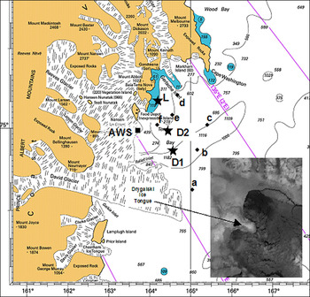
Fig. 2 TNB with location of moorings (stars), Antarctic Weather Station ENEIDE (square) and ice-concentration SSM/I data grid points (dots) used in the analysis. Dark grey areas in the sea map indicate 200 m isobath. In the panel, is a satellite image of TNB polynya on 29 September 2000 from ATSR-2 (Along Track Scanning Radiometer) provided by Rutherford Appleton Laboratory. The dark area north of the Drygalski Ice Tongue highlights the ice-free polynya.
Oceanographic data
Oceanographic data were collected in the framework of PNRA-CLIMA project activities (PNRA 2001). Three fixed moorings (D1, D2, L) deployed in TNB (Fig. 2) provided measurements of currents, temperature and salinity. Mooring D1 has been operating since 1994 for long-term observation in TNB polynya. Mooring L was added in 1999 to monitor coastal waters in the TNB protected area close to the Italian Antarctic Base. Mooring D2, devoted to ADCP measurements, was active from 5 February 2000–16 January 2001 (see Table I for locations of moorings and characteristics). During summer oceanographic campaigns, moorings were regularly recovered for maintenance and data downloading, and then re-deployed. Even if sensors could not be calibrated onboard, temperature and salinity data were compared to the conductivity, temperature and depth measurements performed close to the moorings and corrected for drift and offset. SBE SeaCat sensors installed on mooring D1 had a nominal accuracy of 0.002°C for temperature and 0.003 mS cm-1 for conductivity, stability was respectively 0.002°C and 0.003 mS cm-1 per month. Long-term use in extreme environmental conditions without in-house calibration and maintenance might lower the quality of the measurements.
Table I Mooring positions and payload.

Daily means of currents, temperature and salinity were also obtained from the acquired data. In order to take into account the vector characteristic of horizontal velocity, data analysis was carried out in complex form (east–west component as the real part).
Acoustic Doppler Current Profiler data
The upward-looking, 30° beam angle, 150 kHz narrow-band ADCP was located at a nominal depth of 178 m and sampled the water column up to the surface. Vertical resolution of measurements was 16 m; time interval was one hour and each sample was the average of 60 pings. The nominal standard deviation on the horizontal currents for this setup was 0.56 cm s-1. Data were corrected for the local magnetic declination. Due to the lack of any pressure gauge, the vertical position of the mooring line was deduced from pitch and roll data. The mooring was near vertical during the period of measurements as pitch and roll never exceeded 5°, corresponding to vertical displacements lower than the bin size (16 m). The echo intensity strength mean profile (Fig. 3) resembled the one reported by Shcherbina et al. (Reference Shcherbina, Rudnick and Talley2005) for polar waters and proved that the presence of scatters in the water was enough to ensure a good performance of the instrument. The low concentration of scatters in the clear Antarctic waters could hamper the proper use of lower-frequency ADCP, as occurred during the period 2001–02 to the 75 kHz ADCP installed on the same mooring. An increase of echo intensity was observed in the deeper layers starting from December. Approaching the surface, the signal was characterized by increasing variability, but no seasonal trend was visible. An increase of the echo intensity due to a phytoplankton bloom was detected under similar conditions during long-term ADCP measurements in the Adélie Sill in East Antarctica (Williams et al. Reference Williams, Bindoff, Marsland and Rintoul2008). The maximum signal strength in the upper bin indicated that the ADCP data reached, or even scattered off, the sea surface. Knowing that a strong interface may affect the ADCP measurements, data from this bin were not used. On average, the percentage of good data (at least three of the four beams working correctly) was higher than 95% at all levels (Fig. 3).

Fig. 3 Mean profiles of percentage of good data (left) and ADCP echo amplitude in dB (right).
Horizontal current data were also compared to eulerian current measurements from an Aanderaa RCM7 current meter onboard the same mooring at 89 m depth. Data from the two sets showed good agreement despite a few degrees shift in direction. The shift was probably due to the lack of heading correction of the Aanderaa. Complex correlation analysis according to Kundu (Reference Kundu1976) gave modulus 0.97 and angle 13°.
Automatic Weather Station and sea-ice concentration record in TNB
The wind regime in the area is characterized by katabatic winds that originate on the Antarctic plateau and are funneled towards the sea through the David, Priestley and Reeves glacier valleys. This last is considered the source of the strong, persistent wind responsible for the east–South-east sea-ice drift (Davolio & Buzzi Reference Davolio and Buzzi2002, Petrelli et al. Reference Petrelli, Bindoff and Bergamasco2008). The wind plays an important role in the polynya extension, advecting newly formed sea ice away from the coast. During the acquisition period, excluding low-intensity winds (< 5 m s-1), which were spread over the whole wind rose (Fig. 4), wind directions were concentrated in the western sector and had a mean of 277°N. The mean intensity was 12.6 m s-1 with hourly peaks up to 75 m s-1 (Fig. 5) and standard deviation of 13.4 m s-1. The highest intensities were recorded between late July and the end of August with a maximum daily mean value of 47 m s-1 registered between 31 July and 2 August.

Fig. 4 Wind scatter plot of daily mean data.

Fig. 5 Time series of daily mean data of wind speed and air temperature from AWS ENEIDE; SSM/I ice concentration daily mean data spatially averaged over the six grid points.
Air temperature time series (Fig. 5) followed a typical seasonal cycle: from late November to early February daily mean temperature ranged between -5°C and 0°C and during the long winter (the polar night in the area is from May to early August) mean temperature was -21°C with minima below -30°C. Unlike the summer period, winter temperature had a high variability characterized by warming events with increases up to 20 degrees in a few days. Most warming events were associated with strong winds, as might be expected for katabatic winds (Renfrew & Anderson Reference Renfrew and Anderson2002). The mean temperature over the entire period of record was -14.9°C.
Time series of spatially averaged ice concentration data (Fig. 5) showed a high variability, in agreement with polynya dynamics. Until mid February the TNB region was ice-free, at the end of the month it reached 30% of ice concentration, then rapidly increased, keeping a mean of about 65% from March to October. Ice concentration higher than 80% occurred for short periods, but values above 92% were never reached. According to the criteria proposed by Liu et al. (Reference Liu, Martin and Kwok1997), values between 30% and 80% define a region of frazil ice called “active polynya”. Consolidated thin ice forms when ice concentration is above 80%. For the six grid points in our study area (see Fig. 2), the seasonal evolution was similar, indicating that all of them were in the polynya. Nevertheless, some spatial variability was observed. Lower values were found close to Drygalsky Ice Tongue (grid point a), which prevents the sea-ice advection from the south. Higher ice concentration was observed at grid point c, which is the furthest from the coast and the closest to the polynya boundary. Ice formation started earlier in grid points b and c, in accordance with the general ice formation process in the Ross Sea (Comiso et al. Reference Comiso, Maynard, Smith and Sullivan1990) which is known to start in the south-eastern part and advance north-westward from the shelf.
Time series of temperature and salinity
Daily means time series of temperature and salinity from mooring L and D1 at a depth of 114 and 126 m (Fig. 6) show that the seasonal evolution due to ice melting and formation affected the water column properties also at these depths. In particular, in the coastal area (mooring L), sea ice melting and fresh water from land contributed to lower the salinity to 34.35 psu, while continuous winter ice formation in the polynya increased the salinity to 34.75 psu. As a consequence, offshore density gradient (up 0.25 kg m-3) developed from February–April. Between mid March and October, temperature remained close to the minimum (-1.96°C for mooring L and -1.92°C for D1). These values were just a few hundredths of a degree above the freezing point, which for salinities between 34.6 and 34.75 psu goes from -1.995 to -1.986°C. The almost constant 0.04°C difference between the two time series during winter could be explained in terms of water mass distribution, in particular ice shelf water. We could not however exclude an offset between the two sensors. Salinity increased until October in mooring D1, and then smoothly decreased.

Fig. 6 Time series of daily mean temperature and salinity data from mooring L at 114 m depth (thick line) and from mooring D1 at 126 m depth (dotted line).
From June to September, HSSW formation events lasting a few hours were detected in both 126 m and 526 m 30 min time series (Fig. 7). The two series were highly correlated (correlation coefficient 0.89) and the timing and magnitude of the salinity peaks reflected the vertical mixing occurring in the measurement area.

Fig. 7 30 min time series of salinity at 126 m and 526 m from mooring D1 from 15 June–15 October 2000. Peaks highlight events of HSSW formation.
High Salinity Shelf Water produced in TNB was saltier and denser than that formed in the coastal polynyas in East Antarctica (Williams et al. Reference Williams, Bindoff, Marsland and Rintoul2008), but the salinity and density temporal trend between the formation and peak period was smooth.
Time series of ADCP currents
Currents statistics
Table II reports ADCP current east–west, south–north and vertical (positive upward) components averaged over the whole acquisition period (5 February 2000–16 January 2001) with standard deviations, mean speeds and directions. Figure 8 displays stick diagrams of current vectors highlighting that the circulation was quite active throughout the period examined here. Near-surface horizontal currents were mainly eastward with daily means up to 70.2 cm s-1 and hourly values reaching 150 cm s-1. Mesoscale variability and persistent meandering were also relevant features. Higher surface velocities observed in winter indicate that the sea surface was not ice covered, thus confirming that the mooring was located in the polynya area, as originally planned. Nevertheless, the kinetic energy time series (Fig. 9) show events, such as the one of 15–29 May, when near surface layer currents dropped down to zero, probably because of sea-ice formation. It is well known that ADCP measurements are sensitive to the presence of sea ice, so that some authors suggested an alternative use of ADCP, mainly based on the analysis of echo intensity, for sea-ice draft and coverage estimation (Visbeck & Fisher Reference Visbeck and Fisher1995, Shcherbina et al. Reference Shcherbina, Rudnick and Talley2005, Hyatt et al. Reference Hyatt, Visbeck, Beardsley and Owens2008). The dropping current events were associated with lower wind speeds, low air temperature and an increase in sea-ice concentration. Usually, the absence of winds inhibits the offshore ice transport and allows the consolidation of the frazil ice, confirming the important role of katabatic winds in the control of the polynya size (Gallée Reference Gallée1997).
Table II ADCP currents at each level averaged over the whole acquisition period (5 February 2000–16 January 2001).

Vx = E–W component, Vy = S–N component, Vz = vertical (positive upward) component, SD = standard deviation

Fig. 8 ADCP horizontal currents stick diagrams. Layer 1 at the top of figure.

Fig. 9 Daily mean data of wind (top) and currents kinetic energy in the top two and bottom two levels.
Water below the near surface layer was vertically homogeneous. The water moved to the north-east, in accordance with the bathymetry and the general circulation of Ross Sea. The mean velocity decreased with depth from 40 to 28 cm s-1, an effect also seen in the daily mean kinetic energy time series (Fig. 9).
Complex correlation analysis supports our conclusions regarding different dynamics in the near surface, relative to deeper water. The resulting values were low for the first layer (modulus ranging from 0.4–0.70, angle up to 24°) and increased for the deeper layers (modulus from 0.73–0.98, angle below 7°). Horizontal current seasonality (Fig. 10) could be described by two main patterns: during February–April the transport was south-eastwards and characterized by a great variability and mean velocities of about 20 cm s-1; while from June–December currents were more intense (mean velocity about 30 cm s-1) and presented a more stable north-eastward flow. Eulerian currents observations in deeper layers (500–1000 m) from mooring D1 (not shown here) also depicted a well-correlated system moving north-west along the coast at a mean velocity of about 12 cm s-1 and with a higher variability from June–September.

Fig. 10 Depth-integrated monthly mean currents vectors. Circles represent the estimated error associated with the mean. On the right the dashed vectors are the mean of the two periods (February–April and May–January) and the dash-dot vector is the southern drift.
Vertical velocities (Fig. 11) were in general quite high but attenuated with depth. Peak velocities reaching 20 cm s-1 are visible in the upper layer. The direction was mainly downward, but during the summer the upward component in the two uppermost layers strongly increased. Higher intensity and variability occurred during HSSW formation period (July–September) also in the deep layers, while during the summer vertical velocity was confined to the two upper layers.

Fig. 11 Hourly data of vertical currents at each level.
Empirical Orthogonal Function (EOF) analysis of vertical profile time series
The 16 m vertical resolution of ADCP measurements allowed EOF decomposition of the velocity profile time series. The complex EOF modal decomposition was performed on daily mean horizontal currents with the aim to isolate the main features of the circulation. The first three modes accounted for 76, 20 and 3% of the signal respectively and the imaginary component resulted negligible, indicating a non-rotating structure. The first mode profile (Fig. 12a) was almost uniform in depth, while the second one was characterized by a strong surface shear. The third mode had such a small contribution that it was not included in the analysis. The first mode coefficient temporal evolution (Fig. 12b) displayed higher values from mid June–November, while the second mode coefficient didn’t show a clear seasonal trend. This suggested that the strong wintertime mixing reduced the vertical shear.

Fig. 12 First second and third EOF modes of daily mean horizontal currents, a. real component profiles, and b. temporal evolution of the absolute values of the coefficients.
Figure 13 shows the progressive vectors obtained by separately reconstructing currents described by the first and second mode using mode profiles and time evolution coefficients. First mode currents represented the large-scale barotropic circulation with intensity values attenuating from 40.1 cm s-1 in the surface layer to 26.6 cm s-1 at 160 m. Currents described by the second mode were significant in the surface layer and comparable with those of the first mode. They had a mean intensity of 43 cm s-1 and direction of 110°N. In the lower layers current intensity decreased to a mean value between 6 and 8.5 cm s-1.

Fig. 13 Daily mean horizontal currents EOF modes, progressive vectors of a. first, and b. second mode.
Rotary spectral analysis
Rotary spectral analysis (Gonella Reference Gonella1972) was applied to horizontal currents at each level. The hourly time series were divided into 15 subsamples each 512 hours long. The subsamples were linearly detrended and smoothed before applying Fast Fourier Transform analysis, after which the results were averaged to obtain a mean spectrum for each level. Figure 14 shows a peak in the diurnal tide frequency (0.042 cph) prevailing at every depth both in the clockwise and anticlockwise spectrum. The peak on the semidiurnal band, which accounts for both tide and inertial currents (inertial period is 12.4 h at this latitude), was not well resolved and it has been necessary to apply a high-pass filter (e.g. derivative) to distinguish between the two contributions. In the anticlockwise spectrum, at every depth, energy was also spread in a large band centred on 0.012 cph. Relevant differences were observed between spectra from the different samples, the diurnal tide being the only persistent feature (Johnson & Van Woert Reference Johnson and van Woert2006). Vertical velocity spectra also had the main peak at 24 h and the secondary one at 12 h.

Fig. 14 Rotary mean spectra on 15 samples, 512 hours long, at 16 m and 64 m depth. Dotted lines indicate anticlockwise spectra.
Discussion
One year of oceanographic and meteorological observations in TNB provided an insight into the upper-layer circulation of the area and its variability in response to surface forcing. In general, the presence of a persistent wind-driven polynya makes this area peculiar with respect to the surrounding regions, as the intense air-sea interaction affects surface water characteristics and circulation also during winter. Mean horizontal currents during the measurement period were quite high, well correlated, mainly directed north-east with respect to the general circulation of the area and consistent with previous measurements (Manzella et al. Reference Manzella, Meloni and Picco1999, Picco unpublished). However, the analysis of the temporal evolution of the currents revealed different spatial and time-scale variability in response to the local forcing. In particular, the melting and ice-formation processes and wind stress were the main forcing responsible for the observed variability.
At the end of melting season, from February–April, the difference between the densities measured by mooring L and D1 reached a maximum and the mean current direction showed a southward shift. To estimate the order of magnitude of currents that could be induced by this density gradient, the thermal wind equation was integrated (Gill Reference Gill1982) from the sea surface to a depth H, obtaining Δv ≈ gHΔρ/(ρ0fΔx), where Δv is the southward shift, Δρ and Δx are the difference in density and the eastward distance between the two moorings respectively, ρ0 is a reference density, f the Coriolis parameter and g the gravity. Assuming H = 100 m, Δρ = 0.2 kg m-3, Δx = 15 km, f = 1.4 10-4 s-1 and Δv = 10 cm s-1 geostrophic current was obtained, consistent with the observed southward shift during February–April (Fig. 10).
Results from numerical simulations (Assmann et al. Reference Assmann, Hellmer and Beckmann2003) support the importance of the thermohaline-driven horizontal circulation on the Ross Sea Shelf. In general, an intensification of currents during winter seems to be a typical feature in the Ross Sea region. This is also reported by Pillsbury & Jacobs (Reference Pillsbury and Jacobs1985) who observed more energetic currents from July–September in current meter time series in front of the Ross Ice Shelf.
Continuous ice formation occurring in the polynya enhanced the salinity creating a stronger seasonal cycle with respect to the other ice-covered areas. Dense water formation occurring during July–September and detected by peaks in salinity showed up also in the currents: meandering and rotations, typical of the convective processes, modified the mean constant north-eastward flow, while vertical velocities were stronger and displayed higher variability. Contrary to the surface forcing, dense water formation was able to affect the water column up to greater depth. A correlation between winter increases of salinity and horizontal current kinetic energy in deeper layers was also observed over several years of measurements in TNB (Picco unpublished) and has been explained in terms of the thermohaline forcing (Buffoni et al. Reference Buffoni, Cappelletti and Picco2002).
Complex EOF decomposition analysis was an efficient method to separate the contribution of the large-scale vertically homogenous circulation from the wind driven circulation. The second EOF mode (Fig. 13b) described a net offshore transport in the upper layer, in good agreement with the prevailing wind direction; complex correlation coefficient modulus and angle being 0.5 and 18° respectively.
A steady Ekman model (Pedlosky Reference Pedlosky1979) has been applied to estimate the effects of wind on surface circulation. The equations were numerically integrated (vertical resolution 2 m, time step 2 min) over a surface layer of 200 m depth using the slip condition at the bottom layer, a constant value (0.01 m2 s-1) for turbulent viscosity (Timmermann & Beckmann Reference Timmermann and Beckmann1999) and time independent wind stress. Daily mean wind stress was computed from AWS Eneide wind data according to the Hellermann & Rosenstein (Reference Hellermann and Rosenstein1983) formula for the neutral drag coefficient and excluding wind intensities below 4 m s-1 (Large & Pond Reference Large and Pond1981). The computed 32 cm s-1 Ekman current, averaged over the upper 16 m, is comparable to the second mode EOF decomposition reported here. A Coriolis parameter of 1.4 10-4 s-1 yields an Ekman depth of 11.8 m, which could be considered in good agreement with the second mode profile, despite the 16 m ADCP vertical resolution. Numerical results from wind driven circulation models in the western Ross Sea (Bergamasco & Carniel Reference Bergamasco and Carniel2000) assess that the wind stress acts as a relevant forcing for the surface large scale circulation in TNB, but has negligible effects on the vertically-integrated transport (Commodari & Pierini Reference Commodari and Pierini1999).
Acknowledgements
The Italian National Program of Antarctic Research (PNRA), Technologies 2003/11.4, supported this work. Data analysed were collected in the framework of PNRA-CLIMA Project. Thanks are due to Stefania Furia from ENEA CRAM for help with drawing the figures. The constructive comments of the reviewers are also gratefully acknowledged.


