Introduction
During summer, meltwater ponds are common features in many ice-free parts of Antarctica, where they typically represent isolated foci of biological activity and diversity in otherwise barren, desert landscapes (Vincent & James Reference Vincent and James1996, Howard-Williams & Hawes Reference Howard-Williams and Hawes2007, Quesada et al. Reference Quesada, Fernández-Valiente, Hawes and Howard-Williams2008). These are often closed-basin ponds, lying in shallow depressions and may be long-lived phenomena. Water lost by evaporation, ablation and sublimation is replenished by melting of winter snow and/or glacial ice. During summer, water is maintained in the liquid state by relatively mild air temperatures and the absorption of incident solar radiation within the pond/sediment system (Hawes et al. Reference Hawes, Howard-Williams and Pridmore1993, Reference Hawes, Schwarz, Smith and Howard-Williams1999). When melted, growth conditions in these ponds can be rather benign, with water temperature reaching up to 10°C. The biotic assemblages in these ponds are dominated by species-rich, perennial mats of algae and cyanobacteria that can grow to centimetre thickness and cover the entire benthic area. Photosynthesis by these microbial mats can reduce nutrients and inorganic carbon to extremely low concentrations and drive pH to values of over 10 (see reviews by Howard-Williams & Hawes Reference Howard-Williams and Hawes2007, Hawes et al. Reference Hawes, Howard-Williams and Fountain2008 and references therein).
A paradox of our understanding of polar ponds is that most studies occur during this relatively benign period when researchers can most easily access them, while the most extreme stresses are likely to occur during and after the process of freezing. Previously (Hawes et al. Reference Hawes, Schwarz, Smith and Howard-Williams1999), based on over-winter data logging, experimental manipulations and limited direct observations (e.g. Schmidt et al. 1991), we have speculated on how the environmental changes that must accompany pond freezing may affect the microbial communities that dominate these ponds. We postulated that the extreme autumn and winter conditions were more likely to impose the uniquely “Antarctic” characteristics of these systems than the relatively mild summer conditions. In January 2008, a unique opportunity to observe the freezing process arose when the United States and New Zealand Antarctic Programmes combined to extend field science support in the McMurdo Sound region from January through until April. This allowed us to access ponds on the McMurdo Ice Shelf for much of the freezing period and to obtain detailed records of physical, chemical and biological change. This contribution sets the scene for a series of reports on the freezing process by describing physical conditions during freeze-up.
Study area
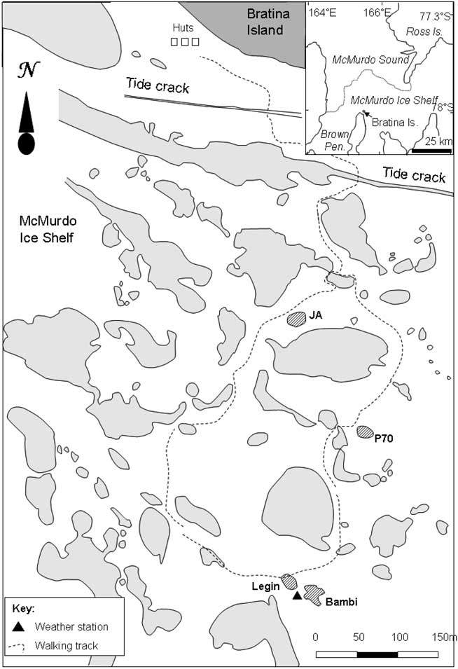
The McMurdo Ice Shelf (MIS) is a small part of the Ross Ice Shelf, located in the south-west corner of the Ross Sea (Fig. 1). It is bounded by Minna Bluff to the south and the coast of southern Victoria Land to the west. On the eastern side, the MIS grades into the Ross Ice Shelf proper, while to the north it meets the episodically ice-free waters of the McMurdo Sound. The MIS is one of the most extensive surface ablation areas in Antarctica (Swithinbank Reference Swithinbank1970), yet it does not ablate entirely due to a unique characteristic of the area - nourishment of the floating ice shelf by the freezing of seawater beneath (Debenham Reference Debenham1920). As a consequence of this mechanism, there are large amounts of debris on the surface of the MIS. This debris is marine sediment that is incorporated into the ice during basal freezing, which then slowly migrates to the ice surface as the surface ice ablates, at rates of approximately 0.5 m yr-1 (Gow & Epstein Reference Gow and Epstein1972). The density of debris varies, giving rise to two types of ice surface topography, the “pinnacle ice” and the “undulating ice” (Howard-Williams et al. Reference Howard-Williams, Pridmore, Downes and Vincent1989). Pinnacle ice is highly dynamic, with thin patches of sediment, ephemeral meltwater channels and pools forming amongst ice mounds with a relief of 1–2 m. Undulating ice is, by contrast, slow moving and stable. It occurs primarily between Bratina Island and Brown Peninsula, has a rolling surface relief of approximately 10 m, with most of the surface covered by > 100 mm of sediment. The terrain comprises an array of sediment-lined, long-lived meltwater ponds of a few 10s to 100s of square metres, lying between rounded mounds of ice-cored sediment. In this study we focus on four of the smaller ponds on the undulating ice, Legin, Bambi, P70 and JA (all unofficial names), selected for their broadly similar size, shape and bathymetry (Table I). We assessed that their size was sufficiently large to accommodate planned water sampling with no significant loss of volume but small enough for samples to be volumetrically representative. All were within walking distance of a field laboratory at Bratina Island.

Fig. 1 Location map of study area, to the south of Bratina Island on the McMurdo Ice Shelf. Ponds are shown in grey, with the main study ponds hatched.
Table I Physical properties of the four ponds used in this investigation.
Note: all names are unofficial
Methods
Meteorological variables
Weather conditions for the duration of the study (27 January–8 April 2008) were recorded using a CR10X (Campbell Scientific) datalogger linked to appropriate sensors. Incident radiation was obtained using a LiCor pyranometer and air temperature using a Vaisala combination temperature/humidity sensor. From 27 February onwards, Campbell Scientific 107 temperature sensors were installed at 20, 60 and 155 cm depth in Legin. These were allowed to freeze into holes drilled in the ice, which filled with underlying pond water. All sensors were interrogated by the datalogger at 60 second intervals and an hourly mean recorded. A daily mean was calculated for irradiance.
Sampling
The study period began in late January, shortly before ice formed, and continued through to 7 April 2008. With respect to sampling methods, two periods can be identified. The first comprised the open water period and that time when ice was formed but was insufficiently thick to walk on. The second began when ice formed a stable sampling platform. During the first period, all sampling was from the shore and measuring devices were extended out into the ponds using a 4 m long telescopic aluminium pole or suspended from a pulley attached to a line that was stretched across the pond between two stakes. Under these conditions the exact sampling point was not reproducible and we could not confidently detect the deepest part of the ponds. Once the ice was secure, on 7 February, sampling was carried out through holes drilled through the ice. From this point onwards, the deepest part of the pond could be located reliably and greater vertical resolution was possible by attaching sampling tubes and instruments to graduated plastic-coated steel rods. The consequences of this change in regime were most significant for Bambi and Legin ponds. Sampling from the edge, we estimated Bambi to be 1.1 and Legin to be 1.2 m deep and both to be well mixed. Once the ice could be used to sample from Bambi was found to be 1.25 m deep and mixed, while Legin was 1.6 m deep and density stratified.
Ice thickness and water depth
Ice thickness and water column depth were determined using a rod. For depth the rod was lowered until it just touched the sediment surface and the depth to the water level in the sampling hole recorded. For ice thickness the rod was drawn up through the water column until a right-angled protrusion on its end just contacted the underside of the ice.
Ice transparency and albedo
Once ice had formed and could be walked on, spectral ice transparency was measured approximately weekly using a spherical irradiance collector (Walz Instruments, http://www.walz.com) mounted on a fibre-optic cable, connected to an Ocean Optics S2000 Spectrometer (http://www.OceanOptics.com) linked to a laptop computer. For each measurement, the spectrometer was first zeroed with the light collecting element in the dark, and then set to 100% in daylight while held over a black cloth to eliminate backscattered radiation. The light collecting element on the fibre-optic cable was then pushed down through a 50 mm hole in the ice. A small float attached to the cable just behind the collecting sphere brought the latter to the underside of the ice; it was pushed out away from the hole for 0.5 m to minimize “hole effects”. At least three replicate scans from 430 to 700 nm wavelength were recorded and interpreted as percentage transmission of the ice (this is not exactly correct as a small amount of irradiance may have been reflected from the pond sediment surface back up to the sensor). The instrumentation could not record at wavelengths shorter than 430 nm.
Albedo of the ice cover was determined using the same apparatus but with an Ocean Optics cosine corrected irradiance collecting head replacing the spherical head. The spectrum of downwelling irradiance was recorded first, then that of the upwelling irradiance 50 mm above the ice surface. Albedo, measured as percentage reflection, was calculated for two types of ice, white ice, which contained high densities of gas bubbles and dominated the study ponds, and black ice, which contained few gas bubbles and occurred on other, larger ponds.
Water column temperature and conductivity
A C-90 conductivity-temperature meter (TPS Ltd, Springwood, Australia) was used to measure temperature and conductivity. The probe was calibrated for conductivity daily using a 2-point procedure against air and a conductivity standard. Temperature calibration was checked weekly at 0°C using an ice-water bath. Data were recorded against depth during downwards profiling but, because of changes in overall pond depth, were subsequently converted to distance from the pond bottom.
Bathymetry and hypsographic curves
Bathymetry of the four ponds was determined just after ice cover had formed. The new ice cover comprised a very flat surface through which a 1 m spaced grid of 15 mm diameter holes was drilled. Water depth at each hole was determined and a bathymetric map produced by interpolation of these data. Contours were drawn at 10 cm depth intervals and the area contained by each contour estimated using the image analysis package “Image-J” (http://rsb.info.nih.gov/ij/). Depth-area and depth-volume plots were constructed and a second or third order polynomial fitted (whichever gave the best fit) using the curve fitting element of Sigmaplot 10 (http://www.sigmaplot.com/). These curves were used to estimate residual water volume or sediment surface area from ice thickness and water depth.
Results
Meteorological conditions
During the study period air temperature fell from just below zero in January to -30°C in April (Fig. 2). Considerable diel and day-to-day variation was evident, with occasional rapid rises in temperature (Fig. 2), always accompanying periods of persistent strong winds from the south. Over the same period, mean daily irradiance incident to the study area fell more than tenfold from approximately 200–250 to 10–20 W m-2. By the end of February midnight irradiance was less than 1 W m-2 and by the end of the study period this condition was met for more than half of each day.
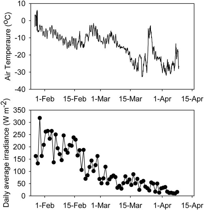
Fig. 2 Air temperature (hourly mean) and irradiance (daily mean) during the sampling period. All variables are sampled at 1 minute intervals.
Ice thickness and water depth
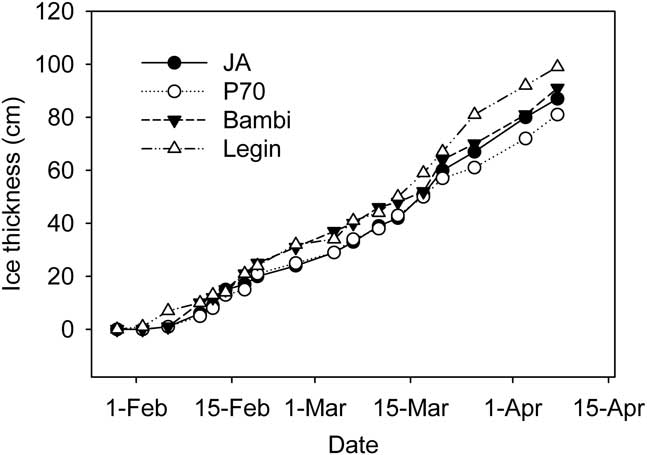
Ice was observed on all of the ponds in late January, though this was thin and ephemeral; persistent ice formed on 2 February 2008. The thickness of ice on the four ponds then increased steadily (Fig. 3), at rates which averaged 1.5–1.6 ± 0.4 cm d-1 for each pond (arithmetic mean of ice growth between measurements ± 95% c.l.). By the end of the study period each pond had 81–92 cm of ice. Because of different starting depths, this left JA virtually dry, while P70 and Bambi had 25 and 40 cm of liquid water remaining and the deepest pond, Legin, still retained 80 cm of liquid water (Fig. 3). We converted water depth to residual unfrozen pond volume and sediment area, expressed as a percent of those at the start, using the polynomial relationships developed between area, volume and depth. In calculating these values we assumed that ice thickness was constant across the pond surface; limited testing of this assumption was supportive. Residual volume and area declined rapidly at first but was slowed in early March and towards the end of the study period (Fig. 4). In all cases, the percentage volume declined more rapidly than percentage area. In the larger Bambi and Legin ponds, 20 and 35% of pond area and 5 and 15% of volume remained unfrozen at the end of the study. In the smaller JA and P70 ponds, little water and only 5–10% of sediment remained unfrozen.

Fig. 3 Ice thickness at fixed locations in four ponds on the McMurdo Ice shelf during the study period.
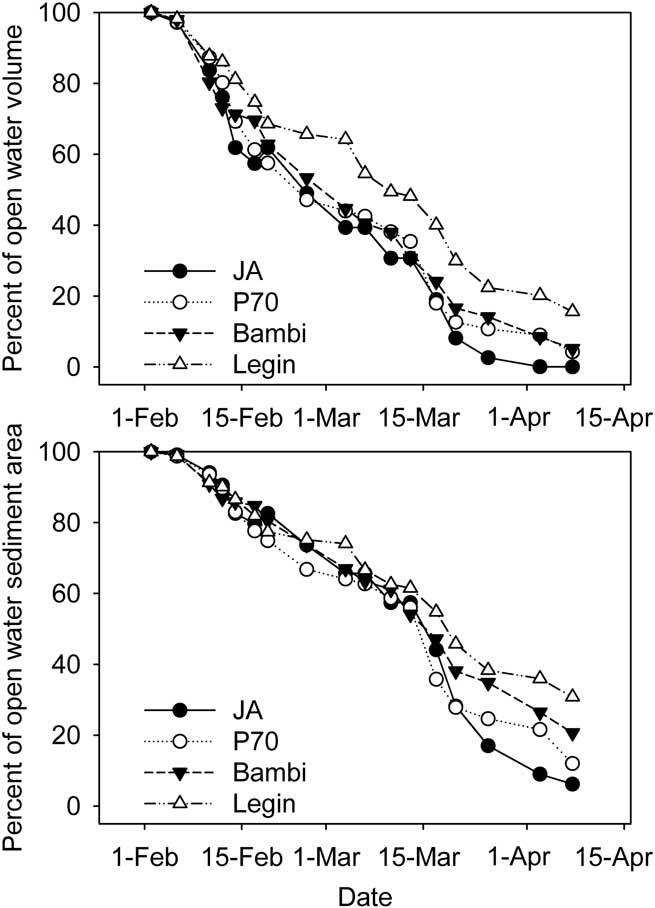
Fig. 4 Residual pond volume and sediment area in four ponds of the McMurdo Ice shelf. Estimates are from hypsographic curves, pond depth and ice thickness.
Ice and water temperature
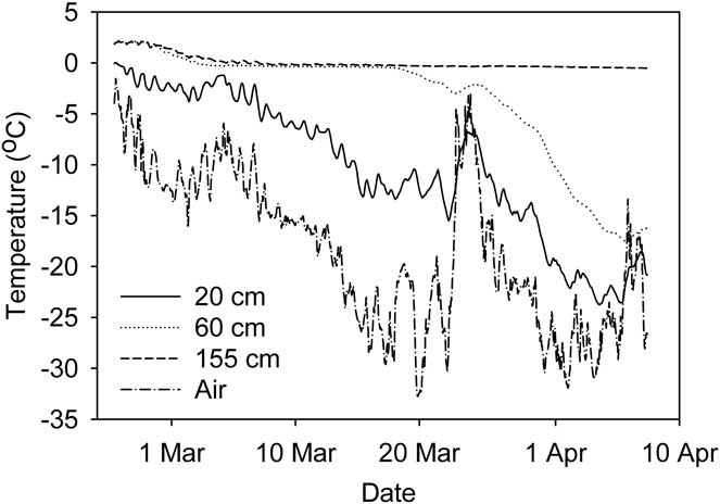
Continuous records of ice and water temperature in Legin from 27 February–7 April showed how the ice front gradually moved through the water column (Fig. 5). Ice temperature at 20 cm typically followed the short-term variability of the air temperature. At 60 and 155 cm depth, water reached the freezing point by early March. At 60 cm the temperature remained at freezing until ice formed two weeks later, while at 155 cm freezing had not occurred by 7 April. Ongoing temperature records (not presented here) show that ice formed at this depth in early May.

Fig. 5 Temperature of ice/water at three depths in Legin pond. Air temperature is also shown. Records are hourly averages.
Ice transparency
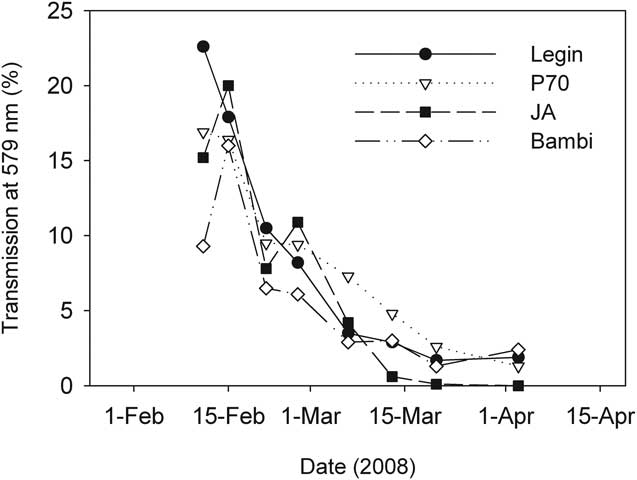
The first ice to form in February was clear and highly transparent, but transmission of irradiance through the ice declined over time as ice became opaque and its thickness increased (Fig. 6). The wavelength of maximum transmission for all four ponds was at 570 nm, though overall, transmission was not strongly spectrally structured. This was consistent with the appearance of the ice which was essentially white, largely due to the inclusion of large numbers of frosted bubbles into the ice matrix.

Fig. 6 Transmission of irradiance through the ice covers of four ponds on the McMurdo Ice Shelf during February–April 2008.
The vertical attenuation of irradiance by pond ice was proportional to ice thickness, and from the data in Figs 3 & 6, Legin pond's ice extinction coefficient for irradiance at 570 nm could be calculated from log-linear regression as 5.3 m-1 (r 2 = 0.96). To obtain this coefficient the datum from 2 April were discarded as an outlier to an otherwise good relationship. In April, under-ice irradiance approached the detection limit of our instrumentation and we believe that this justified exclusion of this data point. Similar log-linear regressions for other ponds all yielded significant extinction coefficients (P < 0.005), with some variability between ponds. JA ice was most opaque at 5.2 m-1, Bambi intermediate at 4.9 m-1, while P70 the clearest at 3.6 m-1.
As expected, the albedo of the bubble-rich white ice that completely covered all study ponds was high, averaging > 50%. This compared to∼10% for bubble-poor black ice at a nearby pond, and demonstrates the importance of gas bubbles in reducing ice transmission. Albedo peaked at a similar wavelength to transmission, 570 nm and, like transmission, was not strongly spectral.
The combination of declining incident irradiance and ice transparency resulted in a fall of more than two orders of magnitude in daily average sub-surface irradiance over the study period, from 225 W m-2 at the beginning of February, to 10 W m-2 at the beginning of March and to < 1 W m-2 at the start of April.
Water column conductivity and temperature
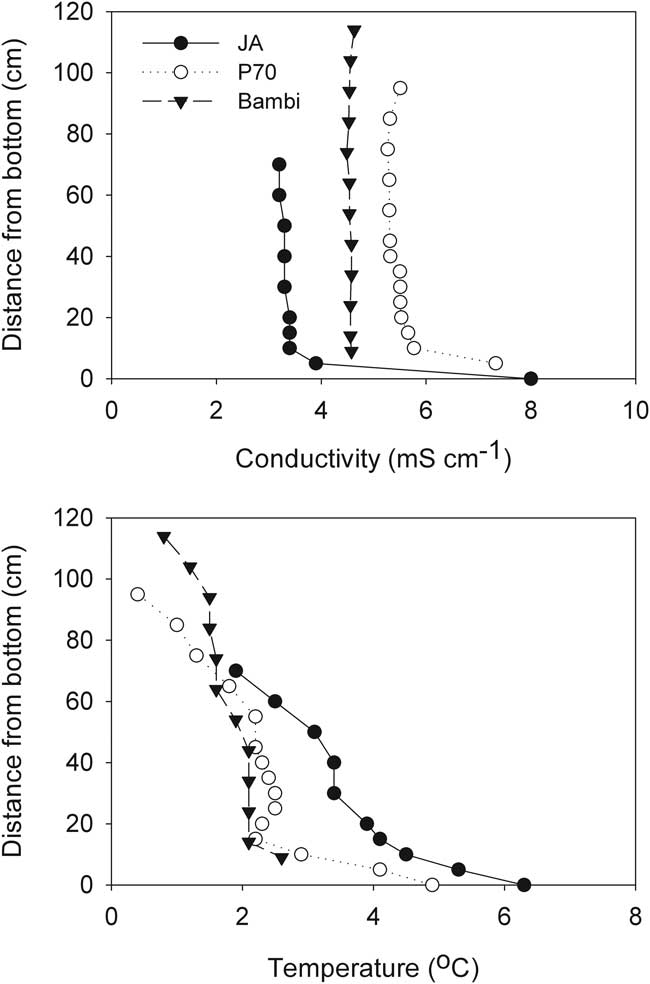
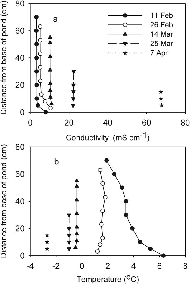
The first profiles of conductivity and temperature after the ice formed showed that JA, P70 and Bambi had little vertical structure to their water columns aside from a slight increase in temperature with depth. Slightly elevated conductivity was evident at the bases of these ponds, with the remainder of the water columns isohaline. Temperature in these three ponds was close to or less than 4°C, allowing the low surface temperature to density-stabilize their inverse temperature profiles (Fig. 7). These weakly stratified ponds all followed a similar trajectory as the freezing process progressed, which resulted in enhancement of vertical homogeneity. Temperatures eventually fell below zero and conductivity increased substantially. Figure 8 shows the process in JA as an example.

Fig. 7 Vertical profiles of specific conductivity and temperature one week after ice formation in three McMurdo Ice Shelf ponds.

Fig. 8 Development of vertical profiles of a. conductivity, and b. temperature during progressive freezing in the mixed JA pond (McMurdo Ice Shelf). Profiles are shorter as the ice thickens.
In contrast, at the start of the freezing process Legin was distinctly stratified by conductivity, which increased from 3 mS cm-1 at the surface to over 40 mS cm-1 at the base (Fig. 9). Deep temperature in Legin exceeded 4°C, but any buoyancy that this warmth might have provided was offset by the increasing conductivity with depth. In Legin, as in the other three ponds, the upper part of the water column remained mixed through the freezing process, although the increasingly concentrated mixed layer gradually entrained the density gradient into the mixed layer (Fig. 9). In addition, in Legin temperature declined rapidly over time in the deeper parts of the density gradient, indicative of heat flow to the sediments of the pond.
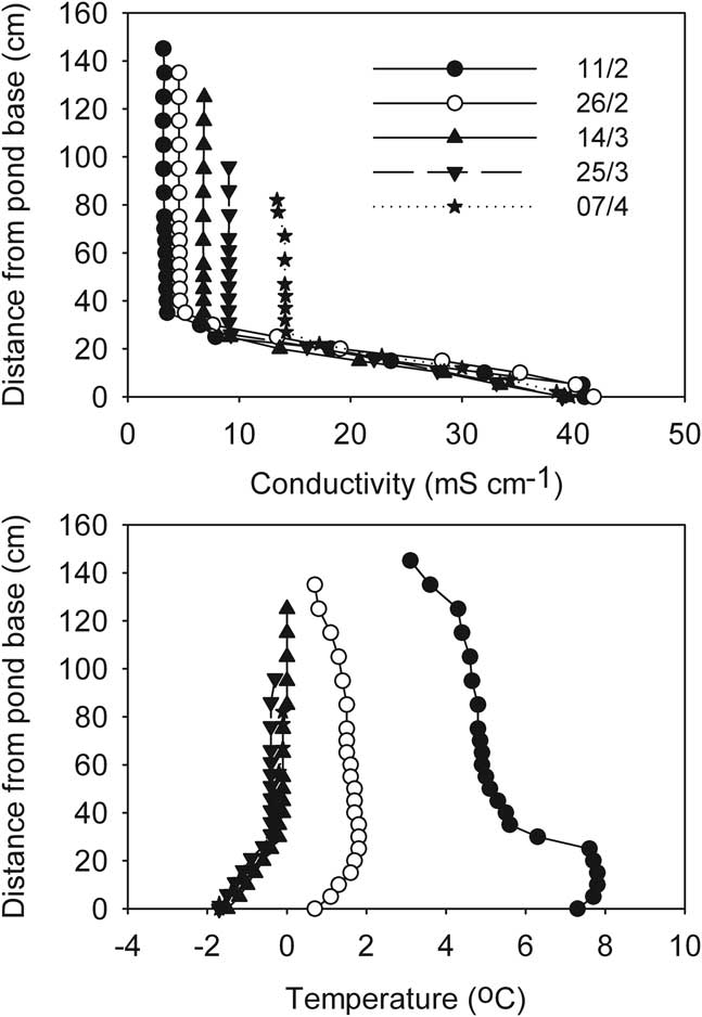
Fig. 9 Development of vertical profiles of a. conductivity, and b. temperature during progressive freezing in the stratified Legin pond (McMurdo Ice Shelf). Profiles are shorter as the ice thickens.
The residual volume of liquid (Fig. 4) was used in conjunction with conductivity to determine the strength of coupling between ice formation and observed conductivity changes. To do this we calculated the product of specific conductivity and volume of residual water - units (mS cm-1)·m3. Gross changes in the product of conductivity and volume over time should be indicative of a shift in the extent to which salt exclusion alone determined residual water conductivity. The most extreme case, that of JA which underwent the greatest proportion of water freezing and reached the highest conductivity, showed a stable conductivity-volume until mid-March, thereafter it declined to a markedly lower value (Fig. 10).
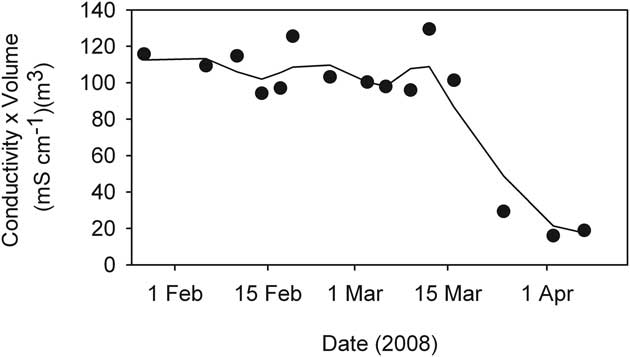
Fig. 10 The product of conductivity and volume during the freezing process in JA pond, (McMurdo Ice Shelf). Symbols mark actual samples while the line is a 3-sample running mean.
Discussion
Aquatic conditions within ponds on the McMurdo Ice Shelf changed rapidly during the two month period following the commencement of ice formation. As ice thickened, irradiance within the ponds declined and water temperature quickly approached freezing temperature as heat was lost both through the ice cover and to the underlying terrain. Exclusion of salts from the ice matrix during the freezing process resulted in a proportional rise in residual water conductivity eventually resulting in extremely high conductivities (> 50 mS cm-1). As ionic content increased, temperature fell below zero as the freezing point of the ever-concentrating brines decreased. In all cases, conductivity/temperature profiles suggested that some form of mixing was keeping the entire water column, or in Legin the upper part of it, well stirred. We suggest that localized density increases at the ice-water interface caused by salt exclusion are the most likely mechanism driving this mixing that was evident in the upper layers of all four ponds. However, it was evident that the simple concentration process driving conductivity eventually broke down (Fig. 10). This can best be explained by sequential precipitation of mirabilite and other minerals as solubility products are exceeded (Wait et al. Reference Wait, Webster-Brown, Brown, Healy and Hawes2006). Nevertheless, cold, dense brines accumulated through this concentration process and these have been postulated to explain the stratification of many Antarctic ponds in the succeeding summer even after ice has melted, despite these ponds being very shallow and having prevalent strong winds that are capable of mixing weakly stratified ponds (Wait et al. Reference Wait, Webster-Brown, Brown, Healy and Hawes2006). Indeed, while Legin was the only pond that was markedly stratified at the start of the study period, all four ponds showed some evidence of a residual brine pool before ice formation began.
The near linear rate of ice formation was unexpected since we had anticipated the insulating effect of ice to slow the rate of freezing over time. Once the bulk of the well-mixed water column reached its freezing point, heat loss was still required at the ice-water interface to remove the latent heat of freezing. The rate of ice formation would have been determined largely by the rate that heat diffused upwards from the ice-water boundary, and perhaps downwards into the underlying sediments. The heat flux away from the interface is dependent on the thermal conductivity and the immediate temperature gradient within the ice. A near constant rate of ice formation requires a near constant temperature gradient, despite increasing ice thickness. Our data allow us to examine this requirement for the water-ice-air connections at the pond surfaces, but not the water/sediment/ice shelf connection at their bases. The ice-water interface can be assumed to be at a temperature of 0°C or just below, thus a constant temperature gradient through the ice requires that air temperature co-vary with ice thickness. Figures 2–5 suggest that this may be the case, as ice and air temperature decrease in parallel with each other and with the increasing ice thickness. Pearson's correlation coefficient of ice thickness on JA and average air temperature for three days prior to the ice measurement (data in Figs 2 & 3) was highly significant at r 2 = -0.767 (n = 16, P = 0.00052).
A second unexpected feature accompanying ice formation was the large number of small gas bubbles that accumulated within the pond ice. This particularly affected the rate of decline in within-pond irradiance and will thus have been a major factor affecting the extent to which photosynthesis could continue in the liquid phase after ice formed. Gas bubbles are frequent inclusions in Antarctic lake ice and result from exclusion of gases from the ice crystal matrix during freezing causing localized gas supersaturation (Adams et al. Reference Adams, Priscu, Fritsen, Smith and Brackman1998). At the end of open water, the mixolimnion of the ponds will have been close to saturation with respect to most atmospheric gases. Exclusion of gases during ice formation will have raised partial pressures of all gases above saturation immediately and the gases in the ice no doubt reflect dissolution. Biological processes may also have played a part in the case of oxygen; as long as whole pond photosynthetic oxygen production exceeded consumption, oxygen mass may have continued to increase within the sealed ponds and further contributed to ebullition. Measurements of irradiance versus photosynthesis in benthic microbial mats from ponds on the McMurdo Ice Shelf suggest that net photosynthetic rate saturates above 100 W m-2, and passes through zero at 25 W m-2 (Hawes et al. Reference Hawes, Schwarz, Smith and Howard-Williams1999). Hawes et al. (Reference Hawes, Safi, Webster-Brown, Sorrell and Arscott2011) show that photosynthesis continued for several days after ice formation, adding to gas supersaturation, but a negative net oxygen flux was evident in late February.
The rate of ice formation is important in determining the duration that microbial communities need to withstand the cold, dim, increasingly saline conditions in the ponds before they enter the fully frozen state. We have shown that the heat gradient through the ice is a key driver of ice formation, thus year-to-year and place-to-place variability in residual liquid water will be climatically controlled. However, similarities in the rates of ice formation across ponds in a single location means that between-pond variability in the residual volume of liquid water and area of unfrozen pond sediments is primarily a function of starting depth. In the case of JA, within one month over 50% of pond volume was frozen and after two months this had reached 99%. In the deepest pond, Legin, after one month 50% of volume had also been frozen, but after two months this had only increased to 90%. However, volume may be less important than sediment area in these ponds, as much of the production and mineralization processes in Antarctic ponds are associated with benthic rather than planktonic communities (Howard-Williams & Hawes Reference Howard-Williams and Hawes2007, Quesada et al. Reference Quesada, Fernández-Valiente, Hawes and Howard-Williams2008). The proportion of the pond floor frozen was consistently lower than that of the water volume. Data presented in Fig. 4 indicates that after one month, 66–81% of the pond floor remained unfrozen in the four ponds while at the beginning of April JA, P70, Bambi and Legin had 9, 21, 27 and 38% of their sediment area remaining clear of ice.
This investigation has described the physical processes that must be tolerated by their biota during autumnal freezing of Antarctic ponds. It is clear that significant areas of pond benthos experienced low temperatures, below-compensation irradiance and elevated salt and gas concentrations under liquid conditions for many weeks before they were frozen. Indeed, over one third of the benthos in Legin was still liquid in mid-April and organisms in that part of the pond are likely to have experienced as much time under liquid and dark as under liquid illuminated conditions. Pond biota will have had to accommodate the combination of a switch from lit to unlit conditions, a near exponential increase in ionic content of pond water over time, and with temperatures decreasing to well below zero.
Overall, when combined with previous studies of the seasonal cycle in these and similar ponds (Schmidt et al. Reference Schmidt, Moskal, De Mora, Howard-Williams and Vincent1991, Hawes et al. Reference Hawes, Schwarz, Smith and Howard-Williams1999) our findings suggest that at 78°S pond organisms experience approximately one month of open water conditions, two of ice covered, near-dark cold but liquid, eight months frozen and one month thawing out. While observations were made on the McMurdo Ice Shelf, we expect the general principles to be broadly applicable to other shallow aquatic systems in Antarctica. In other locations or in years with different weathers, the prevalence of extreme conditions during freezing will vary. Depth has emerged as likely to have biological consequences in Antarctic ponds not just in how it determines summer growth conditions, but also in the duration and distributions of stresses that it imposes during freeze-up. Communities in shallow systems, experiencing low autumnal temperatures, will be frozen before extreme darkness and high conductivity are imposed. Deeper ponds or those with less extreme autumn temperature will increasingly have areas where these stresses are acting on communities before they freeze. Which phases place greatest stress on organisms cannot be determined from this study, but while tolerance of freezing is an obvious pre-requisite for life in Antarctic ponds, it is not the only one.
Acknowledgements
This research was funded by the New Zealand Foundation for Research, Science and Technology (Contracts C01X0708 and C01X0306) to the National Institute of Water and Atmospheric Research (NIWA). Antarctica New Zealand provided logistic support, in collaboration with the US National Science Foundation. Nat Wilson was an integral part of the field team. We are grateful to NIWA Christchurch for laboratory, technical and infrastructural support, particularly to Dr Clive Howard-Williams, and to two anonymous reviewers for critical comments on the manuscript.