


Introduction
The standing biomass and spatiotemporal dynamics of Antarctic krill (Euphausia superba Dana) is a major focus of Antarctic research, with considerable effort focused on modelling rates of krill consumption by Antarctic predators. In 2004, the Commission for the Conservation of Antarctic Marine Living Resources (CCAMLR) tasked a sub-group of the Working Group on Ecosystem Monitoring and Management (WG-EMM) to determine what was currently known about populations of Antarctic krill predators breeding in the Antarctic (Southwell et al. Reference Southwell, Forcada, Goebel, Hinke, Lynch, Lyver, McKinlay, Ratcliffe, Ramm, Reid, Reiss, Trivelpiece, Trivelpiece and Trathan2009). In 2008, a workshop was held in Hobart, Australia with the aim of initiating an effort to: 1) consider procedures for deriving abundance estimates for priority land-based predator species in the south-west Atlantic region between 70°W and 30°W, 2) examine available existing datasets to determine the degree to which minimum data requirements are met, and identify inadequacies or gaps in existing data, and 3) identify and prioritize gaps in existing data as a basis for assessing whether, where and how any future survey work would be conducted. Pursuant to these objectives, a comprehensive database of penguin breeding locations and abundances was created by the task group (Southwell et al. Reference Southwell, Forcada, Goebel, Hinke, Lynch, Lyver, McKinlay, Ratcliffe, Ramm, Reid, Reiss, Trivelpiece, Trivelpiece and Trathan2009). This database contained, for each snow-free coastal area in Food and Agricultural Organization (FAO) Statistical Area 48 either known to host breeding penguins or confirmed as devoid of breeding penguins, the following information: the most current census data (including confirmed absences) and, where appropriate, derived population estimates, along with ancillary information pertaining to the date of last census, the object counted (e.g. occupied nests, adults, etc.), census precision, and the method of census (e.g. count of individuals from the ground etc.). We used this database to identify those locations that contribute most significantly to uncertainty in estimates of the total breeding penguin population for FAO Statistical Area 48, which includes the Antarctic Peninsula and the South Shetland Islands (Subarea 48.1), the South Orkney Islands (Subarea 48.2), South Georgia (Subarea 48.3) and the South Sandwich Islands (Subarea 48.4) (Fig. 1). Area 48 is one area in which the Antarctic krill fishery operates and where there is the greatest potential for resource overlap between the fishery and krill-dependent predators such as penguins. We considered breeding populations of all three species of Pygoscelis penguin (gentoo penguins (Pygoscelis papua Forster), Adélie penguins (P. adeliae (Hombron & Jacquinot)), and chinstrap penguins (P. antarctica Forster)). Macaroni penguins (Eudyptes chrysolophus Brandt) are also important consumers of krill, however, their population in Area 48 occurs largely at South Georgia where the population has been reviewed recently by Trathan et al. (Reference Trathan, Ratcliffe and Masden2012). Elsewhere in Area 48 macaroni penguin colonies are relatively small and so were not considered in our analysis.
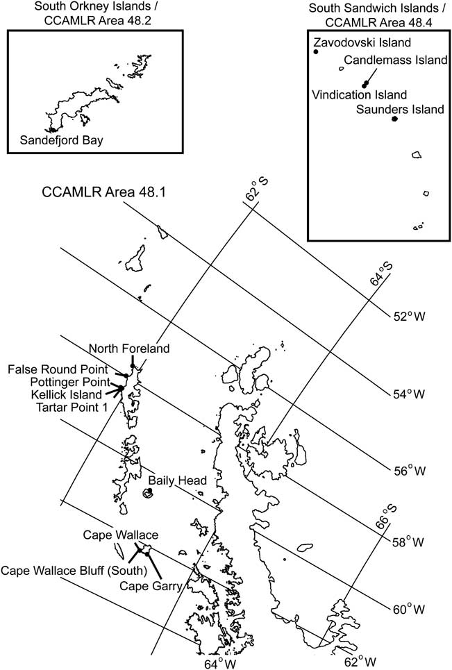
Fig. 1 Study area. Map of the 14 high-influence breeding locations within CCAMLR Area 48. Note that Area 48.3 is not shown.
Methods
Three pieces of information were included for each site in the database: 1) the population estimate (number of breeding pairs), 2) the uncertainty of the census, and 3) the year of the most recent census. Census uncertainty was defined by the commonly adopted and widely accepted five-point scale used by earlier authors (e.g. Croxall & Kirkwood Reference Croxall and Kirkwood1979, Woehler Reference Woehler1993, Naveen & Lynch Reference Naveen and Lynch2011; note that in our analysis the upper bound for N3 has been increased from 15% to 25% to ensure continuity):
N(C)1 Nests (chicks) individually counted, accurate to better than ±5%
N(C)2 Nests (chicks) individually counted, accurate to 5–10%
N(C)3 Accurate estimate of nests (chicks), accurate to 10–25%
N(C)4 Rough estimate of nests (chicks), accurate to 25–50%
N(C)5 Estimate of nests (chicks) to nearest order of magnitude
Our analysis involved a stochastic simulation in which the current penguin population at each site was drawn from a random distribution based on available information. An ensemble of these random draws resulted in a statistical distribution reflecting the accumulation of all pertinent sources of uncertainty. The simulation involved six stages. We illustrate this here using an N2 count of penguins in 1995. Note that for clarity, all stochastically drawn variables are capitalized and given the index i to emphasize that the entire process is repeated to build a distribution that informs us as to the variability in the population estimates. The simulation procedure was as follows:
1. Draw a fractional error for the original census. Using our example of an N2 count in 1995/96, we would draw a number (E i) from the uniform distribution Unif(0.05,0.10) to represent the assumed uncertainty of the original count, i.e.
 $$ {{E}^i} {\rm{\sim }}Unif\,{\rm{(}}{\it 0.05,0.10}{\rm{)}} \eqno\rm$$
2. Draw a count for the true population size (
$$-->$<>C_{{true}}^{i} $$$) at the time of the most recent census (in this case, 1995/96), i.e.$$C_{{true}}^{i} \sim N\left( {{{C}_{original}},{{{\left[ {\frac{{{{E}^i} }}{2}{{C}_{original}}} \right]}}^2} } \right),\eqno\rm$$Where Coriginal is the actual census count and we have assumed that E i represents two standard deviations.
3. To extrapolate from the date of the original count to the present, we used species-specific estimates of the annual population multiplier (Rsp) (1+annual rate of change ± 1 standard error) from Lynch et al. (Reference Lynch, Naveen, Trathan and Fagan2012a) (0.989 ± 0.008 (chinstrap), 0.966 ± 0.013 (Adélie), 1.024 ± 0.003 (gentoo)). These represent the best available estimates of regional population change. For each year t since the last census, we draw a rate of population change R i,t from this distribution:
$${{R}^{i,t}} \sim N({{R}_{sp}},\sigma _{{sp}}^{2} ).\eqno\rm$$4. We extrapolate from the date of original census to the 2011/12 season using
$$ C_{{updated}}^{i} \: = \:C_{{true}}^{i} \:\times \:{{\prod }_t}{{R}^{i,t}}, \eqno\rm$$where t includes each year between 2011/12 and the season of the original count (in our example, 1995/96).
5. Updated counts
$$-->$<>(C_{{updated}}^{i} ) $$$ for each of the N sites in the database are summed to arrive at an estimate of the total penguin population for that iteration (P i):$$ {{P}^i} \: = \:\sum _{{j\: = \:1}}^{N} C_{{updated}}^{i} . \eqno\rm$$6. Steps 1–5 were repeated 50 000 times to construct distributions for P i and
$$-->$<>C_{{updated}}^{i} $$$ denoted P and Cupdated.


Sites contributed significantly to variance in P (i.e. uncertainty in the total population of pygoscelid penguins) for one or more of three reasons: 1) large breeding population, 2) only low precision estimates were available, or 3) the most recent population estimate was old. We weighted each species equally in our analysis, although data on krill consumption (and associated uncertainties) could be easily integrated as they become available.
A total of 30 sites were selected for consideration based on the absolute width of their Cupdated distributions. We compared variance of P using the original data (Poriginal) with the variance of P when a given site's census precision and dates were modified to a high quality count (N1) in the 2011/12 field season (Pupdated). Sites were considered “high influence” if the variance ratio VR = var(Poriginal)/var(Pupdated) was statistically significant. The distributions of P were marginally non-normal due to heavy tails, and therefore we used two tests of the variance ratio robust to non-normality. The first approach was to use Levene's test (centred at the 5% trimmed mean; function ‘levene.test’ in the R package ‘car’ (Fox & Weisberg Reference Fox and Weisberg2011)) to test for equality of variances (Brown & Forsythe Reference Brown and Forsythe1974). The second approach was a non-parametric randomization test in which VR was compared against the same statistic (VR*) calculated for 999 trials in which group membership for each population estimate P (i.e. belonging to Poriginal or to Pupdated) was randomly assigned. Using a one-tailed test, a p-value was assigned based on the fraction of randomization trials in which VR* > VR. If only a small number of VR* were larger than VR, this indicated that a variance ratio as large as VR was unlikely to have occurred by random chance. While recognizing the limitations inherent to such hypothesis tests (e.g. Cohen Reference Cohen1994), we inferred the relative importance of different sites by their before-updating vs after-updating variance ratios (VR) and used P = 0.05 as an arbitrary but widely used cut-off for statistical significance.
It should be noted that all data available up to 31 December 2011 were used for this analysis. Several key censuses have been completed recently, but data were not available at the time of this analysis. These are addressed in the Discussion.
Results
The total number of pygoscelid penguins in this region is estimated to be 5.2 ± 0.5 (mean ± 2 s.e.) million breeding pairs, constituting over 84% of all the krill consuming penguins breeding in this region. This estimate is probably an underestimate, as we know of 43 breeding colonies (Table I) for which no estimates are available, some of which are known to have significant penguin populations.
Table I Penguin breeding sites for which no complete population estimates were available. “Depot islet” is an unofficial name.

Fourteen sites were identified as having high influence on total penguin population (Table II, Fig. 1), including four sites that were marginally insignificant according to Levene's test but were significant (P < 0.05) using the randomization test. By far the most critical site for future census work was Zavodovski Island, in the South Sandwich Islands (Subarea 48.4, Fig. 1) which contains (at last estimate) 1.5 million chinstrap penguins. The number of chinstrap penguins breeding on this island represents c. 30% of the global population and most recent estimates stem from Convey et al.'s survey work in 1997 and 1998 (Convey et al. Reference Convey, Morton and Poncet1999). A high quality (N1) census of Zavodovski Island would decrease uncertainty in the total penguin population by 24.8%. The next twelve sites contributed a smaller proportion of the total uncertainty, from 9.6% (Sandefjord Bay) to only 0.7% (Vindication Island). Updated high quality (N1) censuses for all 14 top priority sites decreased uncertainty in total penguin population by 71.5%.
Table II High leverage sites identified by our analysis, ranked by the p-value associated with Levene's test as applied to the population variance before and after updating a site's counts (see text). Results from the randomization test are also included for comparison.

Discussion
Historically, logistical challenges have limited most penguin census work in Area 48 to either carefully studied but geographically limited populations adjacent to research stations or other permanent establishments (e.g. Fraser & Patterson Reference Fraser and Patterson1997, Trathan et al. Reference Trathan, Forcada, Atkinson, Downie and Shears2008, Carlini et al. Reference Carlini, Coria, Santos, Negrete, Juares and Daneri2009), and vessel-based opportunistic census work that is geographically extensive but not targeted to specific populations (e.g. Poncet & Poncet Reference Poncet and Poncet1987, Naveen et al. Reference Naveen, Forrest, Dagit, Blight, Trivelpiece and Trivelpiece2000, Lynch et al. Reference Lynch, Naveen and Fagan2008, Reference Lynch, Naveen, Trathan and Fagan2012a). By synthesizing a single database of all available penguin census records, we are able to identify those penguin colonies that are contributing most significantly to uncertainties surrounding the total population of penguins in the region, and subsequently, to estimates of natural predation of krill by penguins. Our analysis has shown the disproportionate impact that a small set of sites can have on overall uncertainties. These sites should be considered top priority for future census work. In fact, recent censuses of the South Sandwich Islands (including Zavodovski Island, Candlemass Island, Saunders Island, and Vindication Island) and of Deception Island (including Baily Head) were designed to address some of these concerns. These results however, were not available at the time of the analysis. Recent work demonstrating the utility of high-resolution commercial satellite imagery for quantitative penguin population estimates (Fretwell & Trathan Reference Fretwell and Trathan2009, Fretwell et al. Reference Fretwell, LaRue, Morin, Kooyman, Wienecke, Ratcliffe, Fox, Fleming, Porter and Trathan2012, Lynch et al. Reference Lynch, White, Black and Naveen2012b) offers a promising alternative to field studies and is one of the viable options for updating site-wide population estimates for the locations highlighted in Tables I & II.
Our analysis addressed uncertainties in the total population of penguins breeding in Area 48. A more direct estimate of uncertainties in krill predation will require more data on interspecific differences in per-capita krill consumption, which themselves may vary spatially and/or interannually. Our modelling approach is easily extended to include these differences and associated uncertainties. Despite its limitations, our analysis is the first to quantify the impact of census uncertainties on regional population estimates. Future efforts will focus on cross-taxa comparisons to quantify the relative contribution to total krill consumption of each major krill predator in this region.
Acknowledgements
We would like to acknowledge all of the participants of the STAPP working group: John McKinlay, Louise Emmerson, Jaume Forcada, Michael Goebel, Jefferson Hinke, Sue Trivelpiece, Wayne Trivelpiece, Peter Wilson, David Wilson, Steve Candy, Rachel Fewster, Ben Raymond, Donna Patterson-Fraser, Phil Lyver, David Ramm, Keith Reid, Christian Reiss, Jacquelyn Turner, and especially Colin Southwell for his tireless efforts leading this working group. HJL gratefully acknowledges assistance from the US National Science Foundation Office of Polar Programs (Award No. NSF/OPP-0739515). The constructive comments of the reviewers are also gratefully acknowledged.


