


Introduction
Nowhere are the effects of climate change more visible than in the polar regions (Stott & Dercon Reference Stott and Dercon2019). Since the mid-twentieth century, the Antarctic Peninsula and Scotia Arc region have warmed by up to 3°C (Turner et al. Reference Turner, Colwell, Marshall, Lachlan-Cope, Carleton and Jones2005, Reference Turner, Bindschadler, Convey, Di Prisco, Fahrbach and Gutt2009, Royles et al. Reference Royles, Ogée, Wingate, Hodgson, Convey and Griffiths2012, Cannone et al. Reference Cannone, Guglielmin, Convey, Worland and Favero Longo2016), more than three times the global mean. The 115 year record from Orcadas Station on Laurie Island, South Orkney Islands (Figs 1b & 2), shows a warming of +0.20°C per decade (Convey et al. Reference Convey, Bindschadler, Di Prisco, Fahrbach, Gutt, Hodgson and Mayewski2009). Impacts are clearly evident on both abiotic (e.g. glacier retreat; Favero-Longo et al. Reference Favero-Longo, Worland, Convey, Smith, Piervittori, Guglielmin and Cannone2012) and biotic components of ecosystems (Convey & Smith Reference Convey and Smith2006, Convey & Peck Reference Convey and Peck2019). Decadal-scale instrumental meteorological records from Rothera Station show that, between 1978 and 2000, a warming trend of +1.01 ± 1.42°C per decade was measured (Royles et al. Reference Royles, Ogée, Wingate, Hodgson, Convey and Griffiths2012). This recent climate change is being connected with retreat and thinning of most of the land-terminating glaciers in the Antarctic Peninsula region (Cook et al. Reference Cook, Fox, Vaughan and Ferrigno2005), and this is affecting the amount and timing of meltwater runoff (Kavan et al. Reference Kavan, Ondruch, Nývlt, Hrbáček, Carrivick and Láska2017). Longer melt seasons result in more intense glacier surface melting (Barrand et al. Reference Barrand, Vaughan, Steiner, Tedesco, Kuipers Munneke, Van Den Broeke and Hosking2013). Removal of the cooling effect of the ozone hole as it diminishes in extent is expected to further accelerate warming over the next century (Convey et al. Reference Convey, Bindschadler, Di Prisco, Fahrbach, Gutt, Hodgson and Mayewski2009, Convey & Peck Reference Convey and Peck2019). Developing a clear understanding of how this warming trend will affect polar ecosystems requires consideration of all of their elements.

Fig. 1. Study location (photograph: T. Stott). a. The location of the South Orkney Islands in Antarctica. b. The South Orkney Islands showing the location of Signy Island. c. Signy Island with location of map insert (shown in d.). d. The locations of Signy Research Station and the Orwell Glacier study catchment, with red dot showing the sampling location. e. Satellite image taken in January 2010 was the most recent cloud-free image taken in summer. It covers the same area as the map in d. and shows the Orwell Glacier margin and study site.
Changes in sediment discharge from glaciers in polar regions can dramatically impact downstream communities and ecosystems. Suspended sediment can affect water quality in streams, aquatic ecosystems in lakes and marine ecosystems. Its quantification is important for a proper understanding of ecosystems and their management. However, information on proglacial fluvial systems in Antarctica is exceptionally sparse in space and time, especially when it is considered that in 2005 the total area of de-glaciated surfaces in Antarctica was estimated at 44 890 km2, representing just 0.32% of the total continent's area (https://www.bas.ac.uk/wp-content/uploads/2015/05/factsheet_geostats_print.pdf). When meltwater from glaciers and/or the snowpack is concentrated into streams, fluvial processes (erosion, transport and deposition of sediment) are often amongst the most important factors shaping the surrounding landscape (e.g. Leggat et al. Reference Leggat, Owens, Stott, Forrester, Déry and Menounos2015). Proglacial fluvial activity in Antarctic environments is probably in a transient state due to ongoing climate change (Kavan et al. Reference Kavan, Ondruch, Nývlt, Hrbáček, Carrivick and Láska2017).
Delaney & Adhikari (Reference Delaney and Adhikari2020) modelled changes to subglacial sediment discharge during glacier retreat by considering ice dynamics, bedrock erosion and sediment transport processes. Coupling these components together within a single framework, they simulated synthetic alpine glaciers experiencing accelerated glacier melt for 100 years, and they found that sediment discharge increased by around eight times the steady glacier values by the end of the simulation. The enhanced sediment discharge persisted through peak water discharge, despite annual bedrock erosion volumes decreasing by ~30% from the initial value. The greater sediment discharge resulted from increased melt at higher altitudes in the glaciers, where transport was limited prior to glacier retreat. Comparison of the 2003 and 2004 monitoring periods in the Torrent du Glacier Noir, French Alps, showed that daily mean air temperature (AT) was 1.2°C higher in 2003 and mean discharge was 2.3 times higher, but the suspended sediment load (SSL) was between 3.1 and 4.1 times greater in July 2003 than for the same period in the 2004 ablation season (Stott & Mount Reference Stott and Mount2007). These studies suggest that large increases in sediment discharge may occur as glaciers retreat, and that the magnitude of the sediment discharge increase primarily depends on the quantity of sediment stored subglacially. There is a growing interest in understanding the impact that predicted future changes in climate will have on glacier melt processes and sediment transport. Numerous models of suspended sediment transport in proglacial streams have previously been developed in order to 1) forecast sediment yields for engineering purposes (e.g. Bogen Reference Bogen1989), 2) predict erosion rates for geomorphological purposes (e.g. Ferguson Reference Ferguson and Miller1984), 3) investigate fluvial processes (e.g. Richards Reference Richards1984) and 4) identify and interpret seasonal changes in suspended sediment transport from glacierized catchments (e.g. Gurnell et al. Reference Gurnell, Hannah, Lawler, Walling and Webb1996, Hodson & Ferguson Reference Hodson and Ferguson1999, Stott & Mount Reference Stott and Mount2007, Delaney & Adhikari Reference Delaney and Adhikari2020). This study provides an opportunity to develop a model to predict how these parameters might change in future. This study on a maritime Antarctic island aims to:
1) Examine the relationships among discharge, suspended sediment transport and AT in a stream draining from Orwell Glacier, Signy Island,
2) Undertake an analysis of the suspended sediment transport seasonal regime, including a quantification of suspended sediment concentration (SSC) and a calculation of SSL and suspended sediment yield (SSY),
3) Analyse the suspended sediment dynamics via an exploration of SSC-discharge (Q) hysteresis patterns for daily hydrographs throughout the melt season,
4) Develop a model using hydroclimatic and sediment-based indices to assess the effect of future predicted increase in AT on sediment loads.
Materials and methods
Study area
Signy Island (60°43′S, 45°38′W), in the maritime Antarctic South Orkney Islands (Fig. 1), is characterized by a cold oceanic climate. A research station has been maintained on the island since 1947, operated by the British Antarctic Survey and predecessor organizations (Fig. 1c). Mean annual AT at the nearby Orcadas Station (Fig. 1b), where a long-term record (1904–2012) is available, is approximately -3.9°C and, using a simple correlation based on AT data collected during this study at the study site (at the margin of Orwell Glacier) for the same period (1904–2012), mean AT was -0.2°C. Mean monthly ATs at the study site are > 0°C for up to 6 months of the year, with May–September having negative mean monthly ATs. Annual precipitation is ~400 mm (mainly as summer rain) and average cloud cover is 6–7 oktas year round. Due to the location of the island south of the much larger and higher Coronation Island (Fig. 1b), it experiences regular Föhn winds, which bring moist warm air flows and are linked to an Antarctic region record high temperature at Signy Island of 19.8°C on 30 January 1982 (King et al. Reference King, Bannister, Hosking and Colwell2017). The climatic records from the closest long-term meteorological station at Orcadas Station on Laurie Island (Fig. 1b) indicate a progressive warming of ATs of 2 ± 1°C over the past 50 years and an increase in total annual precipitation (Turner et al. Reference Turner, Colwell, Marshall, Lachlan-Cope, Carleton and Jones2005, Reference Turner, Bindschadler, Convey, Di Prisco, Fahrbach and Gutt2009, Royles et al. Reference Royles, Ogée, Wingate, Hodgson, Convey and Griffiths2012, Cannone et al. Reference Cannone, Guglielmin, Convey, Worland and Favero Longo2016).
Since the 1950s, research stations along the Antarctic Peninsula and Scotia Arc have recorded some of the largest increases in near-surface AT in the Southern Hemisphere (Turner et al. Reference Turner, Colwell, Marshall, Lachlan-Cope, Carleton and Jones2005, Reference Turner, Bindschadler, Convey, Di Prisco, Fahrbach and Gutt2009). Mean annual temperature data from Orcadas Station on Laurie Island (see Fig. 1) are plotted in Fig. 2a. The 5 year moving average (black line in Fig. 2a) helps to reveal the long-term increase, which slows after the 1990s and decreases again after 2010. By adding a linear trend line to Fig. 2a, we can establish that the mean monthly temperature for January has risen from 0.0°C in 1910 to 1.4°C in 2020, a 0.13°C rise per decade. Turner et al. (Reference Turner, Lu, White, King, Phillips and Hosking2016) used a stacked temperature record to show an absence of regional warming (mean monthly AT) on the Antarctic Peninsula since the late 1990s, which they noted to be a consequence of a greater frequency of cold, east to south-easterly winds resulting from more cyclonic conditions in the northern Weddell Sea associated with a strengthening mid-latitude jet. However, it is not clear whether these atmospheric conditions have also affected the South Orkney Islands over 1000 km to the north-east, where Orcadas Station and Signy Island are located. As this study took place in the melt season (December–February), the temperature trends for 2012–19 at Orcadas Station were examined for the three warmest months of the year: December, January and February. While December and February both showed the cooling trend seen in the longer-term data, January did not. The January mean AT trends for Orcadas Station and Signy Island are given in Fig. 2e. The consistent incremental rise in AT since 2013 would suggest that glacier melt and suspended sediment transport have been increasing in the past decade.

Fig. 2. a. Long-term annual mean air temperature (AT) for Orcadas Station (1905–2020), with 5 year moving average (black line). b. Long-term January mean AT for Orcadas Station (1905–2020), with 5 year moving average (black line); data for a. and b. from http://www.nerc-bas.ac.uk/icd/gjma/orcadas.temps.html. c. Scatterplot of daily mean AT for Signy Island and Orcadas Station (5 December 2019–31 January 2020); data for Orcadas Station from https://en.tutiempo.net/climate/12-2019/ws-889680.html. d. Time series for daily mean AT for Signy Island and Orcadas Station (5 December 2019–21 February 2020). e. January mean AT for Orcadas Station (2012–20; blue bars; note 2017–18 data are missing) and reconstructed for Signy Island from Orcadas Station data using the relationship in a. (2012–20; red bars; note 2017–18 data are missing).
Signy Island's ice cap is rapidly shrinking (losing >1 m yr-1 in thickness over the last 20 years; Favero-Longo et al. Reference Favero-Longo, Worland, Convey, Smith, Piervittori, Guglielmin and Cannone2012). Permafrost is continuous, with an active layer thickness of 40 cm to > 3 m (Guglielmin et al. Reference Guglielmin, Ellis-Evans and Cannone2008, Reference Guglielmin, Worland and Cannone2012), which has recently been deepening by ~1 cm yr-1 in response to increasing AT (Cannone et al. Reference Cannone, Ellis-Evans, Strachan and Guglielmin2006). The bedrock is mainly quartz-mica-schist, although in some parts of the island there are small limestone outcrops (Matthews & Maling Reference Matthews and Maling1967, Thomson Reference Thomson1968, Guglielmin et al. Reference Guglielmin, Worland and Cannone2012). The geomorphology of the island is characterized mainly by periglacial landforms. Caulkett & Ellis-Evans (Reference Caulkett and Ellis-Evans1997) conducted a study of stream water quality on Signy Island, reporting on the concentrations of major ions in nine streams around the island and presenting data on sediment particulate matter for a stream in Limestone Valley, which showed an increase from virtually zero in November–December to over 200 mg l-1 by late January.
The study stream selected in the current study drains directly from beneath Orwell Glacier. There was one occasion during the study when meltwater was observed flowing off the glacier surface, but this entered the stream directly. The catchment area draining to the study cross-section was estimated fairly crudely by examining the contours on the topographical map and estimating the catchment boundary (dashed red line in Fig. 1d) by visual inspection. The area estimated by this technique was 0.32 km2 (93% of which was covered by glacier ice). Having repeated the exercise, this estimate could be in error by ± 10% (i.e. the true area could lie between 0.29 and 0.35 km2).
The catchment boundary thus estimated from examining contours on the 1:50 000 topographical map therefore does not take account of subglacial drainage patterns, which could possibly mean that the actual drainage area differs from this estimate. The ice-free portions include steep cliffs on the south-west boundary and a 20 m-high moraine on the east boundary (Fig. 1d & e). The sampling location was at 60°42.5456′S, 45°36.7436′W.
Stream sampling
It is important to sample as close to the glacier snout as possible if erosion rates and SSYs from glaciated land are to be assessed, as suspended sediment transport and SSYs change rapidly with distance from the snout (Stott et al. Reference Stott, Nuttall, Eden, Smith and Maxwell2008, Reference Stott, Leggat, Owens, Forrester, Déry, Menounos, Beylich, Dixon and Zwolinski2016, Leggat et al. Reference Leggat, Owens, Stott, Forrester, Déry and Menounos2015). Therefore, a stable cross-section of the meltwater stream draining Orwell Glacier at 60°42.5456′S, 45°36.7436′W was monitored (Fig. 1c & e, Fig. 3) for 79 days between 5 December 2019 and 21 February 2020, during which 55 site visits were made. A Druck pressure transducer fixed to a stage board recorded the level of the water surface, or stage, to an accuracy of ± 5 mm at 5 min intervals. Data were logged using a Grant Squirrel 1200 data logger and a linear relationship between voltage and stage was developed from stage records made during site visits. A thermistor located in a modified Stevenson screen (Fig. 3) recorded AT at 5 min intervals, also logged by the Grant Squirrel 1200 data logger. A Campbell Scientific OBS-3A sensor was used for measuring turbidity (from which SSC was estimated following calibration). This sensor detects near-infrared (NIR) radiation scattered from suspended particles. The OBS-3A sensor is a battery-powered recording instrument (where batteries and electronics are contained in a plastic housing) capable of monitoring sediment concentrations up to 5000 mg l-1 and turbidity up to 4000 nephelometric turbidity units (NTUs). The instrument was fixed to the same stage board as the pressure transducer in the channel (Fig. 3) so that the sensor remained in the flow at all times. Turbidity (measured in NTUs) was logged at 5 min intervals over the same 79 day period as stage and AT.

Fig. 3. Stream monitoring site and equipment (photograph: T. Stott).
Estimating discharge
Discharge (Q) measurements were acquired using a standard velocity-area method (e.g. Herschy Reference Herschy2009). Velocity was gauged using a Braystoke impellor-type flow meter (Model 002, which has a 50 mm-diameter impellor) at 0.6 of the depth at up to ten verticals (0.1 m apart) at a range of different depth values between 0.05 and 0.25 m. A linear trend line was fitted to the stage vs Q data that was later used to predict Q from the 5 min stage record. The turbulent nature of the flow in this channel led to repeating velocity and area measurements ten times at the same stage over a 1 h period after which the standard error (SE) estimate was 138 ± 3 l s-1 (i.e. SE of 2.2%). However, the errors at lower Q values are probably considerably higher than this. A total of 62 Q readings were made during the study: the mean was 61.9 l s-1 and SE was 7.9, making the percentage error 12.7%. This compares with the study by Kavan et al. (Reference Kavan, Ondruch, Nývlt, Hrbáček, Carrivick and Láska2017), who reported total calculated discharge uncertainty of 12.4% for their Bohemian stream. We therefore estimate our calculated discharge uncertainty to be at least 12.7%. The voltage logged from the pressure transducer was related to stage by the following equation:
 $$y = 74\;167x + 132.95 \lpar {r^2 = 0.82\comma \;n = 17\comma \;P \lt 0.01} \rpar \comma \;$$
where y = stream stage (mm) and x = volts. As the glacier margin retreated, the stream channel seen in Fig. 3 also moved on three occasions. Therefore, four stage-discharge rating relationships (Table I) were necessary to characterize Q over the study period.
Table I. Stage-discharge rating relationships required during the study.

The 5 min stage record was thus converted to 5 min Q values. There were two short gaps in the record: 1) from 25 December 2019 23h55 to 26 December 2019 15h05, and 2) from 7 January 2020 18h50 to 8 January 2020 16h00, when the stream diverted to a new channel before the site was visited and the sensors could be relocated in the new channel. Values of daily mean Q (Qmean) and daily total Q (Qsum) were computed from the 5 min record for each day of the study. For the gaps in the record, daily mean values calculated were corrected upwards to take account of the missing data, so that full daily estimates were still made, even though they will be less reliable than for days when 5 min readings were recorded 288 times.
Measurement of suspended sediment concentration
A Sigma 900 portable 24 bottle water sampler (Fig. 3) was deployed to retrieve water samples at predetermined time intervals for later gravimetric analysis of the SSC and for calibration of the turbidity sensor (Fig. 3). The sampler was deployed on a 1 h timed mode to collect 24 × 0.5 l samples, thus sampling one diurnal 24 h cycle. This 24 × 1 h sampling pattern was chosen to 1) sample the diurnal range of Q to develop calibration relationships between turbidity NTU and SSC, and 2) facilitate a more in-depth analysis of SSC-Q hysteresis patterns. The sampler intake tube was fixed to a floating ring (Fig. 3) that kept the intake of the tube ~20 mm below the stream surface to ensure that samples were collected from within the flow and not from near or on the stream bed. The intake tube of the sampler was fitted with a stainless-steel filter that allowed sediment of a maximum size of 2 mm to enter. The sampler flushed the intake tube once prior to pumping a 0.5 l sample into each of the 24 bottles. The turbulent nature of the flow suggested that suspended sediment was well mixed and that values sampled at 20 mm below the stream surface would be representative of the whole cross-section, and so we assumed this to be the case (see Gurnell et al. Reference Gurnell, Clark, Hill, Greenhalgh, Bogen, Walling, Day, Bogen, Walling and Day1992). Water samples were filtered through Whatman GF/D 8 μm filters in the field and filters were returned to the laboratory at British Antarctic Survey's Signy Research Station for standard gravimetric analysis. Repeat weighing of filters suggested that SEs were ~0.15 mg. It is therefore estimated that suspended sediment processing is probably associated with errors of ± 5 mg and the measurement of volume of ± 10 ml, giving an overall error of ~3%. Some fine particles (< 8 μm) may have passed through the filters. A sample of ten filters ranging in SSC from 75 to 1426 mg l-1 were analysed for their particle-size distribution using a Malvern Mastersizer by Stott & Mount (Reference Stott and Mount2007). These authors found that the proportion of fines of < 8 μm ranged from 0% to 24%, with a mean of 11.5%. This suggested that at least 10% of the suspended sediment was finer than the 8 μm pore size of the filters used, although it is not possible to estimate how much of this passed through filters compared with how much was retained by the filter, but this analysis shows that some was certainly retained by the filter. In low-flow conditions, these fines could make up a reasonable proportion of the total SSL, and this should be borne in mind when considering the results that follow.
A total of 454 water samples (0.5 l each) were retrieved by the Sigma portable water sampler. All were sampled at consecutive 1 h intervals, the sampler being deployed for 24 h between one and three times per week. The sampling dates and descriptive statistics for these are summarized in Table II. Note that on some dates, due to icing and sampler power malfunctions, there were < 24 samples.
Table II. Suspended sediment concentrations (SSCs) of water samples (gravimetrically determined).

A selection of 12 of the 24 h sampling cycles were used to calibrate the turbidity data. The linear relationships between SSC and NTUs are given in Table III. These relationships were used to predict SSC for each of the 12 periods indicated in the final column of Table III. The result of applying these relationships to the 5 min turbidity (NTU) record was the 5 min SSC record.
Table III. Suspended sediment concentration (SSC)-nephelometric turbidity unit (NTU) rating relationships used to predict SSC from the 5-min turbidity record.

Measuring glacier margin retreat, glacier snow cover and precipitation
Three independent variables were measured for use in the models described below: 1) glacier margin retreat, 2) percentage fresh snow cover, and 3) precipitation. Glacier margin retreat was measured from 28 December 2019 when the snow covering the glacier margin melted and ice was visible (Figs 1e & 3). Four wooden stakes were fixed into the moraine next to the ice margin 25 m apart, and their perpendicular distance to the ice was measured every 2–3 days. From these data, the daily mean retreat rate was calculated (m day-1). To document fresh snow cover, a total of 55 digital colour photographs were taken of the glacier from a fixed point on the moraine ridge 100 m from the glacier margin. From each of these images, the percentage covered in fresh snow (white) as compared to bare glacier ice (grey/blue) was estimated within a fixed frame placed over the image. Daily precipitation total was measured by a manually read rain gauge at the monitoring site.
Suspended sediment-discharge hysteresis
The phenomenon whereby the value of a physical property (in this case SSC) lags behind or precedes changes in the effect causing it (in this case Q) is called hysteresis. Sediment transport hysteresis occurs due to the different sediment fluxes for the same discharge on the rising and falling limb of the hydrograph. The interpretation of suspended sediment hysteresis loops has a long tradition in geomorphology and is regularly used to infer geomorphic processes within a catchment and the spatial distribution of sediment sources. Gao & Josefson (Reference Gao and Josefson2012) and Yeshaneh et al. (Reference Yeshaneh, Eder and Blöschl2014) provide comprehensive overviews of studies that interpret the hysteresis between SSC and Q. However, hysteresis patterns can be difficult to interpret and characterize, and typical patterns such as clockwise or anticlockwise loops have been attributed to different phenomena, depending on the characteristics and size of a catchment (Smith & Dragovich Reference Smith and Dragovich2009). Such difficulties derive from the complexity of SSC-Q behaviour, and work by Langlois et al. (Reference Langlois, Johnson and Mehuys2005), Lawler et al. (Reference Lawler, Petts, Foster and Harper2006) and Aich et al. (Reference Aich, Zimmermann and Elsenbeer2014) have made progress in characterizing hysteresis in the SSC-Q relationship. Aich et al. (Reference Aich, Zimmermann and Elsenbeer2014) developed a hysteresis index (HI) that provides a simple and intuitive method for quantifying hysteresis in SSC-Q relationships. Its key advantage is the normalization of SSC and Q, thereby supporting direct comparisons of HI values between different sampling sites and events. Separate measures of hysteresis of the rising and falling limb (i.e. Drise and Dfall) expand the interpretability of the index. After normalizing the data, the hysteresis loop is split into the rising and falling limb of the hydrograph by drawing a line that starts at Qmax and ends at the last sediment sample (e.g. solid blue lines in Fig. 4b, d & f). A line drawn perpendicular to this line (dashed green lines in Fig. 4b, d & f) measures the maximum distance to the rising limb (Drise) and to the falling limb (dashed blue lines in Fig. 4b, d & f) (Dfall), respectively. The HI is calculated as the sum of Drise and Dfall (see Fig. 4b, d & f). As the loop is already standardized, it is thus possible to measure the diameter of the loop directly. For clockwise loops, HI is positive; for anticlockwise loops, it is negative. The range of the HI values is -1.41 ≤ HI ≤ 1.41. Linear behaviour of SSC and Q results in an index value of 0 (e.g. in Fig. 4d, HI is -0.02 or almost 0).

Fig. 4. a. Suspended sediment concentration (SSC) peak before discharge (Q) peak, 9 January 2020. b. Clockwise hysteresis for 9 January 2020, hysteresis index (HI) = 0.55. c. SSC and Q peaks coincide, 11 February 2020. d. Slight clockwise hysteresis for 11 February 2020, HI = 0.02. e. SSC peak after Q peak, 10 January 2020. f. Anticlockwise hysteresis for 10 January 2020, HI = -0.50.
Developing a predictive model
The patterns of SSL observed in this study showed that highest SSLs occurred in the early and middle parts of the melt season. Hydroclimatic data (AT, precipitation and discharge) and field observations of glacier retreat and snow cover allowed this SSL pattern to be interpreted with respect to a range of hydrological and meteorological processes or indices (Fig. 5).

Fig. 5. The upper image shows the groups of variables used in multiple regression models. The lower image shows the correlation coefficients between predictive variables. Statistical significance is indicated by colour: yellow, P < 0.05; orange, P < 0.01; red, P < 0.001.
The utility of the multiple regression technique has been proven previously in geomorphology; for example, for river bank erosion modelling by Hooke (Reference Hooke1979) and Lawler (Reference Lawler1986) and for modelling suspended sediment transport from glacierized catchments (e.g. Hodson & Ferguson Reference Hodson and Ferguson1999). Although regression analysis as a tool for process inference in geomorphology has its limitations, it is thought to be reasonable here to use the technique in an exploratory, descriptive way so as to provide a simple model that may be useful in an Antarctic context and may be tested and improved in future research.
The selection of variables was assisted by prior field observation and measurement at the site, previous fieldwork in other locations, other studies and relevant theory. A list of potentially important ‘explanatory’ variables was constructed to develop this model (hereafter, Model 1). These were placed in groups (Fig. 5, upper image): the dependent variables being the sediment transport-based indices and the independent variables considered to influence these being AT indices, discharge indices and a small group of others (glacier retreat rate, precipitation, glacier snow cover). Correlation coefficients between all variables were then calculated and their statistical significance determined (Fig. 5, lower image).
Of the indices based on Q, the hours per day when Q exceeded 50 l s-1 (Q Hr > 50) correlated best with SSL (r 2 = 0.497, n = 79, P < 0.001). Of the AT-based indices, mean AT (ATmean) correlated best with SSL (r 2 = 0.353, n = 79, P < 0.001). While other Q- and AT-based indices also produced statistically significant correlations (e.g. Qmean, Qsum and ATmax, all significant at P < 0.001), these were not selected for use in the models due to the risks of autocorrelation.
Results
Stream discharge
The Qmean for the 79 day study period was 47.8 ± 3.5 l s-1 (Qmax = 233.7, Qmin = 1.0, n = 21 988), whereas the gauged Qmax was 335 l s-1 and minimum was 3.5 l s-1, so the predicted Qmax was considerably lower than that gauged, and it may be subject to more error due to the nature of the channel shape (Fig. 3). The 5 min Q record for the study period is plotted in Fig. 6a (black line).
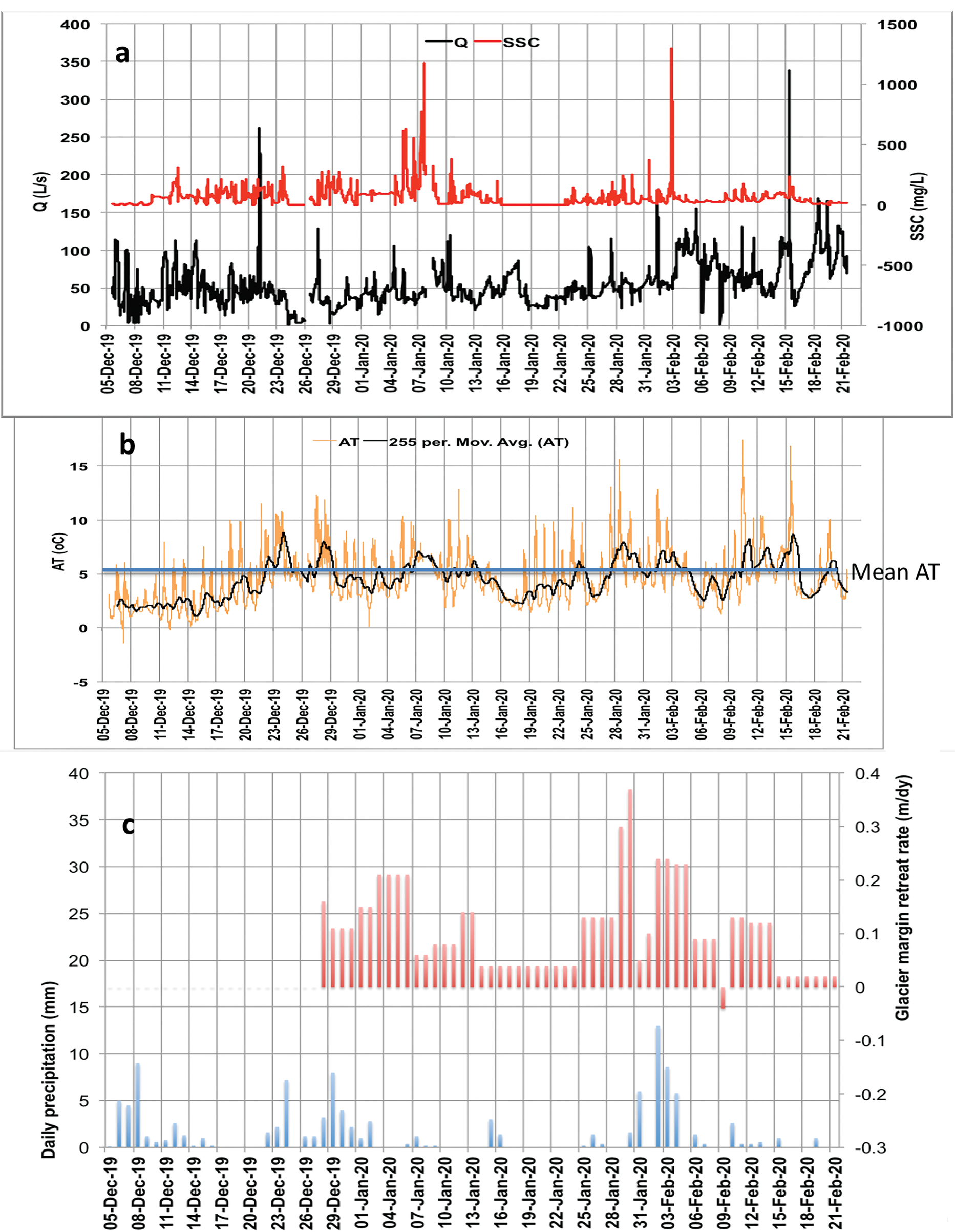
Fig. 6. a. The 5-min discharge (Q; black line) and suspended sediment concentration (SSC; red line) for 5 December 2019–21 February 2020. Note short gaps in the record on 26 December 2019 and 7–8 January 2020. b. The 5-min air temperature (AT) measured at the site (orange line) with the daily moving average (black line). Mean AT for the study period (blue line) was 4.5°C. c. Daily precipitation (blue bars) and glacier retreat distance (red bars).
Turbidity and suspended sediment concentration
For the entire study period, the gravimetrically determined SSCmean was 71.0 ± 15.9 mg l-1 (n = 454), with SSCmax 982.1 mg l-1 and SSCmin 0.1 mg l-1. For the 5 min SSC record estimated from turbidity, SSCmean was 58.8 ± 0.5 mg l-1 (n = 21 985) with SSCmax 1291.8 mg l-1 and SSCmin 0.1 mg l-1. That the SSCmax for the predicted 5 min SSC record is slightly higher than the calculated SSCmax from the 454 water samples suggests that some of the highest SSC events were not sampled by the portable sampling programme, or that extrapolation of the NTU record might have resulted in overestimation. However, inspecting Fig. 6a (red line), the two significant SSC peaks occurred on 7 January 2020 and from 2 to 3 February 2020, both lasting < 1 h.
There was snowfall of 0.15 m on Signy Island on 22–23 November, and this melted before the monitoring period started on 5 December. However, samples collected and analysed during this snow melt period gave a mean SSC value of 25.0 ± 5.3 mg l-1 (n = 19), which was significantly lower than that measured for the 5 December–21 February study period when SSCmean was 73.3 ± 16.5 mg l-1 (n = 438). It is probable that stream flow in the period 22 November–5 December was dominated by snow melt rather than ice melt and so had lower SSCs.
Suspended sediment dynamics
Figure 7 shows examples of Q and SSC time series plotted from the 5 min data for six events. Figure 7a & b show the SSC peaking before Q, indicating freely available sediment that was transport limited and denoting clockwise hysteresis. In Fig. 7c, d & f, SSC peaks after Q, indicating that sediment supply was limited, or from a distant source, and denoting anticlockwise hysteresis. In Fig. 7e, the SSC peak coincides with the Q peak (with small subsidiary peaks in SSC and Q on the falling limb of the hydrograph).

Fig. 7. Examples of discharge (Q) and suspended sediment concentration (SSC) time series for six events: a. 20–21 December 2019, b. 5 January 2020, c. 27 January 2020, d. 10–11 February 2020, e. 11 February 2020 and f. 15 February 2020.
Using the method described by Aich et al. (Reference Aich, Zimmermann and Elsenbeer2014), HI was calculated for 33 hydrographs during the study period, and these are plotted in Fig. 8a, with daily SSL plotted in Fig. 8b for comparison.

Fig. 8. a. Hysteresis index (HI) calculated using the method of Aich et al. (Reference Aich, Zimmermann and Elsenbeer2014) for 33 hydrographs during the study. b. Daily suspended sediment loads (SSLs; with error bars) for comparison with HI. Dates on a. and b. do not match and therefore the graphs do not align exactly.
Estimation of suspended sediment load
The sediment discharge by mass at a given time, Qs (mg s-1), is given by
 $${\rm Qs} = {\rm Qw } \times {\rm SSC}$$
where Qw is water discharge (l s-1) and SSC is in mg l-1. This 5 min value was scaled up per 5 min period, then the 288 daily 5 min periods were summed to give the daily SSL (kg) with SE = SD / √n. Figure 9 shows the calculated daily SSLs with SE bars, with daily Qmean (also with error bars) and daily ATmean plotted on the secondary axis. SSLs were very low for the first 4 days of the study period (5–9 December 2019), when temperature was low and snow/ice formed in the channel. Then came a rise in AT and a sharp increase in Q from 9 to 12 December 2019 with a corresponding increase in SSL to a peak SSL of 240.2 kg on 12 December 2019. The peak in SSL on 12 December is probably the first flush of sediment when Q was high enough to transport available sediment as the ice began to melt and subglacial sediment began to be released. After 12 December, there were snowfall events and low ATs, which partially froze the stream between 24 and 26 December and again between 16 and 21 January 2020. After the first SSL peak on 12 December, daily mean SSL remained < 150 kg, with just six other days when SSL exceeded that: 21 December (coinciding with rising Q and AT); 5–7 January 2020 were the 3 days with the highest SSLs of the season, with that of 7 January 2020 peaking at 378 kg; 2 February 2020; and 14 February 2020. All SSL peaks coincided with high AT and Q (Fig. 9).

Fig. 9. Daily suspended sediment loads (SSLs; with error bars) plotted alongside daily mean discharge (Q; with error bars) and air temperature (AT) for each day of the study.
To summarize, daily mean SSL was 75 ± 8 kg day-1 and ranged from 0 kg day-1 during two cold spells when the stream filled with snow and froze to 378 kg day-1 in mid-season.
Estimation of suspended sediment yield
The daily mean SSL was 75 ± 8 kg day-1 over the duration of the 79 day study. However, in order to be able to estimate the annual SSY, information about the length of the melt season is required. Monthly mean temperatures for Orcadas Station were examined for the period 2000–12 (13 years) and the average monthly mean AT was calculated for each month of the year. October–April had positive temperatures (1.6, 3.0, 4.4, 5.0, 5.0, 4.0, 1.7°C), while for the rest of the year from May to September monthly mean temperatures were negative (-0.3, -4.0, -5.8, -4.4, -1.4°C). If we therefore assume that on average snow and ice are melting on at least 6 (maximum of 7) months of the year on Signy Island (mid-October to mid-May), then we can assume that the estimated SSL is being transported for 6 months (182.5 days) of the year at the study site. The product of the daily SSL (75 ± 8 kg day-1) and the length of the melt season gives 13.7 t yr-1. The SE of the daily SSL is 8 kg day-1 or 10.7%, so applying this error to the annual total gives 13.7 ± 1.5 t yr-1.
In order to estimate the SSY, we need to divide this figure by the catchment area, which was estimated to be 0.32 km2. Combining these uncertainties with the SSY errors means that SSY could range between 34.9 and 52.2 t km-2 yr-1, with the mid-point between these upper and lower estimates being 43.6 t km-2 yr-1.
Glacier snow cover and precipitation
Snow melted sufficiently by 28 December to be able to accurately discern the glacier margin. From this point onwards in the study, measurements of the position of the ice margin were made every 2–3 days. Retreat rates increased to a maximum of 0.35 m day-1 by late January (Fig. 6c), after which point they began to decrease. A total of 112.3 mm of precipitation was recorded over the 79 day study period, with the daily mean being 1.4 mm day-1 and a maximum daily total of 13 mm, which was recorded on 2 February 2020 (Fig. 6c).
Model results
The Model 1 multiple regression statistics are summarized in Fig. 10a, and the Model 1 predictive equation used to generate the predicted SSL was as follows:
 $$\eqalign{& {\rm SSL\ } = -6.826 + 3.418 \times {\rm Q\ Hr\ } \gt 50 + 9.864 \cr & \quad \quad \quad\times {\rm A}{\rm T}_{{\rm mean}} \, \lpar {{\rm multiple}\,r = 0.54\comma \;\,r^2 = 0.30\comma \;\,n = 79} \rpar } $$
Figure 10b shows the model predicted SSL (red line) compared to the measured SSL (blue line) for the Orwell Glacier dataset (5 December 2019–21 February 2020). While the model generally worked for predicting medium and low SSLs, and the total predicted SSL for the measurement period matched that measured, it failed to account for the five SSL peaks in the study period, resulting in large underestimations for those 7 days. Hydroclimatic indices alone, therefore, as used in Model 1, could not account for sediment transport on those days. It was therefore decided to incorporate a sediment-based index, with SSCmean being the obvious choice (due to its high correlation coefficient with SSL; r 2 = 0.962, n = 79, P < 0.001), to build a second model (i.e. Model 2).

Fig. 10. a. Regression statistics for Model 1. b. Model 1 predicted suspended sediment loads (SSLs) compared with measured SSL. c. Regression statistics for Model 2. d. Model 2 predicted SSL compared with measured SSL. e. Model 2 + 1°C temperature increase scenario. f. Model 2 + 2°C temperature increase scenario. The graphs in d. shows the model predicted SSL (red line) compared to the measured SSL (blue line) for the Orwell Glacier dataset (5 December 2019–21 February 2020). This provided a much better fit than Model 1, but use of this model requires the additional input of mean suspended sediment concentration, which would involve further fieldwork to gather such data.
The Model 2 multiple regression statistics are summarized in Fig. 10c, and the Model 2 predictive equation used to generate the predicted SSL was as follows:
 $$\eqalign{& {\rm SSL\ } = -8.874 + 1.073 \times {\rm SS}{\rm C}_{{\rm mean}}- 0.79 \times {\rm A}{\rm T}_{{\rm mean}} \cr & \quad \quad\quad + 2.141 \times {\rm Q\ Hr\ } \gt 50 \,\, \lpar {{\rm multiple}\,\,r = 0.95\comma \;\, }\cr& \quad \quad \quad \,\,{ r^2 = 0.91\comma \;\,n = 79} \rpar } $$
Figure 10d shows the model predicted SSL (red line) compared to the measured SSL (blue line) for the Orwell Glacier dataset (5 December 2019–21 February 2020). This provided a much better fit than that for Model 1, but use of this model requires the additional input of SSCmean, which would involve further fieldwork to gather such data.
Global climate models such as the Hamburg climate model typically adopt changes in temperature and precipitation in the range from 1°C to 3°C and from –10 to +10%, respectively. By adding a linear trend line to the mean annual temperatures reconstructed for Signy Island (from Orcadas Station data; Fig. 11) we established that the mean annual temperature on Signy has risen from -1.5°C in 1910 to 1.2°C in 2020 (a rise of 0.25°C per decade). Extrapolating this would suggest that, by 2050, the mean annual temperature could be 0.75°C higher than in 2020 and +1°C by 2060 (compared with 2020). Mean annual temperatures on Signy Island would therefore be +2°C higher by 2100 than in 2020.

Fig. 11. Mean annual air temperature (AT) on Signy Island reconstructed from Orcadas Station data using relationship in Fig. 2c, with linear trend line. Data from http://www.nerc-bas.ac.uk/icd/gjma/orcadas.temps.html (accessed 2 March 2020).
In order to assess the effect of such future predicted rises in AT in the Antarctic on SSLs on Signy Island, Model 2 was run again with AT + 1°C (which, extrapolating the trend of a 0.25°C rise per decade over the past 110 years, would increase Q Hr > 50 by 23% by c. 2050) to give the output in Fig. 10e (a 6.5% increase in total SSL). For a +2°C temperature increase scenario (which would happen by 2100), Model 2 was run again with AT + 2°C (which would increase Q Hr > 50 by 47%) to give the output in Fig. 10f (a total of a 13% increase in SSL). However, it should be noted that these projected increases assume no change in SSCmean, but only a change in Q Hr > 50. It is improbable in temperature increase scenarios of +1°C and +2°C that the bed of the glacier would not change.
Discussion
Suspended sediment dynamics and hysteresis patterns
Figure 6 shows four distinct peaks in SSL and Q that need consideration. The first of these was a huge increase in Q on 21 December 2019, which did not coincide with any precipitation and did not significantly increase SSC. However, there was still a significant amount of snow on the glacier and there was a rise in AT on the previous day (20 December), which most probably caused rapid snow melt but transported very little suspended sediment. The SSC peak on 7 January 2020 is preceded by several other lower SSC peaks and coincides with above-average AT on 5 and 6 January, although not significantly high Q. This may be because by this time much of the snow on the glacier had melted (see Fig. 6c, red bars, which show that the ice at the glacier margin was snow free), so there was not a significant rise in Q, but perhaps subglacial channels had started to become active, hence the high SSC. The third significant SSC peak occurred on 3 February 2020 and coincided with the most significant precipitation event of the study period (see Fig. 6c, blue bars) and above-average AT in the preceding days. These conditions must have triggered this flush of suspended sediment. The fourth, and final, peak in Q occurred on 15 February 2020 and coincided with some of the highest ATs of the study. However, there was not a corresponding SSC peak, suggesting that suspended sediment may have been exhausted by this later stage in the melt season.
Figure 8a showed the calculated HI for 33 events compared with the daily SSL (with error bars) in Fig. 8b. The preponderance of negative (anticlockwise) HI values in Fig. 8a (21/33 or 64%) indicates that sediment transport in this stream was supply limited, or that the source of the sediment was far from the monitoring point (Klein Reference Klein1984), for most of the season. The two highest HI values were HI = 1.01 on 5 January 2020, which coincided with the highest SSLs of the season on 5–7 January, and HI = 0.73 on 21 December 2019, which coincided with a peak in SSL on that date (Fig. 8b). Aich et al. (Reference Aich, Zimmermann and Elsenbeer2014) used complete annual records to assess the trend of hysteresis loops during the meteorological year in their study in the Lutzito catchment on Barro Colorado Island, Panama, and they found in 2008 that HI values dropped from ~1.0 at the beginning of the rainy season to 0.5 at its end. In their study in the Estero Morales basin, a Chilean Andean basin with 7% glacier cover, Mao & Carillo (Reference Mao and Carrillo2017) reported that approximately half of the SSY was transported during the snow melt period and half during glacier melting. During snow melt, an unlimited supply of fine sediments was provided in the lower and middle parts of the basin and hysteresis patterns tended to be clockwise, as the peaks in SSC preceded the peak Q in daily hydrographs. During glacier melting, however, the source of fine sediments was the proglacial area, producing anticlockwise hysteresis. In this study at Orwell Glacier, however, the stream drains directly from under the ice, with no proglacial area for the stream to cross. The hysteresis patterns, and therefore sediment load, must therefore be governed by basal erosion and subglacial hydrological processes, which control the supply of sediment for transport. Indeed, Swift et al. (Reference Swift, Nienow and Hoey2005) found that sub-seasonal changes in relationships between suspended sediment transport and discharge demonstrated that the structure and hydraulics of the subglacial drainage system critically influenced how basal sediment was accessed and entrained. However, it should be noted that this glacier has extended and retreated over time, and retreat elsewhere on Signy Island (and more generally on the Antarctic Peninsula) at present is exposing old moss banks (Smith Reference Smith1982, Yu et al. Reference Yu, Beilman and Loisel2016), so it is highly probable that basal materials beneath the lower parts of glaciers such as Orwell Glacier would have been proglacial sediments before the glacier last advanced, sediments that are today being reworked by fluvial processes in summer as the ice margin retreats.
Future predictions of suspended sediment load in the Orwell Glacier meltwater stream based on multiple regression modelling
In order to assess the effect of future predicted rises in AT in the Antarctic on SSLs on Signy Island, Model 2 was run with AT + 1°C (which, extrapolating the trend of a 0.25°C rise per decade over the past 110 years, would increase Q Hr > 50 by 23% by c. 2050) to give the output in Fig. 10e (a 6.5% increase in total SSL). For a +2°C temperature increase scenario (which would happen by 2100), Model 2 was run again with AT + 2°C (which would increase Q Hr > 50 by 47%) to give the output in Fig. 10f (a total of a 13% increase in SSL). However, it should be noted that these projected increases assume no change in SSCmean, but only change in Q Hr > 50. It is improbable in temperature increase scenarios of +1°C and +2°C that the bed of the glacier would not change. In all likelihood there would be increased basal hydraulic connectivity (e.g. Perolo et al. Reference Perolo, Bakker, Gabbud, Moradi, Rennie and Lane2019), increased abrasion, scour and bedrock erosion and more ice melt higher up the glacier, all probably increasing the available sources of sediment that, with higher Q to transport it, would raise SSLs considerably more than those predicted by Model 2 (Fig. 10e & f). Indeed, Delaney & Adhikari (Reference Delaney and Adhikari2020) simulated synthetic alpine glaciers experiencing accelerated glacier melt for 100 years, and they found that sediment discharge increased by around eight times the steady glacier values by the end of the simulation.
Moragoda & Cohen (Reference Moragoda and Cohen2020) found that, at the end of this century, projected climate changes under Representative Concentration Pathways 2.6, 4.5, 6.0 and 8.5 scenarios will lead to 2.0%, 6.0%, 7.5% and 11.0% increases, respectively, in mean global river discharge relative to the 1950–2005 period, while mean global suspended sediment flux will show 11.0%, 15.0%, 14.0% and 16.4% increases, respectively, under pristine conditions. Our model predictions for Q in this study are higher (understandably, as the catchment is > 90% ice/snow covered), but our predicted increases in SSL (suspended sediment flux) are within those suggested by Moragoda & Cohen (Reference Moragoda and Cohen2020). Syvitski (Reference Syvitski2002) applied a model for predicting the sediment flux in ungauged river basins to 46 Arctic and sub-Arctic rivers. He found that for every 2°C of warming, the model predicted a 22% increase in the flux of sediment carried by rivers. For every 20% increase in water discharge, there would be a 10% increase in sediment load. These predictions agree quite well with those we have estimated for Signy Island.
Comparison of suspended sediment loads from Orwell Glacier with other studies
A selection of studies of sediment transport and SSYs from proglacial environments around the world is presented in Table IV. It should be noted that Table IV is not comprehensive, but the studies included are illustrative of the size of the SSYs that have been observed in these environments. The two Antarctic studies have SSYs that are considerably lower than those of any of the other regions, with the mean of this and the Ross Island study (Kavan et al. Reference Kavan, Ondruch, Nývlt, Hrbáček, Carrivick and Láska2017) being 115 t km-2 yr-1. The ten studies chosen from the Arctic region (Svalbard, Norway and Greenland) have a mean SSY of 1596 t km-2 yr-1, an order of magnitude higher than the Antarctic studies thus far undertaken. Although this difference may simply reflect the far greater number of studies that have been carried out in the Arctic, it highlights the need for more Antarctic studies. The seven Alpine and Rockies studies (from the French, Swiss and Austrian Alps and Canadian Rockies) have a considerably higher mean SSY of 5455 t km-2 yr-1, which may be explained by higher relief, steeper slopes/glaciers, different geology (tectonic uplift) and longer melt seasons. The two studies included in Table IV from the Himalayas show the highest SSYs, with the mean being 7643 t km-2 yr-1. An important factor influencing SSY is latitude. Studies in locations closer to the equator such as the Himalayas generally have higher temperatures, glaciers are at higher altitudes and discharge is greater. The melt season is longer and so combining higher Q with high SSC over a longer melt season inevitably produces the highest SSYs globally. In polar regions (Arctic and Antarctic), mean temperatures, and therefore Q, are much lower, as are the lengths of the melt seasons; therefore, SSYs are much lower. However, care should be taken when interpreting these data because, as Stott et al. (Reference Stott, Nuttall, Eden, Smith and Maxwell2008) pointed out, suspended sediment transport and SSYs change rapidly with distance from the glacier snout, so it is important to consider this when comparing studies. Table IV includes the proportion of each basin that is ice covered, which is an important consideration. In their study of 90 glacierized basins, Gurnell et al. (Reference Gurnell, Hannah, Lawler, Walling and Webb1996) concluded that basins containing predominantly warm-based glaciers produced higher SSYs than those containing predominantly cold-based glaciers (e.g. Orwell Glacier in this study). As SSYs in glaciated basins are elevated compared with those from non-glacial basins, they have been used as evidence for the increased efficacy of glacial erosion. However, it has been argued that a reliable relationship between glacial and non-glacial erosion rates on the basis of sediment yield has not yet been determined, with recognition that storage and release of sediment in proglacial channels may play a significant role in controlling these yield patterns (e.g. Warburton Reference Warburton1990, Orwin & Smart Reference Orwin and Smart2004, Geilhausen et al. Reference Geilhausen, Morche, Otto and Schrott2013, Leggat et al. Reference Leggat, Owens, Stott, Forrester, Déry and Menounos2015).
Table IV. Suspended sediment yields from studies in various proglacial environments.

a Suspended sediment yield in t km-2 yr-1 is calculated from SSL in t day-1 measured in the study (× 365 / basin area). It does not account for the variable length of melt seasons, so values are probably overestimates.
SSC = suspended sediment concentration, SSL = suspended sediment load; SSY = suspended sediment yield.
Conclusions
This study of suspended sediment transport at a glacier margin on a maritime Antarctic island is the first systematic study over a large part of the summer melt season. Daily mean SSL was 75 ± 8 kg day-1 and ranged from 0 kg day-1 during two cold spells when the stream filled with snow and froze to 378 kg day-1 in mid-season. From the 0.32 km2 basin that was 93% ice covered, we estimate that SSY could range between 34.9 and 52.2 t km-2 yr-1 over the 79 day study.
A multiple regression model using three predictive variables (daily mean SSC, daily mean AT and a stream discharge-based index) predicted the measured daily SSLs reliably (multiple r = 0.95, r 2 = 0.91, n = 79) and, when run with mean AT + 1°C and mean AT + 2°C scenarios, it predicted 7% and 13% increases in SSL, respectively, by 2100. As with all models of this nature, however, they make assumptions. These model predictions did not account for factors such as potential changes in the supply of sediment, changes in the amount, type and distribution of precipitation or changes in the physical extent (area, volume) of the glacier, all of which would affect the SSLs predicted in a warmer climate.
When compared with a further 18 studies from the Arctic, Alpine regions, the Andes, Rockies and Himalayas, the SSLs estimated in this study and another recent one from James Ross Island off the north-east Antarctic Peninsula are low by comparison. However, if recent climatic trends continue, as they are predicted to, then the findings from this study suggest that increases in SSL from maritime Antarctic glaciers can be expected in future.
Acknowledgements
Matt Jobson, station leader of Signy Research Station, is thanked for logistical support, and John Davies (British Antarctic Survey) helped with technical support in the field. Martin McCallum assisted with transporting field equipment. Laura Gerrish, British Antarctic Survey Mapping and Geographic Information Centre, assisted with the preparation of Fig. 1. Izzy Collins and Debbie Stott assisted with laboratory work and Liverpool John Moores University loaned equipment and approved sabbatical leave for TS. Thanks to Dr Jan Kavan and another anonymous reviewer for their helpful comments, which improved the final manuscript.
Author contributions
TS planned and conducted the fieldwork on Signy Island and wrote the first draft of the manuscript. PC collaborated in the original submission of the Collaborative Antarctic Science Scheme bid and in finalizing the manuscript prior to submission.
Financial support
TS was in receipt of a Natural Environment Research Council award through the Collaborative Antarctic Science Scheme (CASS project number 164) with the British Antarctic Survey (BAS). PC is supported by NERC core funding to the BAS ‘Biodiversity, Evolution and Adaptation’ Team.
Details of data deposit
All data are retained by the lead author.


