


Introduction
The Antarctic Peninsula (AP) is experiencing some of the most rapid climate changes on Earth (Turner & Marshall Reference Turner and Marshall2011). Over the last 50 years, a marked warming trend of mean surface air temperature (Turner et al. Reference Turner, Colwell, Marshall, Lachlan-Cope, Carleton, Jones, Lagun, Reid and Iagovkina2005) and increasing winter precipitation (Vaughan et al. Reference Vaughan, Marshall, Connolley, Parkinson, Mulvaney, Hodgson, King, Pudsey and Turner2003) have been observed. In the West Antarctic Peninsula, annual mean air temperatures have risen by ∼3°C since 1951 (Turner et al. Reference Turner, Colwell, Marshall, Lachlan-Cope, Carleton, Jones, Lagun, Reid and Iagovkina2005). The changing climate conditions are altering the glacial systems and duration of seasonal snow cover on ice-free areas, including significant retreat of glacier front positions (Rau et al. Reference Rau, Mauz, De Angelis, Jaña, Neto, Skvarca, Vogt, Saurer and Gossmann2004), break-up and disintegration of ice shelves (Cook & Vaughan Reference Cook and Vaughan2010) and subsequent speed-up of inland ice masses (Pritchard & Vaughan Reference Pritchard and Vaughan2007), increased meltwater production from glaciers (Vaughan Reference Vaughan2006), and a reduction of seasonal snow cover extent (Fox & Cooper Reference Fox and Cooper1998). However, observations of glacial systems show large spatial variability of these processes, e.g. Navarro et al. (Reference Navarro, Jonsell, Corcuera and Martín-Espanol2013) showed that mass loss from glaciers on Livingston Island has decelerated in the last decade (2002–11).
The dynamics of glaciers and snow cover are important components in polar ecosystems. Coastal ecosystems are strongly influenced by the amount of freshwater as well as induced suspended organic and inorganic matter transport into adjacent fjords and bays (Dierssen et al. Reference Dierssen, Smith and Vernet2002). Consequently, detailed information on glacier and snow extent and its variability over space and time, as well as quantification of meltwater and ice discharge, provide physical boundary conditions for ecological studies in polar environments. In order to model glacier mass balances and estimate ice mass flux and calving rates, information on glacier surface conditions, i.e. ablation patterns and firn line positions, and glacier surface velocities are required.
Recent spaceborne synthetic aperture radar (SAR) systems provide very high-resolution imagery, independent of solar illumination and cloud cover (Suess et al. Reference Suess, Riegger, Pitz and Werminghaus2002). They enable regular mapping of larger areas at short revisit times. In this paper, we demonstrate the potential of high-resolution X-band time series of the German TerraSAR-X (TSX) mission to: i) delineate the glacier extent for land-terminating glaciers by SAR coherence mapping (TSX HighResolution Spotlight (HS) imaging mode), ii) derive patterns of snow cover and their temporal dynamics on ice-free areas by SAR coherence mapping (TSX Stripmap (SM) imaging mode), iii) map glacier surface conditions from multi-temporal SAR intensity images (TSX SM imaging mode), and iv) determine ice velocities by SAR intensity feature-tracking and their integration into ice mass flux estimates (TSX HS and SM imaging mode).
Study site
King George Island (KGI) is the largest of the South Shetland Islands located north of the AP. More than 90% of the island area (1250 km2) is covered by glaciers (Simões et al. Reference Simões, Bremer, Aquino and Ferron1999), while the ice-free areas are concentrated in several larger peninsulas with rocky surfaces and sparse vegetation (Fig. 1). The ice-free Fildes, Barton and Potter peninsulas addressed in this study are relatively low in elevation. Their hydrological regime is dominated by glacial meltwater and snow meltwater from the ice-free areas themselves (Vogt & Braun Reference Vogt and Braun2004). The ice fields are drained by several tidewater glaciers, e.g. the Fourcade Glacier, calving into Potter Cove. The island is subject to a maritime polar climate with summer temperatures frequently above 0°C. Positive temperatures are also regularly observed during spring and autumn months (Rückamp et al. Reference Rückamp, Braun, Suckro and Blindow2011), and occasional warming events can even lead to snow melt during winter. Weather conditions change rapidly, related to a succession of eastward-moving low-pressure systems which transport relatively warm and humid air masses associated with frequent rain or snowfall and strong winds near the island’s coast (Bintanja Reference Bintanja1995).

Fig. 1 Overview map of King George Island (South Shetland Islands), Antarctica. a. Location of King George Island, Antarctic. b. Coverage of the various tracks and modes of TerraSAR-X data, arrows indicate the viewing direction, the red box marks the subset of the magnification of the study area shown in c. Background image: SPOT-4, 18 November 2010, © ESA TPM, 2010.
Data
Satellite data
A continuous time series of TSX SM data was acquired between October 2010 and April 2011 including the entire melt period of the spring and summer (Suess et al. Reference Suess, Riegger, Pitz and Werminghaus2002). The data covered the western part of KGI with the main ice cap, as well as several ice-free peninsulas (Fig. 1b). These data form the basis of our investigation of snow extent and glacier facies. In addition, two sets of TSX HS mode imagery (DLR 2009) were acquired over Potter Peninsula at the end of the summer season along ascending and descending paths to determine glacier extent and ice dynamics. As reference for the snow extent studies and location of the calving front of Potter Glacier, two acquisition scenes of the optical Satellite Pour l’Observation de la Terre (SPOT 4) were acquired on 18 November 2010 and 15 January 2011, covering the western part of KGI. For both dates, the imagery was available as multi-spectral and panchromatic datasets. An overview of all satellite data used in this study and their specific characteristics are given in Table I.
Table I Satellite data overview.

Differential GPS measurements
As field reference for the ice extent investigation from repeat TSX HS imagery, a differential GPS (DGPS) track was acquired along the edge of Polar Club Glacier, terminating on Potter Peninsula, on 28 February 2011. For the height calculations of the calving front, 50 DGPS static point measurements were carried out at two locations on Potter Peninsula opposite to Fourcade Glacier on 5 March 2011. The measurements were performed using NovAtel DL-4plus GPS receivers and NovAtel GPS-702-GG antennas. The permanent GPS point from the Argentine Carlini base (formerly named Jubany) was used as the base station. The baseline between the base and rover stations did not exceed 10 km, resulting in a horizontal accuracy of 0.02 m in static mode and a circular error probable of 0.20 m (NovAtel 2005).
Methodology
Synthetic aperture radar data pre-processing
All TSX data was ordered in single look complex (SLC) format with science orbits. Figure 2 shows the main processing steps for the various products. The respective details on azimuth and range resolutions are listed in Table I. Co-registration of SM and HS data was done by intensity cross-correlation using 512×512 image windows and a signal-to-noise (SNR) threshold of <7 to discard unreliable points. This led to standard deviation errors of <0.2 pixels for the co-registration of all image pairs. Intensity products were subsequently calibrated. After complex interferogram generation from the co-registered SLC images, the magnitude of coherence
 $$\left| \gamma \right|$$
of the two complex SAR values u
1 and u
2 was estimated with a 5×5 pixel moving window following the formula of Bamler & Hartl (Reference Bamler and Hartl1998):
$$\left| \gamma \right|$$
of the two complex SAR values u
1 and u
2 was estimated with a 5×5 pixel moving window following the formula of Bamler & Hartl (Reference Bamler and Hartl1998):
 $$\!\mid\!\gamma \!\mid\,={{\,\mid\!\mathop{\sum}\nolimits_{n\,=\,1}^L {u_{1} } (n)u_{2}^{{\asterisk}} (n)\!\mid\,} \over {\sqrt {\mathop{\sum}\nolimits_{n\,=\,1}^L {\!\mid\!u_{1} (n)\!\mid^{2} \mid\!u_{2} (n)\!\mid^{2} } } }},$$
where a sum Σ of independent samples L is used to estimate the maximum likelihood of
 $$\left| \gamma \right|$$
. The SM imagery was multi-looked to a ground range pixel size of 5 m and HS imagery to a ground range pixel size of 3 m to reduce speckle effects. All processed intensity/coherence images and displacement fields were geocoded on an improved digital elevation model (DEM) in 50 m resolution provided by Braun et al. (Reference Braun, Simões, Vogt, Bremer, Blindow, Pfender, Saurer, Aquino and Ferron2001) and Blindow et al. (Reference Blindow, Suckro, Rückamp, Braun, Schindler, Breuer, Saurer, Simoes and Lange2010). The poor resolution and accuracy of the DEM in the area of Potter Cove limited exact positioning and overlay of the different orbit paths.
$$\left| \gamma \right|$$
. The SM imagery was multi-looked to a ground range pixel size of 5 m and HS imagery to a ground range pixel size of 3 m to reduce speckle effects. All processed intensity/coherence images and displacement fields were geocoded on an improved digital elevation model (DEM) in 50 m resolution provided by Braun et al. (Reference Braun, Simões, Vogt, Bremer, Blindow, Pfender, Saurer, Aquino and Ferron2001) and Blindow et al. (Reference Blindow, Suckro, Rückamp, Braun, Schindler, Breuer, Saurer, Simoes and Lange2010). The poor resolution and accuracy of the DEM in the area of Potter Cove limited exact positioning and overlay of the different orbit paths.

Fig. 2 Flow chart of the TerraSAR-X (pre-)processing steps required to generate the various products. MLI=multilayer insulation.
Glacier extent by multi-temporal coherence images
Coherence images of TSX HS image pairs with 11 and 22 days repetition time were utilized to investigate the extent of Polar Club Glacier. Coherence is lost rapidly on glacier surfaces because of melting processes, snowfall, redistribution of snow by wind and glacier flow (e.g. Strozzi et al. Reference Strozzi, Luckman, Murray, Wegmuller, Werner and Werner2002, Atwood et al. Reference Atwood, Meyer and Arendt2010). These processes generally limit the application of SAR interferometry, but coherence analysis can be used in an inverse approach since rocks, bare soil and sparsely vegetated surfaces bordering the glacier frequently remain coherent over shorter time intervals of days up to a few weeks (Weydahl Reference Weydahl2001). Consequently, low coherence can be used to delineate glacier extent. As snow cover is also characterized by low coherence related to volumetric and temporal decorrelation (Atwood et al. Reference Atwood, Meyer and Arendt2010), TSX HS images of the late summer period (end of February until beginning of March) were used to determine the glacier extent, when most of the snow cover on the glacier-free areas had melted.
A binary glacier mask was generated from TSX coherence images by applying a threshold of
 $$\left| \gamma \right|$$
<0.3. This mask still includes incoherent meltwater lakes forming on the ice-free areas as well as remaining incoherent snow cover spots. In a subsequent processing step, only areas connected to glaciers were used, and glacial lakes fed by the glacial meltwater were masked using a threshold in the SAR intensity image. The method works only between glacier surface and land areas since oceans also decorrelate over time and inhibit a separation via SAR coherence.
$$\left| \gamma \right|$$
<0.3. This mask still includes incoherent meltwater lakes forming on the ice-free areas as well as remaining incoherent snow cover spots. In a subsequent processing step, only areas connected to glaciers were used, and glacial lakes fed by the glacial meltwater were masked using a threshold in the SAR intensity image. The method works only between glacier surface and land areas since oceans also decorrelate over time and inhibit a separation via SAR coherence.
The glacier front of Polar Club Glacier, terminating on Potter Peninsula, measured by DGPS was used as ground truth of the generated glacier masks. Glacier border lines generated from TSX HS image pairs in ascending and descending orbit directions were compared to each other in order to assess the methodology and influence of the coarse DEM on geolocation accuracy.
Snow cover mapping on ice-free areas by multi-temporal coherence images
Snow extent on the ice-free areas of the Potter, Barton and Fildes peninsulas was estimated by multi-temporal SAR coherence mapping. Coherence images were produced in 11-day intervals from the TSX SM time series between 25 October 2010 and 19 April 2011. Binary maps of incoherent (mainly snow and water) and other surfaces (primarily rocks, bare soil and vegetated areas) were generated with the same coherence threshold (
 $$\left| \gamma \right|$$
<0.3) as already mentioned for the glacier extent maps.
$$\left| \gamma \right|$$
<0.3) as already mentioned for the glacier extent maps.
Snow mapping results were evaluated by defining snow-covered and snow-free areas on two multi-spectral SPOT scenes (18 November 2010, 15 January 2011) by supervised classification. Those reference areas were compared to areas with
 $$\left| \gamma \right|$$
<0.3 and
$$\left| \gamma \right|$$
<0.3 and
 $$\left| \gamma \right|$$
>0.3 of TSX image pairs 16 November 2010/27 November 2010 and 10 January 2011/21 January 2011.
$$\left| \gamma \right|$$
>0.3 of TSX image pairs 16 November 2010/27 November 2010 and 10 January 2011/21 January 2011.
Glacier facies from multi-temporal RGB composites
The SAR imagery can be applied to map glacier zones based on their specific backscatter characteristics, related to liquid water content, grain size, snow density, stratigraphy and surface roughness (Partington Reference Partington1998). We adapted the radar glacier zone concept introduced by Rau et al. (Reference Rau, Braun, Friedrich, Weber and Goßmann2000) and Braun et al. (Reference Braun, Rau, Saurer and Gossmann2000) for C-band SAR data to KGI. The application of backscatter coefficient thresholds to classify radar glacier zones has been successfully applied in several studies using C-band imagery on the AP (e.g. Arigony-Neto et al. Reference Arigony-Neto, Saurer, Simões, Rau, Jaña, Vogt and Gossmann2009). The following radar glacier zones are distinguished in this study by backscatter intensities and elevation information: i) bare ice radar zone, ii) wet snow radar zone and iii) frozen percolation radar zone. The extents of bare ice areas and melt areas are of particular interest since they can be used as spatial reference for glacier surface mass balance modelling.
Following the method described by Partington (Reference Partington1998), the late summer snow line position can be identified from an RGB (red/green/blue) false composite using a TSX SM late winter image in a red, a summer image in a green, and a winter image in a blue colour channel. The multi-temporal RGB composite can then be used to visually differentiate the radar glacier zones in different colours, as well as an input for standard image classification approaches. The firn line was extracted and superimposed on the DEM to determine the mean altitude of the firn line position.
Glacier surface flow velocities from intensity feature-tracking
To determine surface flow velocities of Fourcade Glacier, intensity feature-tracking was carried out using the intensity cross-correlation algorithms described by Strozzi et al. (Reference Strozzi, Luckman, Murray, Wegmuller, Werner and Werner2002). All TSX SM image pairs with 11-day repeat intervals, as well as all TSX HS image pairs with 11 and 22 days repetition time, were processed. The success of surface displacement mapping by feature-tracking depends on the presence of nearly identical structures in the two images at the size of the employed tracking window (Strozzi et al. Reference Strozzi, Luckman, Murray, Wegmuller, Werner and Werner2002). Best results were achieved with a tracking window size of 128×128 pixels and a step size of 25 pixels. In order to only keep significant correlation results, an SNR threshold of seven was applied. Tracking results with lower SNR values were discarded due to low reliability. The generated velocity fields contain a global error from image co-registration, and a local error from feature-tracking. Quality assessment of the velocity fields was done on stable areas (e.g. rocks), where motion is expected to be zero.
Mass flux estimation
The calving rate at the calving front
 $$\dot{\hskip-2pt M}_{f} $$
is calculated from the averaged glacier velocity u
f
close to the front, and the width W, and the height H of the calving front according to Bamber & Payne (Reference Bamber and Payne2004):
$$\dot{\hskip-2pt M}_{f} $$
is calculated from the averaged glacier velocity u
f
close to the front, and the width W, and the height H of the calving front according to Bamber & Payne (Reference Bamber and Payne2004):
 $$\dot{\hskip-2ptM}_{f} {\,=\,}u_{f} W.$$
Surface velocities u
s
derived from feature-tracking on TSX images were applied to calculate ice mass flux at the calving front. Basal sliding and bed deformation are assumed to play a major role in the flow behaviour of Fourcade Glacier as its bed consists of volcanic rocks and sediments (Tokarski Reference Tokarski1987), and the ice cap is considered to be temperate in most parts (Macheret & Moskalevsky Reference Macheret and Moskalevsky1999). With this assumption, velocities averaged over depth
 $$\bar{u}$$
are set to be equal to observed surface velocities u
s
(Paterson Reference Paterson1994). A buffer of 40 m from the calving front towards the inner glacier part was applied to calculate mean surface velocities. The ice front width W was manually digitized from the TSX HS scene from 7 March 2011 and the panchromatic SPOT scene from 15 January 2011. The ice front height H was estimated by an intercept theorem applying basic geometrical calculations (schematic see Fig. 3) using the DGPS field measurements. One DGPS device
$$\bar{u}$$
are set to be equal to observed surface velocities u
s
(Paterson Reference Paterson1994). A buffer of 40 m from the calving front towards the inner glacier part was applied to calculate mean surface velocities. The ice front width W was manually digitized from the TSX HS scene from 7 March 2011 and the panchromatic SPOT scene from 15 January 2011. The ice front height H was estimated by an intercept theorem applying basic geometrical calculations (schematic see Fig. 3) using the DGPS field measurements. One DGPS device
 $$F{\tf="TNR"\char"A9}_{j} $$
was fixed on a tripod to determine the reference height RH. The other DGPS device was mounted on a mobile pole P
k
together with a Nikon Laser 550A5 range finder. The respective upper
$$F{\tf="TNR"\char"A9}_{j} $$
was fixed on a tripod to determine the reference height RH. The other DGPS device was mounted on a mobile pole P
k
together with a Nikon Laser 550A5 range finder. The respective upper
 $$G{\tf="TNR"\char"A9}_{j} $$
and lower point G
j
of the ice front were aimed through the range finder and brought in line with RH. The distances between DGPS measuring points and the calving front (
$$G{\tf="TNR"\char"A9}_{j} $$
and lower point G
j
of the ice front were aimed through the range finder and brought in line with RH. The distances between DGPS measuring points and the calving front (
 $$\overline{{{P_{k} G_{j} } }} $$
) were derived from the TSX HS scene from 7 March 2011 and the SPOT scene from 15 January 2011. Combining all data, the height of the calving front was calculated using the formula for intercept theorem:
$$\overline{{{P_{k} G_{j} } }} $$
) were derived from the TSX HS scene from 7 March 2011 and the SPOT scene from 15 January 2011. Combining all data, the height of the calving front was calculated using the formula for intercept theorem:
 $${{\overline{{P_{k} G_{j} }} } \over {\overline{{P_{k} F_{i} }} }}={{\overline{{G_{j} G{\tf="TNR"\char"A9}_{j} }} } \over {\overline{{F_{i} F{\tf="TNR"\char"A9}_{i} }} }}.$$
This procedure was applied for 50 DGPS points along the calving front of Fourcade Glacier. Additionally, an oblique digital photograph of the ice front was used to support the interpolation of the ice front heights. (The observation lines from two reference points are indicated in Fig. 9.)
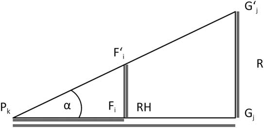
Fig. 3 Principle of the calculation of the calving front height by intercept theorem. H denotes the calving front height, Gj and G'j the lower and upper point of the calving front, RH the reference height, F'i the fixed differential GPS measuring point, and Pk the observer position at the mobile differential GPS measuring point.
The error magnitude of mass flux computation
 $$\Delta\, \dot{\hskip-2ptM}_{f} $$
is a function of
$$\Delta\, \dot{\hskip-2ptM}_{f} $$
is a function of
 $$\Delta u\,_{f} $$
,
$$\Delta u\,_{f} $$
,
 $$\Delta W$$
and
$$\Delta W$$
and
 $$\Delta H$$
. The impact of each individual error term on
$$\Delta H$$
. The impact of each individual error term on
 $$\dot{\hskip-2ptM}_{f} $$
was calculated by the Gaussian error propagation after Schönwiese (Reference Schönwiese2000):
$$\dot{\hskip-2ptM}_{f} $$
was calculated by the Gaussian error propagation after Schönwiese (Reference Schönwiese2000):
 $$\Delta\, \dot{\hskip-2ptM}_{f} {\,=\,}\sqrt {\left( {{{\partial \,\dot{\hskip-2ptM}_{f} } \over {\partial u_{f} }}\Delta u_{f} } \right)^{\!\!2} \!{\plus}\left( {{{\partial \dot{M}_{f} } \over {\partial W}}\Delta W} \right)^{\!\!2} {\plus}\left( {{{\partial\, \dot{\hskip-2ptM}_{f} } \over {\partial H}}\Delta H} \right)^{\!\!2} ,} $$
with
 $${{\partial\, \dot{\hskip-2ptM}_{f} } \over {\partial u_{f} }}$$
,
$${{\partial\, \dot{\hskip-2ptM}_{f} } \over {\partial u_{f} }}$$
,
 $${{\partial \,\dot{\hskip-2ptM}_{f} } \over {\partial W}}$$
,
$${{\partial \,\dot{\hskip-2ptM}_{f} } \over {\partial W}}$$
,
 $${{\partial\, \dot{\hskip-2ptM}_{f} } \over {\partial H}}$$
as the partial derivatives of
$${{\partial\, \dot{\hskip-2ptM}_{f} } \over {\partial H}}$$
as the partial derivatives of
 $$\dot{\hskip-2ptM}_{f} =u_{f} WH$$
.
$$\dot{\hskip-2ptM}_{f} =u_{f} WH$$
.
Results
Glacier extent
The binary coherence mask generated from the TSX HS image pair 5 March 2011 and 16 March 2011 is shown in Fig. 4a. The front lines of the Polar Club Glacier generated from TSX HS coherence images in ascending (track 104: 5 March 2011, 16 March 2011, green line), and descending path direction (track 125: 7 March 2011, 18 March 2011, red line), and the reference line measured by DGPS on 28 February 2011 (blue) are shown in Fig. 4b. All glacier borders show a high degree of consistency and indicate that the glacier border can be well distinguished from late summer TSX HS coherence pairs. The mean offset between glacier borders generated by coherence mapping and the reference line from DGPS measurements is±25 m, while the largest difference is ~240 m. Offsets between glacier border lines generated on TSX HS image pairs with opposite orbit direction can be observed in the western and eastern parts close to the coastline, and also south-east of the glacial lake area. These offsets show a maximal discrepancy of 180 m.

Fig. 4a Binary coherence mask generated from TerraSAR-X HighResolution Spotlight (TSX HS) image pair 5 March 2011/16 March 2011. Ice-free Potter Peninsula (<0.3)= black, water and glacier surfaces (>0.3)=white. b. Front lines of Polar Club Glacier generated from TSX HS coherence image pair 5 March 2011/16 March 2011 in ascending orbit direction (green), 7 March 2011/18 March 2011 in descending orbit direction (red), differential GPS reference measurements 28 February 2011 (blue). Background image: TSX HS 16 March 2011, © DLR, 2011.
Snow cover extent on ice-free areas
We compared the snow cover development and method performance of three main glacier-free peninsulas on KGI: namely Potter (mean elevation 62 m a.s.l., size 8 km2), Barton (mean elevation 119 m a.s.l., size 9.5 km2) and Fildes (mean elevation 44 m a.s.l., size 17 km2). The proportion of snow-covered area (
 $$\left| \gamma \right|$$
<0.3) is decreasing over the summer on the ice-free peninsulas (Fig. 5a–c). On Potter Peninsula, the percentage of snow-covered area was already low (~40%) by the end of November 2010, while 64% of Fildes and Barton were still snow-covered (Fig. 5a). In mid-January 2011, snow-covered areas were also decreasing on Barton (31%) and Fildes (34%) (Fig. 5b). Maximum extent of snow-free areas on all three peninsulas was reached in the first half of March 2011 (Fig. 5c), and decreased significantly at the beginning of April 2011 (Fig. 5d).
$$\left| \gamma \right|$$
<0.3) is decreasing over the summer on the ice-free peninsulas (Fig. 5a–c). On Potter Peninsula, the percentage of snow-covered area was already low (~40%) by the end of November 2010, while 64% of Fildes and Barton were still snow-covered (Fig. 5a). In mid-January 2011, snow-covered areas were also decreasing on Barton (31%) and Fildes (34%) (Fig. 5b). Maximum extent of snow-free areas on all three peninsulas was reached in the first half of March 2011 (Fig. 5c), and decreased significantly at the beginning of April 2011 (Fig. 5d).

Fig. 5a–d Temporal and spatial course of coherence on the Fildes, Barton and Potter peninsulas. Background image: SPOT-4, 15 January 2011, © ESA TPM, 2010.
The temporal development of snow-covered area percentage on all three peninsulas from November 2010 until April 2011 related to climate data of the Carlini (Potter Peninsula) (Servicio Meteorológico Nacional 2011) and Bellingshausen (Fildes Peninsula) (Arctic and Antarctic Research Institute 2011) meteorological stations are shown in Fig. 6. On average, the area percentage with
 $$\left| \gamma \right|$$
<0.3 in relation to total area of the respective peninsula is lowest on Potter (33%), and higher on Barton (43%) and Fildes (45%). The accuracy of coherence snow cover mapping is moderate in November, but high errors occur in January (Fig. 7). Of the areas classified as snow-covered or snow-free in the 18 November 2010 SPOT scene, 63% and 71%, respectively, were also revealed by coherence algorithms for the period between 16 November 2010 and 27 November 2010 (Fig. 7a–c). For January 2011, only 34% of area classified as snow-covered in the 15 January 2011 SPOT scene was defined as snow-covered in the TSX coherence image 10 January 2011/21 January 2011. In comparison, 86% of the area classified as snow-free in the SPOT scene was identified correctly by the coherence algorithms (Fig. 7d–f).
$$\left| \gamma \right|$$
<0.3 in relation to total area of the respective peninsula is lowest on Potter (33%), and higher on Barton (43%) and Fildes (45%). The accuracy of coherence snow cover mapping is moderate in November, but high errors occur in January (Fig. 7). Of the areas classified as snow-covered or snow-free in the 18 November 2010 SPOT scene, 63% and 71%, respectively, were also revealed by coherence algorithms for the period between 16 November 2010 and 27 November 2010 (Fig. 7a–c). For January 2011, only 34% of area classified as snow-covered in the 15 January 2011 SPOT scene was defined as snow-covered in the TSX coherence image 10 January 2011/21 January 2011. In comparison, 86% of the area classified as snow-free in the SPOT scene was identified correctly by the coherence algorithms (Fig. 7d–f).

Fig. 6 Temporal course of areas with <0.3 (incoherent/snow-covered) on the Fildes, Barton and Potter peninsulas from November 2010 to April 2011. Related meteorological data from the Carlini/Jubany (Potter) and Bellingshausen (Fildes) meteorological stations is superimposed.

Fig. 7 Snow coverage in November 2010 and January 2011 on Potter Peninsula. a. Panchromatic SPOT scene 18 November 2010, © ESA TPM, 2010. b. Binary coherence mask of TerraSAR-X Stripmap (TSX SM) 16 November 2010 to 27 November 2010. c. Snow coverage results of SPOT 18 November 2010 and TSX SM 16 November 2010 to 27 November 2010. d. Panchromatic SPOT scene 15 January 2011, © ESA TPM, 2010. e. Binary coherence mask of TSX SM 10 January 2011 to 21 January 2011. f. Snow coverage results of SPOT 15 January 2011 and TSX SM 10 January 2011 to 21 January 2011.
Glacier facies
The late summer snow line position was identified from a RGB false composite using the TSX SM late winter image (25 October 2010) in a red, the summer image (30 December 2010) in a green, and the winter image (28 March 2011) in a blue colour channel. The classification of radar glacier zones by the use of backscatter coefficient thresholds from SAR images was beset with great uncertainties and did not agree with field observations. For this reason, radar glacier zones were derived from the multi-temporal colour composite generated from TSX SM intensity images (Fig. 8). Backscatter coefficients on bare glacier areas are similar in spring (25 November 2010) and autumn/winter (28 March 2011) acquisitions and slightly lower in summer (30 December 2010). The approximate mean firn line altitude was identified at the 220 m contour line.

Fig. 8 Multi-temporal RGB composite of the Warszawa Icefield with TerraSAR-X Stripmap (TSX SM) intensity image 25 October 2010 in the red, 30 December 2010 in the green, 28 March 2011 in the blue channel. The bare ice radar zone is shown in green, the wet snow radar zone is blue and the frozen percolation radar zone is purple. The firn line position (FLP) is located at approximately 220 m a.s.l.
Glacier flow velocities
Glacier movement could be mapped by feature-tracking on TSX HS image pairs in areas of sufficient surface structures. Major glacier movement can be observed where Fourcade Glacier flows south-west into Potter Cove. Surface velocities at the calving front reached up to 1.8 m d-1 and decreased with increasing distance from the calving front (Fig. 9). Very slow displacement could be observed at the western part of the calving front where the surface is less inclined, and a sub-glacial trough exists. Surface velocities derived from TSX HS tracks in ascending (104) and descending (125) orbit directions are similar in magnitude but differ in coverage. The area of major ice flow of the Fourcade Glacier could not be tracked well on HS image pairs of track 104 due to SAR layover effects, which arise when the sensor measures in sloped surface topography. It is a relief distortion in the projection of the radar imagery due to the shorter run-time of the measuring wave-front to mountain top than to its foot. A slight mountain slope facing towards the SAR sensor will seem shorter or the mountain top and foot will be superimposed (foreshortening effect). If the mountain slope is very steep, this effect can get more extreme and the top will overlay the foot projection.

Fig. 9 Displacement field derived from TerraSAR-X track 104, 125 and 119. Mean surface velocities for 22 February 2011 to 18 March 2011 overlaid on the HS intensity image (7 March 2011), track 125, 3 m resolution. In situ measurements of the glacier calving front to distinctive points, i.e. line-of-sight from the differential GPS base station, are displayed in light-blue. Background image © DLR, 2011.
Using the TSX SM time series, surface displacement along the glaciated coast line could be tracked, whereas only few surface offsets were measured in the inner part of the ice cap with few to no surface structures (Fig. 10). For Fourcade Glacier, a maximum velocity of 1.2 m d-1 was mapped on TSX SM pairs from 23 February 2011 to 6 March 2011 and 6 March 2011 to 17 March 2011. The displacements are in the same order of magnitude as those obtained from feature-tracking on TSX HS image pairs, but the area of major movement of Fourcade Glacier could not be mapped well due to geometry constraints. In contrast, surface displacement was mapped on TSX SM image pairs for some parts of the south-western slopes close to the calving front, where no surface displacement could be generated from the TSX HS data of track 125. Consequently, tracking results of all three tracks were combined in order to achieve the most complete displacement field of the Fourcade Glacier and calculate its calving rates. The global error component for displacement measurements is <±0.02 m d-1 for HS and <±0.03 m d-1 for SM image pairs according to co-registration accuracy. Local offset-tracking on the ice-free area of Potter Peninsula on HS image pairs resulted in a mean surface velocity of 0.006 m d-1 with a standard deviation of 0.005 m d-1. For TSX SM image pairs, mean surface velocity on the ice-free area was one order of magnitude higher: 0.025 m d-1 with a standard deviation of 0.026 m d-1. Accordingly, the total error margin of the derived surface velocities is estimated at±0.02 m d-1.

Fig. 10 Displacement field derived from TerraSAR-X Stripmap (TSX SM) track 119. Mean surface velocities of the image pairs 23 February 2011/6 March 2011 and 6 March 2011/17 March 2011. The map excerpt of King George Island is indicated by the red rectangle in Fig. 1. Background: SM intensity image (30 December 2010), track 119, 3 m resolution, © DLR, 2010.
For the time period from February to March 2011, the volume flux of Fourcade Glacier was estimated at 20 700±5500 m3 d-1 or 4±1 m3 d-1 per metre glacier front length. Multiplying the flux
 $$\dot{\hskip-2ptM}_{f} $$
with the density of ice p
i
(≈917 kg m-3, Paterson Reference Paterson1994) results in a mass flux rate
$$\dot{\hskip-2ptM}_{f} $$
with the density of ice p
i
(≈917 kg m-3, Paterson Reference Paterson1994) results in a mass flux rate
 $$\dot{M}_{c} $$
of ∼19±5 kt d-1.
$$\dot{M}_{c} $$
of ∼19±5 kt d-1.
Discussion
Glacier extent
In the western and eastern parts of KGI, glacier fronts obtained from SAR coherence are similar in shape, but shifted spatially. These offsets are attributed to different viewing geometry of the SAR and respective geometrical distortion related to low quality and poor resolution of the DEM used for geocoding. The offsets located south-west of the lake area in the front of the glacier on Potter Peninsula can be attributed to temporal decorrelation caused by melting processes, rain/snow events or material redistribution through heavy wind. Additionally, due to the high degree of water saturation and slush conditions at some areas at the glacier margin the DGPS reference track is also not 100% coincident with the glacier border and, hence, absolute errors of the coherence glacier mask might even be smaller. The overall accuracy of determining the glacier extent from multi-temporal coherence images is moderate but high errors occurred related to the reasons stated above.
Snow cover extent on ice-free areas
The depletion of snow cover over the summer period can be clearly recognized in the temporal changes of binary coherence masks on the peninsulas. Areas of low coherence decrease over the summer when temperatures often rise above 0°C (Fig. 6) and melting occurs. The meteorological conditions between the peninsulas show significant spatial differentiation related to their exposure to incoming air masses (Kejna et al. Reference Kejna, Láska and Caputa1998), resulting in different amounts of accumulation and snow melt. In times of advection from the north and north-west, the predominant state on KGI (Martianov & Rakusa-Suszczewski Reference Martianov and Rakusa-Suszczewski1989), air temperatures on Fildes are lower than on Barton and Potter peninsulas because of foehn-type effects occurring at the elevation of the Arctowski Icefield (Kejna et al. Reference Kejna, Láska and Caputa1998). Furthermore, those prevailing advection directions, bringing humid and relatively warm air masses towards the northern part of the ice cap, cause higher cloud coverage and precipitation on Fildes Peninsula (Braun Reference Braun2001). This spatial difference can be recognized in the pattern of the temporal and spatial variability of SAR coherence. On Potter Peninsula, the area percentage with
 $$\left| \gamma \right|$$
<0.3 on average was lowest and started to decrease earlier than on the neighbouring peninsulas.
$$\left| \gamma \right|$$
<0.3 on average was lowest and started to decrease earlier than on the neighbouring peninsulas.
These findings can be related to higher air temperatures observed at Carlini Station during the investigation time period (Fig. 6). At Bellingshausen Station air temperatures were, on average, 0.5°C lower and daily amplitudes were less pronounced. The average sum of precipitation was twice as high as at Carlini Station. Those climatic conditions explain why snow cover depleted later and to a lesser extent on Fildes Peninsula. However, changes in coherence loss within the 11-day interval can also be caused by other factors, such as precipitation, thawing, water saturated permafrost and related ground movements, or by formation of meltwater lakes.
Classification results for snow-covered and snow-free areas of SPOT images and respective TSX coherence images differ in their spatial extent and distribution (Fig. 7). Part of this divergence can be explained by geometrical distortions in the TSX imagery introduced by the low accuracy of the DEM leading to spatial offsets between the optical and coherence images, especially in steep terrain. As discussed above, temporal loss of coherence during the 11-day acquisition interval can also be caused by weather events, changing dielectrical and structural characteristics of the surface, and hence reflect true changes, while the SPOT data provides information from a distinct date. Increases of meltwater surfaces are also included in the coherence maps, but they are not covered with the optical data. In November 2010, unstable weather conditions with the occurrence of heavy rainfall and high wind speeds decreased coherence. For this reason, areas defined as snow-free in the SPOT scene but defined as snow-covered by the coherence algorithms are distributed more or less evenly over the whole Potter Peninsula (Fig. 7c). Weather conditions in January 2011 were relatively stable with almost no precipitation and low wind speeds. Consequently, coherence was maintained and those areas classified as snow-free in the SPOT scene but defined as snow-covered in the TSX coherence image are mostly located on water surfaces (Fig. 7f). Snow cover mapping from coherence images remains difficult as accuracy results are only moderate to poor. The analysis shows that climate data support the interpretation of coherence images as well as other information, e.g. the location of meltwater lakes.
Glacier facies
The analysis of the time series of TSX SM data revealed considerable ambiguities for classification of radar glacier zones according to the concept developed on C-band data (e.g. Rau et al. Reference Rau, Braun, Friedrich, Weber and Goßmann2000, Arigony-Neto et al. Reference Arigony-Neto, Saurer, Simões, Rau, Jaña, Vogt and Gossmann2009). According to Rayleigh’s law of scattering processes, the radiated power of the backscatter signal is reciprocal proportional to the 4th power of the wavelength. Due to its shorter wavelength, the X-band backscatter signal is more sensitive to changes of surface roughness during wet snow conditions than is C-band. For wet snow penetration, depth is almost negligible, and surface scattering can become a dominant process depending on surface roughness. This was observed at various occasions in the time series with periods of pronounced topographically induced wind effects causing local patterns of rough (bright) surfaces that prevent a continuous analysis of melt surfaces. Additional influences were caused by local topographical effects leading to variable backscatter signals depending on the local incident angle. The best potential for identification of the firn line was in early winter imagery, acquisition dated from 28 March 2011 or 8 April 2011 (Fig. 5), when temperatures showed a clear drop below the melting point and fresh, fine-grained and transparent snow started to cover firn and bare ice areas.
By contrast, radar glacier zones and the firn line of the Warszawa Icefield can be visually identified in the multi-temporal SAR colour composite. A significant jump from autumn to winter backscatter can be observed at the firn line because cold temperature prevailed at the end of March leading to high volume scattering from the frozen firn. Areas above the firn line show up in blue (wet snow conditions in November and December with low backscatter) and purple (wet snow in December, frozen snow with high backscatter in November). Our finding of the mean firn line altitude at ~220 m is consistent with findings from previous years defined by Braun & Rau (Reference Braun and Rau2000) using ERS-1/-2 SAR late summer images (1992–99) for the north-western part of the ice cap. They defined the firn line position of glacier areas near Fildes Peninsula between 180 and 270 m a.s.l.
Glacier flow velocities
The magnitude of surface velocities derived from TSX HS track 125 and 104 remains stable for image pairs with 11 or 22 day time intervals, indicating that the tracking results are reliable. This is further confirmed by the fact that surface velocities derived from TSX SM image pairs, covering the same time period and area, are in the same order of magnitude as TSX HS datasets. Differences in location and extent of tracking results between the different tracks can be explained by the satellite path direction and the associated viewing geometry. Very steep slope sides, like the calving front of the glacier facing towards the SAR sensor, cause distortions from foreshortening and layover. Those areas were subsequently excluded from the analysis. In descending path direction (track 125), the sensor faces the west-southern part of the calving front. In ascending path direction (track 104, 119), the sensor faces the north-eastern part of the calving front. Consequently, tracking results of all three scenes were combined in order to derive the most complete displacement and estimate the mass flux.
The annual ice discharge of Fourcade Glacier (mass flux in relation to the catchment area of 19 km2) amounts to -0.36±0.10 m w.e. a-1. This extrapolated annual mass flux rate of 0.0069±0.0018 Gt a-1 is of the same order of magnitude as the estimates by Osmanoglu et al. (Reference Osmanoglu, Braun, Hock and Navarro2013) for individual glaciers on KGI, e.g. Lange Glacier with 0.013±0.007 Gt a-1. They calculated the mass loss through ice discharge for most of the KGI ice cap at 0.72±0.43 Gt a-1 or -0.64±0.38 m w.e. a-1, given a total ice cap area of 1127 km2. Fourcade Glacier was not included in the estimate because surface velocities could not be derived because of the viewing geometry of the ALOS PALSAR L-band SAR imagery (2006–11) applied in their study.
In a previous study, Rückamp et al. (Reference Rückamp, Braun, Suckro and Blindow2011) estimated the mass loss due to surface lowering for the catchment of Potter Cove as 37.2×10⁶ m3 integrated over an 11-year period. Taking into account the mass flux of Fourcade Glacier calculated by us, this is a strong indication that mass loss via calving is still a dominant parameter.
Conclusion
This case study on KGI has shown the potential of high-resolution TSX time series to derive glaciological and other environmental datasets in polar regions. Interferometric coherence was applied to generate a glacier extent mask. The overall accuracy was moderate, but errors occurred in some parts related to geometrical distortions and meltwater lakes. The temporal and spatial development of snow cover in ice-free areas could be detected from coherence images, but uncertainties related to rapidly changing weather conditions and meltwater remained. The results of the accuracy assessment for the snow mapping were poor, but mainly restricted by the time delays between the acquisitions of the optical and radar datasets. The usefulness of X-band data to determine different glacier facies zones was limited because of the strong influence of surface roughness during melt situations. However, a multi-temporal approach provided promising results. The TSX time series provided new information on glacier dynamics and enabled the computation of mass flux of the outlet glacier in Potter Cove, an area where many marine, biological and environmental studies are currently being carried out. The results highlight the usefulness of dense time series of SAR imagery over entire spring and summer periods to account for the high variability of meteorological variables and, thus, surface properties. A combination of ascending and descending path directions proved to be highly valuable for mapping velocity over a broad region near the ice front covering different angles towards the very steep slopes of the calving front.
Future work should repeat the mass flux computations and compare the results to surface mass balance modelling in order to determine potential imbalances of the glacial systems and quantify the magnitudes of freshwater contributions from the various sources (surface melt, surface lowering and ice discharge flux). The integration of the presented products with high spatial and temporal information on snow cover depletion, as well as measured meltwater discharge, suspended matter transport or freshwater into Potter Cove, or other marine or biological variables, also form challenging fields of interdisciplinary research.
Acknowledgements
This study was financed by the ESF ERANET Europolar IMCOAST project (BMBF award AZ 03F0617B), the EU FP7-People-2012-IRSES IMCONet project (Grant Agreement Number 318718), the German Research Foundation priority Programme ‘Antarktisforschung’ (contract # BR 2105/9-1), the US national Science Foundation (contract # ANT-1043649), and the Universities of Bonn and Erlangen-Nuremberg. Satellite data for this study was kindly provided under DLR TerraSAR-X AO LAN 0013 and ESA IPY AO 4032. Meteorological data for this study was made available by the Russian Federation NADC, Arctic and Antarctic Research Institute (Bellingshausen Station) and the Servicio Meteorológico Nacional Argentina (Jubany/Carlini records). We would like to thank Hernan Sala, Adrian Silva-Busso, Daniel Vigueira and Oscar Gonzales for their excellent support at Jubany/Carlini Station. The Alfred-Wegener-Institut für Polar- und Meeresforschung and Instituto Antartico Argentina kindly provided logistic support. We are also grateful to the reviewers for their comments on the manuscript.
Author contribution
Ulrike Falk is the PI of the Glaciology work package within the IMCOAST project, responsible for the planning and implementation of the project steps including reporting commitment, as well as carrying out all field campaigns, observations and subsequent data analysis. She supervised the Master theses of Hilke Gieseke and Franziska Kotzur. Ulrike Falk was responsible for incorporating the revisions, final analysis and all graphs within this manuscript, as well as communication with referees and Editor. The data acquisition of the remote sensing satellite imagery data was planned and executed by Matthias Braun and Ulrike Falk conjointly. Hilke Gieseke participated in a field campaign February/March 2011 with Ulrike Falk where all ground truth data used in this publication were collected. She carried out the observations for the estimation of the Fourcade Glacier calving front height. Hilke Gieseke conducted her Masters on the glacier velocities on King George Island and calving processes in the Potter Cove. She was responsible for the first draft of the manuscript. Franziska Kotzur investigated glacier facies mapping and snow melt development for the summer 2010/2011 for her Masters, the results of which are included in this manuscript. The supervision of her Masters was the responsibility of Matthias Braun and Ulrike Falk. Matthias Braun acted as supervisor of both students with regard to the processing of the radar remote sensing analysis. He actively led the research work of the two students.


