


Introduction
Antarctic freshwater environments have endemic organisms that are highly sensitive to climate and hydrological changes (Cantonati et al. Reference Cantonati, Poikane, Pringle, Stevens, Turak, Heino and Richardson2020). However, the extreme weather conditions in Antarctica require complex logistics for data acquisition, which hinders limnological research expeditions in that region. It is important to identify these organisms and monitor these habitats, with the intent of knowing and preserving Antarctic biodiversity, as the environment is well preserved and sensitive to human presence. Thus, remote sensing is characterized as an important information source in this region, being used in many studies in the area (Jawak & Luis Reference Jawak and Luis2015, Baumhoer et al. Reference Baumhoer, Dietz, Dech and Kuenzer2018, Hillebrand et al. Reference Hillebrand, Rosa and Bremer2018, Schwaller et al. Reference Schwaller, Lynch, Tarroux and Prehn2018, Turner et al. Reference Turner, Lucieer, Malenovský, King and Robinson2018).
In the ice-free areas located in the Maritime Antarctic, there is a predominance of endorheic lakes that are shallow, small and located in depressions caused by defrosting. In addition, there are, to a lesser extent, deeper lakes of volcanic and tectonic origins, of which the spectral patterns are so far unknown (Simonov Reference Simonov1977, Shevnina & Kourzeneva Reference Shevnina and Kourzeneva2017).
Regarding the publications on aquatic environment monitoring from remote sensing data, there is a small amount of research conducted in environments located within the ice-free areas of Antarctica (Gholizadeh et al. Reference Gholizadeh, Melesse and Reddi2016, Zhang et al. Reference Zhang, Giardino and Li2017). Due to this situation, there is a lack of spectral information regarding the lakes in this region, which reveals a gap in scientific knowledge in terms of the definition of a global classification system for lake water, as presented by Eleveld et al. (Reference Eleveld, Ruescas, Hommersom, Moore, Peters and Brockmann2017).
Remote sensing instruments provide spectral information that interacts with some limnological characteristics of water. These characteristics are known as optically active compounds (OACs) and are typified, for example, as photosynthetic pigments and total suspended solids (TSS), which promote different interactions of the aquatic environment with the energy of solar radiation that reaches the water surface and can be absorbed, reflected and transmitted (Jensen Reference Jensen2007).
Pure water spectral behaviour, without OACs, shows negligible reflectance in values from the red wavelengths (620–740 nm) and significant reflection in the blue wavelengths (400–500 nm) (Jensen Reference Jensen2007). Hence, there may be an increase in reflectance in regions of the near-infrared (NIR) spectrum (Doxaran et al. Reference Doxaran, Froidefond and Castaing2003, Kutser Reference Kutser2004, Xu et al. Reference Xu, Gao and Wang2020) in aquatic environments with the presence of OACs, depending on their concentrations. Therefore, capturing the intensity of the energy reflected by the water provides spectral features that may indirectly demonstrate the amount of OACs in the water body (Hellweger et al. Reference Hellweger, Schlosser, Lall and Weissel2004, Esteves & Barbieri Reference Esteves and Barbieri2011).
The quality OAC estimates by remote sensing depends on factors such as the selection of adequate sensors and satellites that consider the spatial and temporal variability of the aquatic compartment; limnological and spectral information collection must be simultaneous, which allows for the correct calibration and validation of the models developed for estimating the limnological parameters; and knowledge of the inherent limitations of the sensor conditions and chosen environment (Hansen et al. Reference Hansen, Burian, Dennison and Williams2017). As a consequence, the acquisition of spectral information in situ becomes even more important, as it allows for the identification of the spectral behaviour of the targets of interest and provides useful information for future Earth observation systems development. In addition, it optimizes data processing algorithms (Guanter et al. Reference Guanter, Segl and Kaufmann2009). Accordingly, this research aims at investigating the effect of limnology on the spectral reflectance of freshwater lakes lacking glacial discharge as an input in the Maritime Antarctic.
Methodology
Characterization of the study region
Many lakes were observed in the ice-free area of Harmony Point (HP), Nelson Island, in the South Shetland Islands of Antarctica. Harmony Lake (HL), the largest lake on its island, was therefore selected because of its clear waters without water supplies from glaciers. Located in the central region of HP, HL has central geographical coordinates of 62°18'6.80“S and 59°12'44.71”W at a distance of ~520 m from the sea and at an altitude of ~57.5 m (Fig. 1).
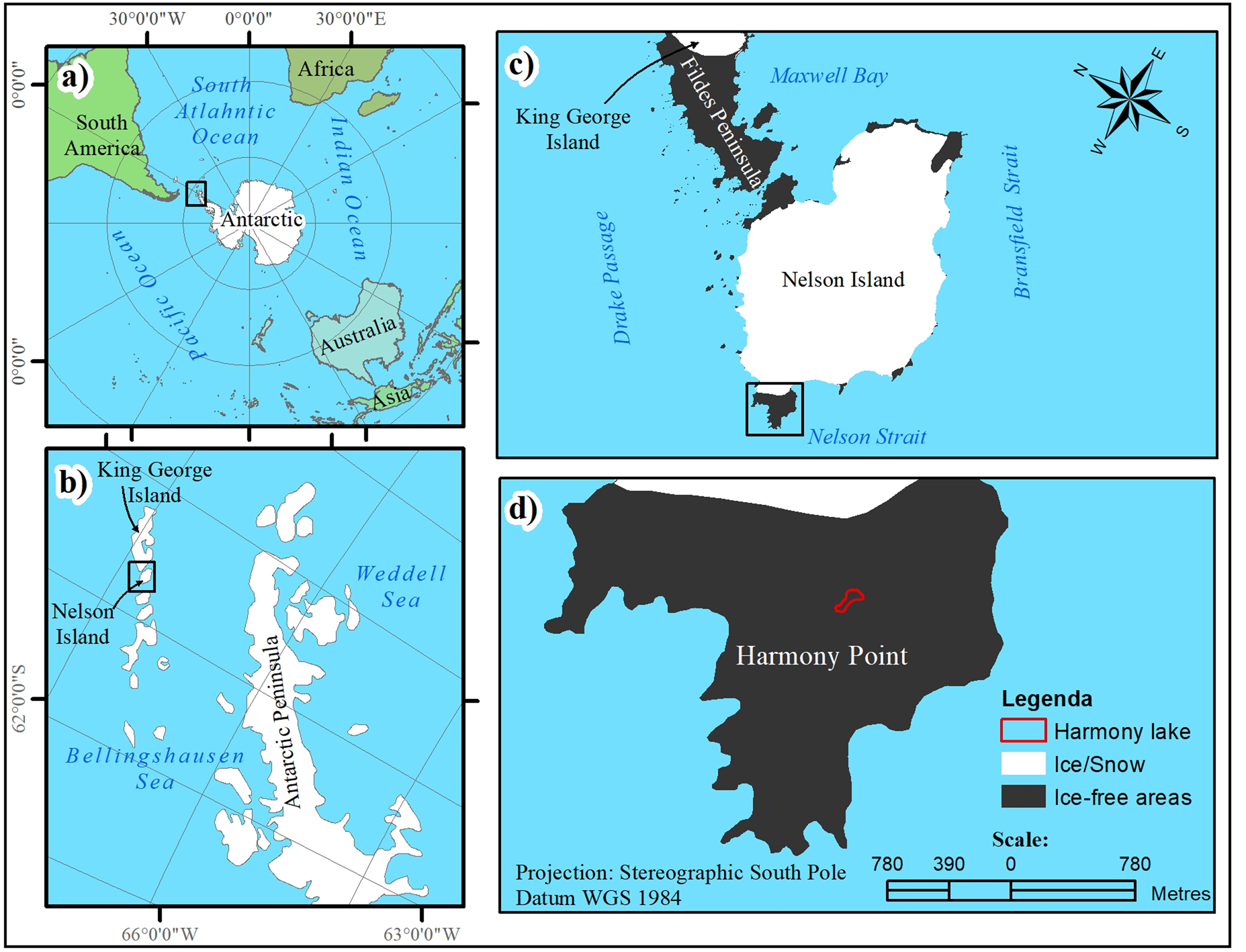
Fig. 1. Harmony Lake location map (west side of Nelson Island). a. Location of South Shetlands Islands, b. Nelson Island, c. Harmony Point and d. Harmony Lake location (west side of Nelson Island).
In that specific region, the climate is of the tundra type (Köppen Reference Köppen1948), where there is an average air temperature of -2.8°C, strong winds and an average annual rainfall of 425 mm (King & Turner Reference King and Turner1997, Bañón et al. Reference Bañón, Justel, Velázquez and Quesada2013). In summer, there is a great production of water from defrosting and vegetation growth (Jiahong & Jiancheng Reference Jiahong and Jiancheng1994, Braun et al. Reference Braun, Saurer, Vogt, Simões and Goßmann2001, Øvstedal & Smith Reference Øvstedal and Smith2001, Christopherson & Birkeland Reference Christopherson and Birkeland2015), mainly of cryptogams, at an average temperature of 2°C.
The soils are generally young and hardly developed, with a prevalence of turbic cryosols (Rodrigues et al. Reference Rodrigues, Oliveira, Schaefer, Leite, Gauzzi, Bockheim and Putzke2019). The lakes are mostly endorheic, small and shallow and located in depressions caused by deglaciation, which is a typical pattern for ice-free areas in the South Shetland Islands, as has been described by Simonov (Reference Simonov1977) concerning the Fildes Peninsula in King George Island. A rich biota was found in this area, with emphasis on the animal presence, predominantly birds, which may deposit guano in shallow lakes or humid terrains (López-Martínez et al. Reference López-Martínez, Serrano, Schmid, Mink and Linés2012, Reference López-Martínez, Schmid, Serrano, Mink, Nieto and Guillaso2016, Rodrigues et al. Reference Rodrigues, Oliveira, Schaefer, Leite, Gauzzi, Bockheim and Putzke2019).
Data
The data used in the analyses were collected during field research carried out between 8 and 15 February 2019. During this period, even under unfavourable weather conditions, it was possible to collect information regarding the limnological and spectral variables at seven sampling stations, as described below.
The analysed limnological patterns were water transparency (Transp), air temperature (AirT), water temperature (WT), TSS, chlorophyll a (chl a), turbidity, hydrogenionic potential (pH) and electrical conductivity (EC). Spectral information was acquired from a field spectroradiometer and a Landsat 8 image (surface reflectance product) from 8 February 2019, accessed through the US Geological Survey (USGS) database (http://earthexplorer.usgs.gov/). In addition, photographic flights of a Sensefly eBee unmanned aerial vehicle (UAV) were also performed for auxiliary data acquisition, such as the size and shape of the studied lake. The depth of the lake was assessed using a measuring tape that was weighed down until it came into contact with the lake bed.
Limnological parameter definitions
The limnological patterns for WT and Transp were determined simultaneously through water sample collection for further laboratory evaluation. Transp was obtained using a white Secci disk (SD) 25 cm in diameter attached to a graduated rope that was submerged in water, and the value of the depth at which it disappeared was registered. AirT was obtained by employing a thermometer positioned above the water and then submerged up to 5 cm to check that temperature against the WT.
After the water sample collection, the material was filtered with the least possible exposure to light to inhibit photosynthesis, properly stored and frozen. The remaining water samples were stored in thermal boxes at ~4°C. The filters and the water samples remained in this condition until the completion of the analyses of TSS, chl a, turbidity, pH and EC in the laboratory of the Federal University of Santa Maria (UFSM).
Turbidity, pH and EC were measured with the aid of the following equipment, respectively: Horiba multiparameter probe model U-53, Akso Ak90 and Hanna HI 933000. For this procedure, 200 ml of water from each sampling point was placed into a cup, in which the sensors were submerged and turbidity, pH and EC readings were taken.
TSS was obtained from the initial drying of the cellulose filters (0.45 μm pores) for 24 h in a hothouse at 50°C to determine humidity loss. Sequentially, the filters were weighed on a Mettler Toledo AG 245 analytical scale (0.0001 g of accuracy) for initial weighing (iW). These filters were then used for the filtration of the 250 ml volume of each sample and dried once more, and then they underwent a final weighing (fW). Thereby, the TSS measurement is given by applying the Equation (1) (Rice & American Public Health Association Reference Rice2012b).
 $${\rm TSS\;}( {{\rm mg\;}{\rm l}^{{-}1}} ) = \displaystyle{{( {{\rm fW}-{\rm iW}} ) {\rm \;} \times {\rm \;}100} \over {{\rm Filtered\;volume\;}( {{\rm ml}} ) }}$$
To determine chl a concentrations, a 250 ml volume of each sample was used. Chl a identification was performed through the following steps: filtration was conducted with a Millipore AP 40 borosilicate glass microfiber filter (without resin) with 0.7 μm pores. After the filtration process, the filter was submerged in methanol (10 ml) for 24 h and maintained at 4°C. Subsequently, absorbance was measured according to the spectrophotometric method without acidification (without the determination of pheophytin) at wavelengths of 663 and 750 nm (Mackinney Reference Mackinney1941). Finally, the absorbance measurement results were inserted into Equation (2) to obtain the chl a concentrations (Rice & American Public Health Association Reference Rice2012a).
 $${\rm Chl\;}a\;( {{\rm mg\;}{\rm l}^{{-}1}} ) = \displaystyle{{{\rm Abs\;}( {663-750} ) {\rm \;} \times {\rm \;}12.63{\rm \;} \times {\rm \;}V_{\rm met\;} \times {\rm \;}1000} \over V}$$
where Abs is the absorbance measurement at 663–750 nm wavelengths; 12.63 is a constant; V met is the methanol volume (ml), 1000 is another constant and V is the sample volume (ml).
Field spectroradiometer and photogrammetric flight
Field spectral data were collected between local time 11:00 am and 2:00 pm through the use of the FieldSpec® hand-held spectroradiometer with an operational range between 325 and 1075 nm and a spectral resolution of 1 nm (https://www.malvernpanalytical.com/br/learn/knowledge-center/user-manuals/fieldspec-handheld-2-user-guide) using the following collection procedures:
1) The spectroradiometer was positioned at each sampling station, on the boat, at a 135° angle from the sun and a 40° inclination of the sensor concerning the nadir. Under such circumstances, the spectroradiometer was first pointed at a Spectralon® reference panel, which has a Lambertian surface, for reference reflectance acquisition (which must be very near 100%) (Mobley Reference Mobley1999).
2) Under the same above-mentioned conditions, the spectroradiometer was repositioned to be directed at the water, hence obtaining the water reflectance measurement at the sampling station.
It is important to highlight that, in field research, the wind is an important spectral information-degrading factor. Therefore, it is important to always operate in adequate climate conditions, such as a sunny day with little wind, so that the water surface is only slightly waved (Pereira Filho et al. Reference Pereira Filho, Barbosa and Novo2005). However, given the extreme weather conditions at the research site, it was not possible to ensure field measurements were obtained under ideal conditions, thus the complete description of data collection conditions is necessary to ensure the presence of such information in the results analysis.
To contextualize the circumstances for each sample acquisition, Table I describes the conditions of the sky, water and surroundings of each station according to the interpretation of the researcher. Wind direction and velocity (V) were measured through the use of a Garmin compass and GPS receiver and a digital thermo-hygro-anemometer-luxmeter (Instrutherm, Model THAL 300). Each station and its surroundings were also photographed to support the data interpretation.

In the aerophotogrammetric survey carried out with the UAV, a Canon Ixus 16 megapixel camera was used, with the ability to obtain 5309 × 4615 pixel photographs at the red (R), green (G) and NIR wavelengths. The flights were performed simultaneously with in situ spectral and limnological data collection. During the research, two flights were executed at a height of 535 m, which allowed pixels with a 10 cm spatial resolution and with 85% longitudinal and 70% latitudinal overlap between each photograph. A total of 357 ha was overflown under climatic conditions in which winds varied between 1.9 and 8.0 m.s-1.
Spectral data analysis and processing
Spectral data acquired with the spectroradiometer were processed using the ViewSpecPro software. Data organization included the following steps: 1) FieldSpec® hand-held spectroradiometer files were exported to a spreadsheet for analysis, 2) reflectance values were converted to remote sensing reflectance (Rsr) (Ilori et al. Reference Ilori, Pahlevan and Knudby2019), 3) spectral curves were produced and analysed and 4) the first spectral derivative values were produced and interpreted.
The spectral curve obtained at each sampling station underwent a simulation of bands using the spectral response function (SRF), available in the Environment for Visualizing Images (ENVI) software for different orbital sensors. The spectral interval was restricted from 400 to 900 nm wavelengths because of the spectral range identified in the field. The simulated sensors were: Operational Land Imager (OLI), High-Resolution Imager (HiRI), RapidEye Earth Imaging System (REIS), MultiSpectral Instrument (MSI), WorldView-110 (WV110) and WorldView-3 (WV3), respectively, on board the Landsat 8, Pleiades 1A and 1B, RapidEye, Sentinel-2, WorldView-2 and WorldView-3 satellites. Sensor band simulation was carried out to test the potential of these satellites for monitoring the lakes in the region using remote sensing.
The simulated spectra were compared with observations acquired on the water pixels. The pixels of the sampling stations from the Landsat 8 OLI image in terms of surface reflectance values (Collection-2 Level-2 Science Products (L2SP)) were obtained from the USGS database (Global Visualization Viewer; http://earthexplorer.usgs.gov) (Earth Resources Observation and Science (EROS) Center 2013). The reflectance data employed in the simulation of the OLI sensor bands were obtained on the same day of the satellite's passage (8 February 2019). The positional accuracy of the L2SP was considered satisfactory.
Results
General characteristics
The mapped lake had an area of 13,934.20 m2 and an average depth of 0.57 m. It is a shallow lake elongated in an east-west direction, where the greatest depths (1.3 m) are located in its central and western regions. Figure 2 illustrates the photographic (false-colour) flight area, the field sampling stations and the observed depths. All sampling stations presented similar limnological patterns. In Table II, the collection conditions and the results of the limnological analyses carried out at the seven sampling stations are presented.

Fig. 2. Sampling stations map. a. Location of sampling stations, b. flight area and c. depth data. HP = Harmony Point.
Table II. Limnological and collection condition data.

AirT = air temperature; EC = electrical conductivity; chl a = chlorophyll a; NTU = nephelometric turbidity unit; TSS = total suspended solids; V = velocity; WT = wind temperature.
Concerning turbidity, it was possible to observe that only sample 7 showed a value close to 1 nephelometric turbidity unit (NTU). All chl a measurements were close to zero, with the highest concentrations found at stations 1, 2, 6 and 7. All sampling stations revealed an absence of TSS. These results corroborate field findings and are consistent with Transp and depth data, which showed equal values at the sampling stations.
The lack of optically active characteristics in the water, demonstrated by the abovementioned data, indicates that the spectral pattern of each sampling station may be influenced by the benthic conditions and communities (Fig. 3) of the lake. This is because the main differences in spectral curves are the colour at the bottom of the lake or the presence of rocks or brown aquatic vegetation/soil. The reflectance at 705 nm being greater than that at 583 nm indicates the presence of solids and/or vegetation at the bottom of the lake, as observed at stations 1 and 6 (illustrated in Fig. 3).

Fig. 3. Spectral patterns of water in the sampling stations.
Field spectra at stations 1, 2 and 4 were collected under scattered clouds in the sky. However, there was no cloudiness at the moment of spectrum acquisition. In the spectrum of station 1, a higher reflectance value was found in the red region, which is a fact possibly linked to the hazel colour of the bottom of the lake, where there is brown vegetation and sediment. On the other hand, at stations 2 and 4, where the bottom is characterized by light grey or white rocks and soil, a distinct pattern was observed, as the highest reflectance value was in the region of the yellow wavelength (571 nm), followed by a smaller difference between the absorption peak at the 678 nm wavelength and the reflectance peak at the 709 nm wavelength. A similar spectral pattern was found at stations 3, 5 and 7. The opposite was observed at station 6, in which the referred to difference was greater and similar to that detected at station 1.
It is noteworthy that, although the luminosity conditions under which the spectroradiometer samples were obtained cause differences in the absolute values of the spectra, they maintained a similar pattern. This fact was observed in spectra obtained under conditions of partially cloudy or cloudy skies, as there was an increase in reflectance values across the entire range of the electromagnetic spectrum used.
According to the graphs illustrating the first derivative of the spectra collected at each sampling station (Fig. 4), stations 2, 4 and 7 show lower values compared to other sites, especially at 695 nm. Therefore, it is possible to separate the seven sampling stations into two groups: the first (stations 1, 3, 5 and 6) is characterized by a brown lake bottom with the presence of sediment and vegetation; and the second (stations 2, 4 and 7) has a greater quantity of light grey or white rocks and sediment.

Fig. 4. Graphs of the first derivative of the sampling station spectral behaviour.
Spectra simulation
In the simulated spectra for each orbital sensor under study (Fig. 5), based on field spectra data (Fig. 5a), all stations show a decrease in reflectance between the green and red wavelengths. However, the spectral intervals on the sensor bands better captured the differences characterizing the aforementioned station groups. It should also be noted that due to the spectral similarity between the simulated data of the Pleiades 1A and 1B sensors, as well as that of the WorldView-2 and -3 sensors, only the simulated data of the Pleiades 1A sensor (Fig. 5e) and the WorldView-2 sensor (Fig. 5f) are shown.

Fig. 5. Simulated spectra map for the sensors: a. field spectra, b. MultiSpectral Instrument (MSI), c. Operational Land Imager (OLI), d. RapidEye Earth Imaging System (REIS), e. High-Resolution Imager (HiRI) Pleiades 1A and f. WorldView-110 (WV110).
Considering the spectral range of the spectral bands from the Sentinel-2 (Fig. 5b) MSI sensor, it can be verified that the spectra of stations 2 and 7 have lower reflectances in the red and red edge 1 wavelengths than in the green wavelengths. To a lesser extent, it is also possible to observe this fact at the other sampling sites. The opposite is perceived only at station 4, at which this difference is minimal.
From the simulated spectra of the Pleiades 1A (Fig. 5e), RapidEye (Fig. 5d) and WorldView-2 (Fig. 5f) sensors, it is observed that all sensors have the potential to distinguish between the two spectral groups. However, the RapidEye and WorldView-2 sensors allow greater differentiation between the spectra for water that has vegetation at the bottom and the spectra for those that do not. This difference is more visible in the spectral curves of sampling stations 1, 3 and 6 due to the increase in reflectance values in the red edge region. The opposite was detected at station 2, in which vegetation is absent, and in all simulated spectra there was a significant decrease in the reflectance values of the green wavelengths. However, it was not possible to detect differences between the two groups of spectra concerning the simulated data from the OLI sensor.
From the analysis of the spectral response of surface reflectances obtained from the Landsat OLI image acquired on 8 February 2019, it was possible to compare the spectra simulated in the field with the original spectra of the image (Fig. 6). Thus, to detect the influences of the edges of the lake and of its depth, the area of the lake obtained by the UAV on 11 February 2019 and bathymetric data from 12 February 2019 were also considered.

Fig. 6. Comparison between the spectra from the Operational Land Imager (OLI) sensor image and the simulation from the hyperspectral field data (S-OLI): a. sampling station P1, b. sampling stations P2 and P5, c. sampling stations P3 and P6, d. sampling station P4, e. sampling station P7 and f. location of sampling stations in the OLI image.
The sampling sites 3, 6 and 7 presented similarities between the shapes of the simulated spectra and the original spectra of the image only in the bands with wavelengths centred on 480 nm blue, 560 nm green and 655 nm red (Fig. 6c & e). The pixel area in the OLI sensor image is 900 m2, and the pixels in which samples 3 and 6 were inserted had 878.44 m2 of water, without influence from the lake edges, accounting for 97.6% of the pixels. It should also be considered that these samples were at a shallow depth of 0.6 m. Nonetheless, the pixels in station 7 represent 86.7% water, although inserted at a different depth (1.02 m), which may have led to a greater similarity between the simulated data and that of the image, especially if the absence of OACs in the studied lake is considered.
In addition, it is important to highlight the significant interference of depth and the edges of the lake at stations 1 (89.5% water), 2 and 5 (96.8% water) and 4 (96% water), all with average depths of 0.6 m. At these stations, there was considerable inconsistency between the simulated and field curves in the coastal aerosol and NIR bands. These analyses indicate that the spectra obtained from the image pixels at each sampling station present interference from the edges of the lake, as well as from the average depth of the pixel area of the OLI sensor image.
Discussion
Limnological behaviour
Most freshwater lakes found in ice-free areas in Antarctica are classified as ultra-oligotrophic because of the low levels of chlorophyll (Hansson et al. Reference Hansson, Dartnall, Ellis-Evans, MacAlister and Tranvik1996, Vinocur & Unrein Reference Vinocur and Unrein2000, Cremer et al. Reference Cremer, Gore, Hultzsch, Melles and Wagner2004, Toro et al. Reference Toro, Camacho, Rochera, Rico, Bañón, Fernández-Valiente and Marco2007, Lizotte Reference Lizotte, Vincent and Laybourn-Parry2008, Tanabe et al. Reference Tanabe, Yasui, Osono, Uchida, Kudoh and Yamamuro2017). This may be connected to the annual low levels of photosynthetically active radiation and ice cover that attenuate the light in the water column during winter in conjunction with the lack of any significant input of inorganic nutrients (Laybourn-Parry Reference Laybourn-Parry2002).
The low trophic levels of freshwater lakes in Antarctica are due to the dispersed distribution of habitats because of the extreme weather conditions and the high level of isolation around the continent (Cantonati et al. Reference Cantonati, Poikane, Pringle, Stevens, Turak, Heino and Richardson2020). However, on some Antarctic riverbeds, there are abundant nutrients such as dissolved inorganic nitrogen and phosphate (Tanabe et al. Reference Tanabe, Yasui, Osono, Uchida, Kudoh and Yamamuro2017), which confirms the existence of rich phytobenthic and endemic communities in some lakes in Antarctica (Toro et al. Reference Toro, Camacho, Rochera, Rico, Bañón, Fernández-Valiente and Marco2007, Nakai et al. Reference Nakai, Imura, Naganuma and Castro-Sowinski2019, Cantonati et al. Reference Cantonati, Poikane, Pringle, Stevens, Turak, Heino and Richardson2020).
The studied lake presented an average depth of 0.68 m, EC of 129 μS cm-1, pH 6.65 and WT of 4.28°C during the collection period in February 2019. A distinction was observed in the Terrasovoje and Radok lakes in Amery Oasis, East Antarctica, in which the average depths are much greater at 31 and 362 m, alkaline pH (between 7.3 and 8.2) and moderate conductivity (Cremer et al. Reference Cremer, Gore, Hultzsch, Melles and Wagner2004).
In lakes found in the ice-free areas of Skarvsnes and Langhovde in Lützov Holm Bay, East Antarctica, chl a concentrations were 0,5 μg l-1 at depths < 5 m and increased from this specific measurement until 9 m, reaching 14 μg l-1 (Kimura et al. Reference Kimura, Ban, Imura, Kudoh and Matsuzaki2010). In those lakes, changes in temperature and pH in the water column were also identified. Due to the low depth values found at HL, this observation was not identified at the study site. However, it is important to remark that similar pH and chl a values were also detected on the surface of the lake.
On Bayers Peninsula, Livingston Island, very low chl a concentrations were found, ranging from 0.03 to 0.31 μg l-1 at 1 m deep and from 0.09 to 0.18 μg l-1 close to the bottom of the lake (Rochera et al. Reference Rochera, Quesada, Toro, Rico and Camacho2017). However, lakes close to the sea had EC values > 100 μS cm-1 and high chl a values (between 17.0 and 40.5 μg l-1) due to the influences of the sea and of animal waste (Toro et al. Reference Toro, Camacho, Rochera, Rico, Bañón, Fernández-Valiente and Marco2007). These values are similar to conditions in lakes on South Georgia (Hansson et al. Reference Hansson, Dartnall, Ellis-Evans, MacAlister and Tranvik1996). These results corroborate those found in the present study, as the studied lake is located close to the sea, although it does not show any influence of animal waste, presenting chl a values < 2.5 μg l-1.
The lakes located on Poter Peninsula, King George Island, were divided by Vinocur & Unrein (Reference Vinocur and Unrein2000) into five groups. The fifth group appears to have low concentrations of nutrients, TSS and chlorophyll, so the data found classify HL as being in this group. Additionally, it is possible to verify that these characteristics are similar to those of stable and ancient lake surfaces located near the coast at high altitudes. Such lakes have maximum depths of 1.5 m, similar to those located in Ulu Peninsula, James Ross Island (Nedbalová et al. Reference Nedbalová, Nývlt, Kopáček, Šobr and Elster2013).
Water spectral behaviour
Reflectance peaks at the wavelengths near 710 nm are associated with the presence of chl a in water (Kutser et al. Reference Kutser, Paavel, Verpoorter, Ligi, Soomets, Toming and Casal2016). However, the absence of OACs in HL connected to the increase in reflectance values from the green wavelengths may be attributed to the spectral response of the bottom of the lake (Dierssen & Smith Reference Dierssen and Smith2000, Zeng et al. Reference Zeng, Zeng, Fischer and Xu2017), which has a maximum depth of 1.3 m and some reflectance peaks at the 710 and 800 nm wavelengths in sample spectra 1, 3 and 6, and whose bottom has vegetation. Furthermore, Ciotti et al. (Reference Ciotti, Lewis and Cullen2002) emphasize that in water bodies without those influences, such as in the oceans near the study site, a decrease in reflectances from wavelengths > 600 nm through absorption by pure water is expected.
The use of derivative analysis removes the reflectance signal from the pure water surface, highlighting some characteristics of chl a and TSS presence (Chen et al. Reference Chen, Curran and Hansom1992, Goodin et al. Reference Goodin, Han, Fraser, Rundquist, Stebbins and Schalles1993, Han & Rundquist Reference Han and Rundquist1997, Tsai & Philpot Reference Tsai and Philpot1998). Hence, chl a presence features around 690.7 nm in the first-derivative graphs (Fig. 4), which show similar behaviour to that provided by Han & Rundquist (Reference Han and Rundquist1997) and reinforce the lake bottom response presence in the spectra collected in HL. Accordingly, Tanabe et al. (Reference Tanabe, Ohtani, Kasamatsu, Fukuchi and Kudoh2010) report that elevated Transp allows 45–60% of photosynthetically active radiation (from 400 to 700 nm wavelengths) to reach oligotrophic freshwater lake bottoms, with depths up to 2.5 m in East Antarctica, and this enables moss field vegetal development at the bottom of these lakes.
Aiming at optimizing the environmental monitoring of aquatic compartments, Eleveld et al. (Reference Eleveld, Ruescas, Hommersom, Moore, Peters and Brockmann2017) used water spectral differences in various regions around the world to develop a spectral classification system based on the optical water type concept. However, it is important to observe that in the classification of these patterns, lakes such as HL are not considered, because of their low depth and organic and inorganic matter concentrations.
Yet water spectral reflectance is controlled by factors such as turbidity, depth, chlorophyll concentration and substrates in the water (Lyzenga Reference Lyzenga1978, Novo et al. Reference Novo, Hansom and Curran1989, Gitelson Reference Gitelson1992, Maritorena et al. Reference Maritorena, Morel and Gentili1994, Liew et al. Reference Liew, Choo, Lau, Chan and Dang2019). The absence of some of these organic and inorganic elements in the water column, such as in HL, enables features from the subsurface of the lake to be observed, where organic substrates show high reflectance at the wavelengths > 700 nm and, depending on the characteristics of the benthic communities of the lake, different wavelengths in this region may be more adequate for water depth and substrate type discrimination (Gilvear et al. Reference Gilvear, Hunter and Higgins2007)
Spectra simulation of orbital sensors
From field spectral data, Gilvear et al. (Reference Gilvear, Hunter and Higgins2007) simulated the efficiency of the sensors Airborne Thematic Mapper (ATM), IKONOS and Quickbird for mapping the substrate in Forth Estuary, Scotland. Overall, the authors indicate that the best results were obtained at the visible and NIR wavelengths near all simulated sensors for water depths up to 1 m. Distinctively, in the deeper water column (2–5 m), Kutser et al. (Reference Kutser, Vahtmäe and Martin2006) identified that the spectral range corresponding to the green area was the most effective for mapping algae cover in coastal environments from simulations of the spectra of the multispectral sensors Landsat, IKONOS and MERIS.
The simulation of bands in the OLI and Enhanced Thematic Mapper (ETM+) sensors from Hyperion hyperspectral images allowed for the identification of the superiority of OLI for identifying chl a and TSS concentrations and coloured dissolved organic matter (CDOM) (Pahlevan & Schott Reference Pahlevan and Schott2013). A similar result is seen for the reflectances directly obtained from images of the abovementioned sensors (Olmanson et al. Reference Olmanson, Brezonik, Finlay and Bauer2016), although the authors indicate that more studies are necessary to determine the superiority of OLI compared to ETM+ regarding Transp measurement in oligotrophic lakes.
When comparing the simulated spectral bands based on in situ spectra from OLI and MSI, Jorge et al. (Reference Jorge, Barbosa, Carvalho, Affonso, Lobo and Novo2017) found that the OLI sensor bands performed better at identifying TSS concentration, while the MSI sensor bands were more suitable for the detection of chl a, since the size and shape of the lake allow for the occurrence of water pixels without interference from other targets in the image. In addition, Kutser et al. (Reference Kutser, Paavel, Verpoorter, Ligi, Soomets, Toming and Casal2016) consider bands 5 (705 nm) and 7 (783 nm) of the MSI sensor to be the most appropriate for chl a identification, with band 7 being more indicated in the case of black lakes in which CDOM absorption can still affect the reflectance values in the 705 nm region.
In the present study, reflectance peaks in the yellow (571 nm) and red edge (678 and 709 nm) bands are reported, to which the presence or absence of elements such as clear rocks, soil and vegetation are attributed. A similar fact is determined by Gilvear et al. (Reference Gilvear, Hunter and Higgins2007), whose research results show distinct reflectances at the wavelengths between 575 and 625 nm and in the peaks centred at 650, 710 and 810 nm, which are inferred to be due to depth and substrate differences. In addition, it is important to stress that Kutser et al. (Reference Kutser, Vahtmäe and Martin2006) mention the influence of elements such as sand and vegetation in the water spectral response as a consequence of the high reflectance in the infrared near wavelengths.
It is important to emphasize that in the results generated from the band simulations obtained in the present study and from the works of Gilvear et al. (Reference Gilvear, Hunter and Higgins2007) and Kutser et al. (Reference Kutser, Vahtmäe and Martin2006), the influence of the atmosphere is disregarded and it is assumed that the data in situ do not have errors inherent to wind and solar angles (Jorge et al. Reference Jorge, Barbosa, Carvalho, Affonso, Lobo and Novo2017). Facts such as these, coupled with the absence of pixels of pure water and at reduced depth, may be the reason for the differences between simulated and real data from the OLI sensor shown in Fig. 6, as well as the identification of sensors that are more adequate for distinguishing the spectra acquired in the field, with more wavelengths located in the red and infrared regions.
Conclusions
In HL, chl a values < 3 μg l-1 were found in addition to turbidity and TSS values very close to 0. Transp reached values equal to the depth of each sampling station, a result that indicates the ultra-oligotrophic/oligotrophic nature of the lake at issue and the absence of OACs in this aquatic environment.
The spectral pattern of each sampling station, such as its low average depth (1.3 m), emphasizes the notion that the spectral properties of the lake are influenced by its benthic properties. This is evidenced by the reflectance values at 583 nm being lower than those at 705 nm where there is a presence of sediment and/or vegetation (as is shown in stations 1 and 6). Chiefly, it is possible to separate the seven sampling stations into two groups: the first group is influenced by brown lake bottoms due to the presence of soil and vegetation, as in stations 1, 3, 5 and 6; and the second group has a greater quantity of light grey or white rocks and soil, as in stations 2, 4 and 7.
Regarding the comparison between the simulated spectra shapes and the OLI sensor images, sampling stations 3, 6 and 7 showed similarities only in the bands with wavelengths centred at 480 nm (blue), 560 nm (green) and 655 nm (red). In such a context, the interference of the edges of the lake in the spectra from stations 1, 2, 4 and 5, all of these with an average depth of 0.6 m, becomes evident. It is also important to highlight the reduced number of pixels of pure water representing each sampling station, where only stations 3 and 6 showed less influence of the edges of the lake, with 878.44 m2 being the minimum water surface area identified over the image pixels.
Only the OLI sensor did not have the potential to clearly distinguish between the two spectral groups that were verified in the field. The best results for distinguishing the two spectral groups were obtained with the satellites Sentinel-2 and WorldView-2 and -3, as these satellites have a smaller widths and greater numbers of spectral bands in the yellow and red regions. Nonetheless, it is suggested to extend such research to larger and deeper lakes, as well as considering the acquisition of more sampling stations to enable a more comprehensive understanding of the spectral variability in Maritime Antarctic lakes.
Acknowledgements
The authors thank the National Institute of Science and Technology of the Cryosphere (INCT da Criosfera), Polar and Climate Center at the Federal University of Rio Grande do Sul, Terrantar Nucleus of the Federal University of Viçosa, the Department of Geosciences at the Federal University of Santa Maria, the Brazilian Navy, the Antarctic Support Station ESANTAR-RG and the National Council for Scientific and Technological Development (CNPq), process 310758/2016-5, 421743/2017-4, 408081/2013-9 and Coordination for the Improvement of Higher Level Personnel - Brazil (CAPES) - Code of Financing 001 for promoting the development of this research. The authors thank the two anonymous reviewers for their feedback.
Author contributions
CNR collected and analysed the measurements and authored the manuscript. UFB and WPF aided in the design, conception and approach and organized the field campaign. AMA and FLH aided in field trials. GK and JBJ contributed to the review of the article. All authors commented on and contributed to the manuscript.


