


Introduction
The Antarctic surface wind field is dominated by a persistent katabatic flow from the interior towards the coast. The topography plays the dominant role on the surface wind direction and wind speed (e.g. Parish Reference Parish1984). These drainage currents are illustrated in Parish & Bromwich (Reference Parish and Bromwich1987) showing distinctive major confluence zones, especially in East Antarctica. Terrain-induced pressure gradients result from temperature inversions over sloping terrain, which shape the near-surface wind field of Antarctica together with the Coriolis force and friction. Confluence zones, formed by valleys and ridges, the steep topography gradients near the Antarctic coast and the thinning of the inversion layer towards the coastal rim are accountable for strong coastal katabatic winds. Cyclic discharging periods of interior cold air pools lead to time-dependent katabatic surge events at coastal stations in which the wind speed reaches large magnitudes (e.g. Parish Reference Parish1984). Due to the Coriolis deflection, katabatic wind directions over the coastal slope are deflected between 10° and 50° from the fall line to the west, whereas in the interior, with more gentle topography, the deviation angle lies between 40° and 60° to the west (e.g. Parish Reference Parish1984). The high directional constancy of the surface winds is remarkable for most parts of the Antarctic and has been stated in several studies previously (e.g. Parish Reference Parish1984, Adolphs & Wendler Reference Adolphs and Wendler1995, Van den Broeke et al. Reference Van den Broeke, van de Wal and Wild1997).
Antarctic boundary layer winds are mainly a result of two pressure gradient forcing (PGF) components (e.g. Ball Reference Ball1956, Heinemann & Klein Reference Heinemann and Klein2002, Parish & Cassano Reference Parish and Cassano2003): i) the katabatic force (KF), which contains the forcing from a temperature inversion over sloping terrain, and ii) the synoptic force (SF), which is the superimposed PGF in the free atmosphere above the inversion layer. PGF can be summarized as:
 $$ PGF = {\rm{ - }}\frac{{\rm{1}}}{{\rm{\rho }}}\nabla P\,{\rm{ - }}\,g\frac{{{\rDelta}{{{\rm{\theta }}}_m}}}{{{{{\rm{\theta }}}_m}}}\nabla {{z}_s} = \,SF + \,KF, \eqno\rm$$
the first term describes the SF, where ρ is the air density and ∇P the two-dimensional pressure gradient of the free atmosphere above the inversion layer. In the second term, KF is defined by the gravitational acceleration (g), the inversion strength (potential temperature deficit in the katabatic layer; Δθm ), the mean potential temperature in the katabatic layer (θm ) and the two-dimensional terrain slope gradient (∇zs ). Terms resulting from inhomogeneities of the height of the katabatic wind layer and inversion strength are smaller by an order of magnitude and hence are neglected here. Parish & Cassano (Reference Parish and Cassano2001) concluded on the basis of NCEP-NCAR (National Centers for Environmental Prediction, National Center for Atmospheric Research) global reanalysis that both forcing terms are strongly shaped by the terrain gradient. Therefore, it is inappropriate to classify downslope winds as purely katabatic. Several authors in the past have examined the surface wind field of the Antarctic and Greenland, the northern counterpart, by distinguishing between KF and SF either on an observational approach (e.g. Heinemann Reference Heinemann1999, Renfrew & Anderson Reference Renfrew and Anderson2002) or by using numerical models on different horizontal scales (e.g. Parish & Cassano Reference Parish and Cassano2001, Reference Parish and Cassano2003, Heinemann & Klein Reference Heinemann and Klein2002, Van den Broeke & Van Lipzig Reference Van den Broeke and van Lipzig2003).
Parish (Reference Parish1984) carried out numerical simulations with a three-dimensional, hydrostatic, primitive equation model and stated that synoptic-scale forcing is only of secondary importance in shaping the drainage currents in the Antarctic. He attributed the primary forcing to the terrain-forced acceleration which shapes the patterns of katabatic flow. More than one and a half decades later Parish & Cassano (Reference Parish and Cassano2001) noted that the SF plays a more significant role than assumed, particularly for explaining the persistence of the summertime Antarctic boundary layer winds when surface radiative cooling and surface inversion strength are small compared to the winter season. Results of an aircraft-based study by Heinemann (Reference Heinemann1999) over the Greenland ice sheet in April/May 1997 have shown that the KF is the main driving mechanism for the near-surface flow, but a substantial SF was found as well. A comprehensive observation study of the surface climatology was carried out by Renfrew & Anderson (Reference Renfrew and Anderson2002) for the wind regime in Coats Land at the eastern Weddell Sea coast. They concluded that the flow is primarily driven by KF in less than 50% of the time, although in terms of wind characteristics the wind regime appears katabatic most of the time (60–70%). A similar conclusion was made by Parish & Cassano (Reference Parish and Cassano2003) for idealized surface characteristics of the Antarctic continent and a variety of synoptic constellations based on their model simulations. They showed that wind fields caused by katabatic processes cannot be definitively distinguished from other wind fields forced through synoptic conditions, and that wind direction alone is insufficient to identify KF. They concluded that the role of the katabatic flow over the Antarctic continent might be overemphasized.
Under favourable conditions Antarctic boundary layer winds can reduce the sea ice cover near the Antarctic coastal rim by pushing the adjacent sea ice offshore from the coastline or the fast-ice edge (e.g. Adolphs & Wendler Reference Adolphs and Wendler1995, Barber & Massom Reference Barber and Massom2007). In general, strong offshore winds are necessary for an initialization of such a coastal latent heat polynya. Polynyas are defined as recurring areas of open water or thin ice that are surrounded by thick ice and where thick ice would be expected due to the atmospheric conditions. Their recurrences are locally fixed but vary in time. A polynya event can persist for several hours or several weeks depending on the atmospheric conditions. Due to the decreased sea ice cover, heat flux from the ocean to the atmosphere is significantly enhanced compared to the surrounding sea ice pack. This leads to a weakening of the generally stably stratified boundary layer or even to the development of an internal convective boundary layer (e.g. Heinemann Reference Heinemann2008). Although tidal effects and coastal ocean currents can contribute to polynya formation, it is generally accepted that atmospheric forcing and, thus, offshore wind regimes are the major initiators for generating coastal polynyas. According to the three-year, satellite-based study by Markus et al. (Reference Markus, Kottmeier and Fahrbach1998) coastal polynyas in the Weddell Sea contribute between 2.5–5% to the sea ice volume produced in the Weddell Sea, comprising only a small area of 0.2% in the winter months (May–October). A long-term, model-based study by Haid & Timmermann (Reference Haid and Timmermann2013) reveals that coastal polynyas contribute 11% to the sea ice volume in the south-western Weddell Sea, whereas they cover only 0.6% during winter (May–September). Considering their small areal fraction in relation to their high ice production, their relevance for the Weddell Sea hydrography becomes evident. Enhanced brine rejection due to enhanced ice production within polynyas strongly modifies the shelf water formation and, therefore, the contribution to the Antarctic Bottom Water.
The aim of this paper is to study polynya dynamics in the south-eastern Weddell Sea area. The Weddell Sea in the southern Atlantic is one of the most dynamic polynya formation areas (Barber & Massom Reference Barber and Massom2007). Our focus is on the quantification of the relation to offshore wind regimes with respect to the two different forcing components KF and SF. We have implemented a high-resolution, non-hydrostatic regional weather prediction model for the Weddell Sea region (WSR) to address this issue (Fig. 1a & b). Polynya dynamics are studied for autumn and winter 2008 for the coastal region of Coats Land (see Fig. 1b for location). Coats Land is not known for extreme wind speeds, in contrast to other strong katabatic wind regions in the Antarctic, for example, Adélie Land or Terra Nova Bay, where several authors have proved polynya occurrence in relation to intense katabatic surge events (e.g. Adolphs & Wendler Reference Adolphs and Wendler1995). Nevertheless, Renfrew & Anderson (Reference Renfrew and Anderson2002) demonstrated that the wind regime of Coats Land is equally influenced by katabatic and synoptic systems, and that purely katabatic wind speeds reach a moderate strength with a mean katabatic wind speed of 7.5 m s-1 and maximum velocities of 15 m s-1.
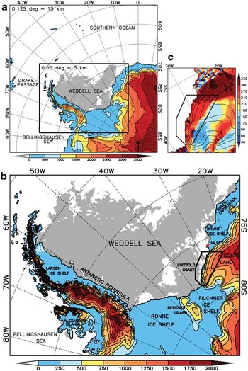
Fig. 1 a. COSMO 15 km model domain and sea ice cover (grey shading) from AMSR-E on 1 March 2008 (start of simulation period). Shaded colours and contours over land show the topography every 500 m. The black rectangle marks the nested COSMO 5 km model domain. b. COSMO 5 km model domain (20 pixels on each side are truncated) of the Weddell Sea region (WSR) and sea ice cover (grey shading). Shaded colours and contours over land show the topography every 250 m. The black polygon marks the study area. c. Slope direction in degrees (rotated model grid coordinates). For the atmospheric analysis all pixels within a slope direction between 180° and 360° were used within the polygon (yellow to dark red colours; an area of 29 660.5 km2). Wind directions in our analyses are transformed from the rotated model grid to geographic coordinates. Contour lines show the elevation every 250 m.
Data and methods
Design of the numerical simulations for the atmosphere
The non-hydrostatic, limited-area model of the Consortium for Small-scale Modelling (COSMO, version 4.11; Steppeler et al. Reference Steppeler, Doms, Schättler, Bitzer, Gassmann, Damrath and Gregoric2003) from the German Meteorological Service (Deutscher Wetterdienst, DWD) was adapted to the WSR for the autumn and winter period (March–August) 2008. We carried out daily forecast simulations with two mesh sizes (15 km and 5 km), considering a spin-up time of 6 hours (each model run covered 30 hours). Thus, 184 model runs were necessary for the chosen period of March–August 2008 for each horizontal resolution. For the first nesting step, runs with a grid size of 15 km were performed on a 300 x 300 grid point domain (Fig. 1a), which are driven by atmospheric fields from the global analysis of the global model GME provided by the DWD (Majewski et al. Reference Majewski, Liermann, Prohl, Ritter, Buchhold, Hanisch, Paul, Wergen and Baumgardner2002). In a second nesting step, the results of these simulations were used to drive the final simulations with a mesh size of 5 km and 450 × 350 grid points (Fig. 1b). Daily forecast simulations were carried out in order to keep the simulations close to reality. Moreover, each day a new sea ice mask was prescribed. Daily simulations were therefore necessary since up to now no adequate assimilation procedure for sea ice data exists for long-term simulations in COSMO. However, it should be noted that the results produced here may be useful for future long-term (coupled) model studies.
The model extends vertically up to 22 km with 42 sigma levels, ten of them are located beneath 500 m. The model equations are solved on an Arakawa-C grid. The sea ice cover was prescribed for each day by using the passive microwave satellite data of the Advanced Microwave Scanning Radiometer – Earth Observing System (AMSR-E; Spreen et al. Reference Spreen, Kaleschke and Heygster2008). For the treatment of the sea ice cover, the thermodynamic sea ice model of Schröder et al. (Reference Schröder, Heinemann and Willmes2011) was used. To distinguish between the polynya areas (POLA) and sea ice-covered ocean, areas with ice concentrations less than 70% were taken as POLA, a common threshold for polynya classification (e.g. Parmiggiani Reference Parmiggiani2006). Partial sea ice cover was not considered in a model grid box, the fraction was either 0% (open water) or 100%. The sea ice thickness was set at 1 m and a 10 cm snow layer was assumed above the sea ice. The albedo was set to 0.75 for snow-covered sea ice (slightly lower than the snow-covered inland ice, thus representing the subgrid-scale leads within the pack ice). The roughness length was prescribed above sea ice with a uniform value of 1 cm (Heinemann Reference Heinemann1997). Over water the roughness length was calculated by the Charnock formula. The water temperature within polynyas was set to -1.7°C (c. 0.15°C warmer than the freezing point of sea water). Ice growth within POLA was not enabled, assuming that newly produced sea ice would be advected away, like in a dynamic sea ice model and in reality. The land mask used here is the same as provided by the US National Snow and Ice Data Center (NSIDC). For a detailed and representative topographic description of Antarctica, we used the ETOPO1 Ice Surface dataset (Amante & Eakins Reference Amante and Eakins2009) in which the elevation of the ice shelves is already incorporated. From this dataset the roughness length of the surface was determined by calculating the slope-corrected orographic roughness length and by adding a constant roughness length value for snow cover of 1 mm (Van Lipzig et al. Reference Van Lipzig, King, Lachlan-Cope and van den Broeke2004a, Doms et al. Reference Doms, Förstner, Heise, Herzog, Mironov, Raschendorfer, Reinhardt, Ritter, Schrodin, Schulz and Vogel2011). The orographic roughness length results from the subgrid-scale variances. The mean terrain gradient of each pixel has to be subtracted for this procedure. Without that, an overestimated roughness length would be computed at grid points with strong terrain gradients.
The soil model of COSMO has eight soil layers (down to 14.58 m) and allows for an additional snow layer on top of the soil, which varies with precipitation and sublimation. For simplicity, we assumed the soil column as complete snow (instead of land ice) in the whole model region (ice sheet and ice shelves), except the southern tip of South America in the COSMO 15 km domain. Therefore, we modified the soil properties of the model and assumed a heat conductivity for snow of 0.3 W m-1 K-1 in the whole soil column, which corresponds to a snow density of 350 kg m-3. The albedo for inland ice and snow was set to 0.8. The initial fields for the snow properties were taken from the GME analyses, but it turned out that the depth of the snow cover of GME was unrealistically large. Therefore, initial snow cover was truncated to 0.06 m depth for the snow cover heat transfer. When we assumed the preset maximum depth of 1.5 m for snow cover heat transfer in COSMO (snow cover obtained from GME was several metres), the response of the surface temperature to atmospheric changes was very poor (e.g. weak daily cycle) through the damping effect of the top snow layer (see also Wacker et al. Reference Wacker, Ries and Schättler2009).
For the surface layer flux the parameterization of momentum, heat and moisture fluxes (Doms et al. Reference Doms, Förstner, Heise, Herzog, Mironov, Raschendorfer, Reinhardt, Ritter, Schrodin, Schulz and Vogel2011) is based on the similarity theory of Louis (Reference Louis1979). For the turbulence parameterization in the atmospheric boundary layer a prognostic turbulent kinetic energy closure at level 2.5 (based on Mellor & Yamada Reference Mellor and Yamada1982) including effects from subgrid-scale condensation and from subgrid thermal circulations is used (Doms et al. Reference Doms, Förstner, Heise, Herzog, Mironov, Raschendorfer, Reinhardt, Ritter, Schrodin, Schulz and Vogel2011). This setting is comparable to the configuration of the non-hydrostatic, high-resolution (35–3500 m) model simulations by, for example, Renfrew (Reference Renfrew2004) and Yu et al. (Reference Yu, Cai, King and Renfrew2005), who carried out idealized simulations using the Regional Atmospheric Modeling System (RAMS) to study katabatic flow dynamics over Coats Land. In previous studies different hydrostatic and non-hydrostatic models have been applied for Antarctic regions with different horizontal resolution, surface and boundary layer parameterizations (e.g. Heinemann Reference Heinemann1997, Van den Broeke et al. Reference Van den Broeke, van de Wal and Wild1997, Van Lipzig et al. Reference Van Lipzig, King, Lachlan-Cope and van den Broeke2004a, Reference Van Lipzig, Turner, Colwell and van den Broeke2004b). Cassano et al. (Reference Cassano, Parish and King2001) compared a number of widely used surface flux parameterizations used in numerical models with in situ measurements at Halley station (75.58°S, 26.57°W; see Fig. 1b for location) and stated that many of them underestimate the downward sensible heat flux under stably stratified conditions. King et al. (Reference King, Connolley and Derbyshire2001) tested four surface flux and boundary-layer flux parameterization schemes in the atmosphere-only version of the Unified Climate Model developed at the Hadley Centre of the Met Office (HadAM2) and suggested that the Louis scheme is appropriate for turbulent fluxes under stably stratified conditions. Luijting (Reference Luijting2009) carried out high-resolution numerical simulations using the UK Met Office Unified Model (MetUM) and examined the sensitivity of the model to the vertical resolution, the boundary layer parameterization, the stability functions and the roughness length. She found out that in all model simulations the katabatic layer was too deep and the surface wind was underestimated compared to observational data. Wacker et al. (Reference Wacker, Ries and Schättler2009) used a previous version of the COSMO model to study precipitation variability over Dronning Maud Land, Antarctica. They noticed that the COSMO model is able to reproduce the gross atmospheric features of the Antarctic atmosphere, but a warm bias in the lower troposphere and a weak daily cycle of the 2 m air temperature were apparent. The authors traced these deficiencies back to the treatment of soil and snow processes, as well as the simple assumption of sea ice conditions in the standard model configuration. As discussed above, we solved this deficiency in our implementation of the model.
Configuration of the sea ice–ocean model
The coupled Finite Element Sea ice–Ocean Model (FESOM; Timmermann et al. Reference Timmermann, Danilov, Schröter, Böning, Sidorenko and Rollenhagen2009) of the Alfred Wegener Institute, Helmholtz Centre for Polar and Marine Research was adapted for the WSR. The horizontal resolution at the coastal rim in the Weddell Sea was increased up to 3 km. Atmospheric forcing was provided by the results of our high-resolution simulations with 5 km grid size (Fig. 1b). The atmospheric variables of mean sea level pressure, 10 m wind speed, 2 m air temperature, 2 m dew point temperature, cloud cover and precipitation were provided every hour. A detailed description of the model can be found in Haid & Timmermann (Reference Haid and Timmermann2013).
Derivation of boundary layer conditions and polynya area
In our analysis, we determine the height of the stable boundary (katabatic wind) layer by using a threshold of the vertical potential temperature gradient, similar to Heinemann (Reference Heinemann1999). In a first step, we applied a threshold of the vertical potential temperature gradient of 0.01 K m-1 (Yu et al. Reference Yu, Cai, King and Renfrew2005), starting at the lowest model layer (c. 10 m above ground). In case of neutral conditions close to the surface due to strong mixing by intense katabatic winds, several inversions would be disregarded. In this instance we started a second detection from the basis on the fourth model layer (c. 100 m above ground). As an upper boundary the tenth model layer (c. 480 m above ground) was defined for the detection procedure, since the analysis focuses on regions with a stable katabatic wind layer over sloping terrain, and hence, inversion heights which do not exceed 500 m (Heinemann & Klein Reference Heinemann and Klein2002). In contrast, the atmosphere above the Brunt Ice Shelf (BIS, see location in Fig. 1b) is stably stratified up to at least 2000 m throughout the whole year (King Reference King1989). Using this detection method, the thickness of the inversion layer and the potential temperature deficit within this layer was calculated. While the inversion layer deduced from temperature inversion can be several hundred metres thick above the slope, the highest katabatic wind speeds occur in the lowest 100 m above ground (Renfrew & Anderson Reference Renfrew and Anderson2006). The synoptic pressure gradient was calculated on the thirteenth model layer (c. 970 m above ground). At this height, we assume SF conditions being unaffected by surface conditions (Heinemann & Klein Reference Heinemann and Klein2002).
Time series of the POLA in the study area are derived from two different remote sensing techniques and from the sea ice–ocean model FESOM. As mentioned earlier, POLA from AMSR-E satellite data is deduced using a threshold of 70% of the sea ice fraction. The second remote sensing dataset consists of thin-ice retrievals using brightness temperatures from the MODerate-resolution Imaging Spectroradiometer (MODIS) satellite (Adams et al. Reference Adams, Willmes, Schröder, Heinemann, Bauer and Krumpen2013). POLA is calculated by using a threshold for sea ice thickness of 20 cm (Adams et al. Reference Adams, Willmes, Schröder, Heinemann, Bauer and Krumpen2013). The passive microwave data (AMSR-E) provides complete coverage of sea ice concentrations every day for our study area with a horizontal resolution of 6.25 km. Whereas the thermal infrared MODIS satellite data has a much finer resolution of c. 1 km, but daily assessment is not assured since cloud coverage may prevent attainment of information on the sea ice–ocean surface. For that reason, POLA from MODIS is used for verification only if the coverage of the daily composite is larger than 50% over the sea ice–ocean area within the polygon in Fig. 1c. To take into account the missing areal coverage of the used residual scenes, POLA is increased according to the percentage of the missing area. POLA from the sea ice–ocean model FESOM is deduced by using the 70% threshold of the sea ice fraction and, in addition, the 20 cm threshold of the sea ice thickness, as it was done for the AMSR-E and MODIS satellite data.
Verification of the model simulations
The quality of our simulations is proofed by a comparison between observations and model results. Since no simultaneous measurements are available for our sloping study area of Coats Land, we use observations from the manned station Halley on the BIS, close to our study area (Fig. 1b). Observations from automatic weather stations (AWS) were also available for the simulation period on the Ronne Ice Shelf (Limbert AWS) and Larsen Ice Shelf. However, since these stations are maintained only once a year (Steve Colwell, British Antarctic Survey (BAS), personal communication 2012), the reliability, particularly of wind measurements, must be considered carefully. Wind measurements of AWS in polar regions are strongly prone to rime and snow cover in winter. Analyses of time series for the Limbert AWS (75.91°S, 59.26°W) and Larsen Ice Shelf AWS (67.01°S, 61.55°W) showed some deficiencies in wind speed records (not shown). In this instance, we decided to only use the Halley station, primarily due to the geographical proximity to our study area. At Halley, wind speed and direction are usually measured at 10 m above ground, but in 2008 an AWS was in operation due to restructuring measures and wind measurements were taken at 2 m above ground (Steve Colwell, BAS, personal communication 2012). To compare measured (2 m) and modelled (10 m) surface wind speed we extrapolated the AWS wind speed to 10 m assuming neutral stratification and a roughness length of 1 mm for snow-covered surfaces (resulting in a factor of 1.21). Statistical comparisons of the meteorological variables were carried out on an hourly basis for the whole simulation period. Table I shows the statistical comparisons between observations and model results for mean sea level pressure (mslp), 2 m air temperature (T2m), 10 m wind speed (ff10m), surface wind direction (dd) and directional constancy (dc). A good accuracy can be noticed for the simulation of the mslp with a small bias of 1.4 hPa and a correlation coefficient at 0.98. The standard deviations of modelled and observed mslp are close together. A correlation coefficient at 0.79 and a bias of 0.7 K is found for the T2m, while standard deviations are also close together. A bias of 0.6 m s-1 and a correlation coefficient at 0.8 is found for the ff10m, while the standard deviation of the observed ff10m is 1.2 m s-1 greater than the model data. A more easterly dd is found for the observed wind, but only a small bias of -3.7° exists. The dc is 7% smaller in the simulations.
Table I A statistical comparison (mean (
 $$--><$>{{{\overline{\bi X}}}}$$$
), bias (mod-obs), standard deviation (SD) and correlation coefficient (r)) of meteorological variables at Halley for the simulation period (on an hourly basis) between observations (obs) and model (mod) results: mean sea level pressure (mslp), 2 m air temperature (T2m), 10 m wind speed (ff10m), wind direction (dd) and directional constancy (dc).
$$--><$>{{{\overline{\bi X}}}}$$$
), bias (mod-obs), standard deviation (SD) and correlation coefficient (r)) of meteorological variables at Halley for the simulation period (on an hourly basis) between observations (obs) and model (mod) results: mean sea level pressure (mslp), 2 m air temperature (T2m), 10 m wind speed (ff10m), wind direction (dd) and directional constancy (dc).

Compared with the results of Wacker et al. (Reference Wacker, Ries and Schättler2009) who diagnosed a warm bias in the lower troposphere between model results and observations (model simulations were too warm), we can assume that the results of our improved model configuration (e.g. soil and snow treatment, sea ice model, prescribed sea ice cover and roughness length) are not affected by a warm bias in the lower troposphere. The high correlation coefficient of the T2m, the nearly equal standard deviations and the small bias of the hourly comparison indicate that the COSMO model can reproduce the variability of the T2m at Halley with a good accuracy. Also the measured surface wind speeds and directions are well-reproduced by the model (Table I).
To assess the upper air performance of the model we compared radiosonde ascents from Halley with our model results. For our study period (184 days), 100 radiosonde ascents are available from BAS, which are launched every day at around 11:00 UTC, if an ascent was done. Approximately 200–250 measurements are taken during an ascent in the lowest 2000 m above ground. Only 17 model levels in the lowest 2000 m are available for the comparison. Air temperature, wind speed and wind direction for three radiosonde ascents for the 19, 21 and 22 July are shown in Fig. 2. These dates were chosen with respect to our case study of the 21 July shown in the results. For the 20 July no radiosonde was available. It can be seen that in general the temperature and wind speed profiles of the lowest 2000 m are well-reproduced by the model. However, it is striking at all dates that in the lowest decametres the measured inversion strengths are much stronger than the ones of the simulations. At the same time, simulated near-surface wind speeds are apparently stronger than the measured ones (Fig. 2b & e). These overestimated near-surface wind speeds could lead to stronger turbulence in the surface layer of the model simulations and thus, a weakening of the surface inversion strength. Furthermore, it can be noticed that with decreasing wind speed the quality of model wind direction decreases (Fig. 2c & i).

Fig. 2 Radiosonde profiles (black dots) and profiles derived from model simulations (red dots) for the lower 2000 m (hagl = height above ground level) at Halley (see Fig. 1b for location). Air temperature (T), wind speed (ff) and wind direction (dd) are shown for three days (two days before, during and one day after the case study presented in Fig. 7).
Results
Mean katabatic wind dynamics of the Weddell Sea Region for March to August 2008
The mean wind field and boundary layer conditions for the autumn and winter period (March–August) 2008 are presented in Fig. 3. Over the large and flat Filchner–Ronne Ice Shelf (FRIS) in the south (see Fig. 1b for location) and over the sea ice-covered Weddell Sea (Fig. 3d), wind speeds do not exceed 6 m s-1 (Fig. 3a). At the west side and to the north of the Antarctic Peninsula (see Fig. 1b for location) higher wind speeds up to 10 m s-1 are simulated. The flow blocking of the Antarctic Peninsula is reflected by very low winds directly on its eastern flank (lower than 4 m s-1) and by stronger winds on the west side (up to 10 m s-1). A mean low pressure system over the Bellingshausen Sea (see Fig. 1b for location) leads to a north-easterly flow at the south-western part of the Antarctic Peninsula, which is channelled between the blocking Antarctic Peninsula and the adjacent Alexander Island in the west (see Fig. 1b for location). This fact is underlined by the high dc of the 10 m (surface) wind in Fig. 3b with values larger than 0.75 and even 0.9 in the centre of this channelling area. In the eastern WSR areas, high wind speeds are visible in the lower right corner of the model domain that is over the ice slopes towards the FRIS (Fig. 3a), where mean surface wind speeds up to 12 m s-1 are simulated. The dc exceeds 0.95 over a large area in this region (Fig. 3b). Furthermore, this area shows the highest values for the inversion strength (up to 15 K; Fig. 3d) over sloping terrain with a maximum mean inversion thickness of 450 m (Fig. 3c). Therefore, it can be assumed that KF is strong in this area and leads to strong winds with high dc. The second region in the eastern Weddell Sea with relatively high mean wind speeds is located at Coats Land. Wind speeds up to 10 m s-1 (Fig. 3a) and a dc between 0.5 and 0.9 (Fig. 3b) are present. Much weaker inversion strengths (up to 7 K) are present above Coats Land compared to the region south of the Filchner Ice Shelf (FIS). A further prominent feature is the well-developed trough along the eastern coast of the WSR which extends far to the south, almost to the FIS (Fig. 3a). It can be assumed that this trough has a significant influence on the wind field of the Riiser-Larsenisen (see Fig. 1b for location), the BIS and the slopes of Coats Land. At the west side of Berkner Island (see Fig. 1b for location) local katabatic winds can be seen, whereas on the east side the area of high dc over the flat FIS indicates the interaction of this coastal trough with the katabatic currents from the upslope terrain of the FIS. The high dc of enhanced offshore winds in the south-eastern part of the Antarctic Peninsula indicates the presence of a barrier wind system.

Fig. 3 a. Mean 10 m wind speed (colour-coded) in m s-1 and mean 10 m wind vectors (every eighth grid point) in m s-1 for March–August 2008. Contour lines over sea ice–ocean show the mean sea level pressure (interval = 1 hPa). b. Directional constancy (colour-coded) of the 10 m wind for March–August 2008 with mean 10 m wind vectors (every eighth grid point) in m s-1. c. Mean surface inversion height in m. d. Inversion strength in K. Thick to thin contour lines (180d, 160d, 80d, 0d) drawn over sea ice–ocean mark the sea ice cover (ic) in days (d) for our study period. Contour lines drawn over land represent the topography every 250 m.
Over the sea ice-covered, south-central Weddell Sea the inversion strength is relatively large (c. 10 K, Fig. 3d), and the inversion height is larger than the maximum detection height of c. 500 m (Fig. 3c, grey area). The inversion strength in this area changes according to the temporary extent of sea ice in the Weddell Sea. The inversion strength is most pronounced for areas with more than 180 days of sea ice coverage. At the coastline of the eastern Weddell Sea the inversion layer is disrupted (white areas in Fig. 3c & d), associated with the frequent polynya activity in this region and the accompanying formation of a convective boundary layer. Without polynya activity it can be assumed that the inversion strength would be stronger and more homogenously distributed. A further prominent result is the decrease of the inversion thickness and inversion strength at the foothills and over the lower part of the sloping terrain in the eastern WSR (Fig. 3c & d).
The forcing mechanisms and associated polynya dynamics at Coats Land
The mean acceleration forces for SF and KF, and number of polynya days are illustrated in Fig. 4 for the region of Coats Land. The SF component is distributed fairly homogeneously over the entire domain compared to KF and has its strongest values directly at the transition between the steep coastal slopes and the ocean/sea ice (Fig. 4a). A mean SF between 1 × 10⁻³ m s-2 and 1.5 × 10⁻³ m s-2 is present for almost the entire area. Slightly weaker values are evident over the FIS, and slightly larger values over the BIS and the northern slopes of Coats Land. While a large-scale northward orientation of the SF above the ocean/sea ice and the BIS is visible, the SF over Coats Land and particularly in our study area (polygon in Fig. 4) shows no directional preference for the SF pattern (vectors in Fig. 4a). In contrast, the KF pattern is strongly shaped by the topography and, therefore, has a more heterogeneous distribution over sloping terrain (Fig. 4b). In general, katabatic accelerations increase in the downslope direction because of increased terrain gradients towards the steep coastal slopes. By definition, the KF is always directed along the fall line, whereas the orientation of the SF can vary under consideration of synoptic pressure systems. As expected, the KF is close to zero over the ice shelves due to the relatively flat terrain.

Fig. 4 Mean (March–August) of a. the SF and b. the KF in 1 x 10⁻³ m s-2. Colour bar at the bottom is valid for the whole region of a. and over land in b. Mean acceleration vectors in 1 x 10⁻³ m s-2 (every third grid point). Colour bar at the right is valid for the shaded area over the sea ice–ocean in b. and shows the polynya days of the study period. Contour lines drawn over land show the topography every 250 m. The black polygon marks the study area.
Polynya days from March–August 2008 are shown in Fig. 4b. A polynya day is counted if the sea ice fraction falls below 70% in the daily available AMSR-E data. A high polynya frequency is found at the southerly edges of the BIS. With around 60–100 polynya days in these regions, the duration is twice that observed at the Luitpold Coast (see Fig. 1b for location). Therefore, our study area is located in the immediate vicinity of the BIS region with high polynya activity. Thus, a preconditioning of sea ice properties originating from the north-east could influence the polynya activity in the northern part of our study area. The same is valid for the south-western border and the adjacent sea ice conditions at the FIS with its different wind regime. This should be considered in further POLA analysis.
Time series of POLA, acceleration forces and surface wind speeds are shown in Fig. 5. The red and purple lines in Fig. 5a represent the POLA (previously mentioned thresholds applied) resulting from the global sea ice–ocean model FESOM with atmospheric forcing by the COSMO 5 km simulations. The black line and the dotted green line show the POLA from the two remote sensing datasets AMSR-E and MODIS, respectively. To identify polynya openings and follow polynya activity the most notable changes in POLA (AMSR-E POLA as reference) are indicated by the coloured bars, grey for polynya openings (O) and orange for closings (C). Only POLA clearly exceeding 500 km2 (black dashed line) within the period of an opening is considered. A polynya closing is defined by a decrease of POLA to the last value below 500 km2 with the absence of an immediate reopening. Under these conditions six opening events and five closing events can be identified (see Fig. 5a).

Fig. 5 Polynya area (POLA) and atmospheric variables as daily averages within the study area (polygon in Fig. 4b). a. POLA from AMSR-E data (using the 70% threshold of sea ice fraction, black line), from MODIS composites (using the thin-ice algorithm of Adams et al. (Reference Adams, Willmes, Schröder, Heinemann, Bauer and Krumpen2013) and a 20 cm threshold for sea ice thickness, green line with dots), and POLA simulated by the sea ice–ocean model FESOM forced with COSMO 5 km outputs (70% threshold for sea ice fraction, red line; sea ice thickness threshold of 20 cm, purple line). The dashed black line marks the area of 500 km2. b. Accelerations over sloping terrain (slope direction between 180° and 360°, see Fig. 1c): katabatic acceleration KF (blue; area weighted), total synoptic acceleration SF (solid red), SF component along the fall line (dotted red), slope-parallel SF component (dashed red) and PGF along the fall line (green; sum of KF and downslope SF component). c. Wind speeds over sloping terrain (slope direction between 180° and 360°, see Fig. 1c): 10 m wind speed (solid red line), 10 m wind component along the fall line (red dashed line), and the fall line component of the 10 m wind for grid points where a KF was detected (blue line, area weighted). The grey bars illustrate polynya openings and following polynya dynamics, whereas the orange bars highlight polynya closings (AMSR-E data as reference). The different openings and closings are named as O and C, respectively, using increasing numbers. The star indicates the date of the case study (Fig. 7).
Overall, time series of POLA derived from AMSR-E and MODIS agree well considering the different remote sensing methods and data sources. Most of the time POLA determined from MODIS are larger, but there are also periods when MODIS POLA are less than AMSR-E POLA (e.g. O6). The two main problems when getting the correct POLA from MODIS data are the spatial coverage of the daily composites and the errors in cloud detection over sea ice in winter. If the main polynya region in the MODIS composite is covered by clouds, an underestimation of POLA is unavoidable, even with the applied correction method. A false detection of clouds can strongly influence the MODIS thin-ice retrieval and, hence, influence the POLA signature. On the other hand, a main problem of AMSR-E data is the relatively coarse horizontal resolution (6.25 km). Small-scale polynyas are not resolvable with this resolution and, hence, the AMSR-E data tends to underestimate the POLA compared to the MODIS thin-ice thickness approach. In addition, thin ice-covered polynyas may be undetected by AMSR-E.
All six main polynya events are represented by both satellite datasets. For the FESOM simulations a general underestimate of POLA is found. Besides that, the applied threshold of 70% to the modelled sea ice fraction seems to be more suitable for polynya detection than the 20 cm sea ice thickness threshold. The polynya dynamics of O1/C1 and O5/C5 are qualitatively well reproduced by FESOM, but POLA is too small. While the small POLA maximum of O4 is simulated well, the relatively large events O2 and O6 are not captured by the FESOM simulation. The polynyas at Coats Land certainly belong to the small-scale ones within a very narrow band along the Luitpold Coast (see Figs 3d & 4b), which are difficult to simulate even with such a high resolution as used here in FESOM.
To identify the relationship between wind forcing and the different opening and closing periods we calculated the daily mean of SF, KF and surface wind speed within our study area using only land points which potentially influence the coastal area of Coats Land (defined by a slope direction between 180° and 360° in our study area, see Fig. 1c). The solid red line in Fig. 5b denotes the absolute value of SF. Since KF (blue line) is always directed along the fall line (downslope), the downslope component of the SF (dotted red line) is shown additionally to compare downslope acceleration of KF and SF. Positive values denote downslope (offshore) accelerations (north-easterly ‘slope-parallel’ geostrophic wind components) and negative values denote upslope (onshore) accelerations (south-westerly ‘slope-parallel’ geostrophic wind components). ‘Slope parallel’ is defined here for wind and pressure gradient components following lines of constant altitude of topography. In addition, the slope-parallel component of SF is illustrated by the dashed red line in Fig. 5b. Positive values of the slope-parallel SF component correspond to geostrophic downslope (offshore) wind components and negative values correspond to geostrophic upslope (onshore) wind components. The PGF (green line) is the sum of KF and the downslope SF, see Eq. (1). Since the area of KF can be less than the area of SF, due to missing katabatic conditions, KF is weighted by the sum of the katabatically influenced land points divided by the sum of the used land points (slope direction criteria) described before. Surface wind speed (solid red line) and the calculated downslope component of the surface wind (dashed red line) are displayed in Fig. 5c. The downslope component of the surface wind for grid points with katabatic conditions is shown by the blue line and is area-weighted like KF, if the KF area is less than the SF area.
Within the different opening and closing periods several interesting features are visible. It is striking that significant extremes in POLA (black curve in Fig. 5a; AMSR-E as reference) are associated with pronounced maxima of the different acceleration forces and their directional components (Fig. 5b). This can be clearly seen for the transition between O2 and C2 and during O5. Generally, there is a strong increase of KF during each initial phase of an opening period (O2–O5), except for O6 where the SF, and particularly the downslope SF, increase considerably, while the slope-parallel SF remains near zero. In contrast, strong decreases of KF are associated with polynya closings. Even in opening periods, intermediate decreases in POLA are linked to a temporary strong weakening of KF, best noticeable in O2 and O5. The phases of most pronounced KF are associated with a strong component of synoptic onshore acceleration (downslope SF is negative, thus leading to a south-westerly geostrophic wind component) and a positive slope-parallel SF (offshore geostrophic wind component). The correlation coefficient between KF and the slope-parallel SF is 0.59 for the study period and 0.7 for July. A negative correlation coefficient between KF and the downslope SF of -0.75 is found for the study period and of -0.9 for July. The rise of the correlation coefficients in July 2008 indicates that the opening phase O5 can be seen as the most interesting period for our study of katabatic wind and polynya dynamics, since strong connections between the directional components of SF and KF exist, and a high variability of POLA, wind speed and acceleration forces is present.
The findings for the downslope component of the surface wind (blue and dashed red line in Fig. 5c) are similar to those of KF. There is a rapid increase of the downslope component of the surface wind speed in the initial phase of opening periods and a rapid weakening in closing periods, indicating a refreezing of polynyas during the weakening of surface offshore wind components. With very few exceptions, the downslope components of the study area and the katabatically influenced study area show no large differences. This indicates that a flow in a downslope direction is nearly always of katabatic origin. The surface wind speed (solid red line in Fig. 5c) differs strongly from the downslope surface wind component. Temporary high surface winds are often mainly directed along the coast, which is when the downslope surface wind component is small. These periods with weak KF and enhanced SF are mainly a result of cyclonic activity associated with a pronounced onshore geostrophic wind component (slope-parallel SF is negative) and a north-easterly slope-parallel geostrophic wind component (downslope SF is positive) most of the time. This situation is typical during closing periods or periods without significant polynya activity (orange and white coded periods in Fig. 5). For three of the opening periods (O3, O4 and O5), the opening begins after a period of strong SF surface winds (strong SF in Fig. 5b and strong surface winds in Fig. 5c) when a decrease of the surface wind speed is followed by an increase of (katabatic) downslope wind components. The possible role of SF surface winds for preconditioning of the sea ice and facilitating subsequent polynya formation is discussed below.
The positive downslope SF implies a north-easterly geostrophic wind component (associated with a trough along the coast of the eastern WSR, see Fig. 3a) and unfavourable conditions for polynya openings at the Luitpold Coast. During these synoptic conditions, sea ice is transported alongside the Luitpold Coast and is pushed against the FRIS. In contrast, the downslope SF becomes negative during strong opening periods, clearly visible in the transition between O2/C2 and O5. These strong negative values of the downslope SF correspond to a strong south-westerly geostrophic wind component and hence, a large-scale north-easterly transport of sea ice is allowed for. The constellation of a strong downslope katabatic wind component, supported by a southerly geostrophic offshore wind represents favourable conditions for sea ice transport away from the Luitpold Coast and the development of large polynyas.
In the period between C4 and O5 (from mid to the end of June), a relatively strong KF signal can be seen, but there is only a very weak polynya signal in both remote sensing datasets. A reason for this could be the negative slope-parallel SF corresponding to an onshore geostrophic wind component in this period, while KF and the downslope SF behave similarly in O5. This results in relatively weak surface winds and downslope surface wind components even for strong KF. Although this constellation is rare, the weak wind conditions associated with low cloudiness (not shown) led to unusually cold conditions over the BIS. Observations of the T2m at Halley on the southern BIS, adjacent to Coats Land, show temperatures down to -50°C for that period (not shown), which are the lowest T2m measured in the period of our investigation in 2008 (typical T2m minima are between -30°C and -40°C). Furthermore, measured wind speeds do not exceed 5 m s-1 most of the time with wind directions between 200° and 300° (not shown). This indicates that extremely cold air from the FRIS is advected to the region of Coats Land. Our model reproduces these atmospheric conditions at Halley very well.
In conclusion, the analysis of time series of wind, POLA and forcing terms shows that changes in POLA are mainly steered by the downslope component of the surface wind. The correlation between the POLA day-to-day change and the downslope surface wind component reveals a correlation coefficient of 0.71 for the complete study period (Fig. 6a) and 0.84 for July. The downslope component of the surface wind is steered in turn by the PGF along the fall line with a correlation of 0.84 (Fig. 6b) and 0.86 for July. The KF term (see Eq. (1)) has a correlation with the downslope surface wind component of 0.63 for the whole study period and 0.8 for July. In contrast, the downslope SF term (see Eq. (1)) is negatively correlated with the downslope surface wind component (-0.11 for the whole period and -0.57 for July). This shows that a south-westerly geostrophic wind component is an important factor in times of increased downslope winds and thus polynya activity. Moreover, a high correlation of 0.79 for the whole period and 0.88 for July is also found between the downslope component of the surface wind and the slope-parallel SF. This underlines the importance of a suitable synoptic offshore component for katabatic wind dynamics. However, KF is much larger than the magnitude of the slope-parallel SF during polynya opening periods. Therefore, it can be concluded that the main part of the downslope surface wind speed is forced through katabatic acceleration. Regarding the mean surface wind speed over Coats Land it is clearly evident that the surface wind field is steered most of the time by the SF. A correlation of 0.79 for the whole period of investigation and 0.68 for July underlines this relation. Furthermore, the lower correlation coefficient in July indicates a weakening impact of the SF on the surface wind regime, while the correlation coefficient between the KF and the downslope surface wind component rises, in periods of strong POLA variability.

Fig. 6 a. Correlation between day-to-day change of POLA (AMSR-E) and 10 m wind speed along the fall line (dashed red line in Fig. 5c) for the study period. Considering only significant changes, day-to-day changes smaller than 300 km2 are neglected. b. Correlation between fall line 10 m wind speed (dashed red line in Fig. 5c) and fall line PGF (solid green line in Fig. 5b) for the study period.
Case study of a katabatic wind event and polynya formation
We will now present a case study of the most prominent POLA event in winter for 21 July 2008 (stars in Fig. 5). A MODIS infrared image for 1040 UTC 21 July 2008 is shown in Fig. 7a, corresponding model results are shown for 1100 UTC 21 July 2008 in Fig. 7b–e. Several interesting features can be discovered in the MODIS image. At the coast, the strong warm signature of a narrow polynya (probably covered by thin ice) can be seen. Over the sloping terrain of Coats Land a large green area indicates relatively warm temperatures, which is a typical katabatic wind signal. The surface temperature of the sloping terrain is increased due to the enhanced downslope wind speeds and the accompanied increased vertical mixing in the katabatic wind layer. The warm katabatic signature over the slopes is also present in our model results (Fig. 7c). In general, the warming signature ends in a convergence zone which is identified through a yellow thermal belt along the foothills of the sloping terrain in the MODIS scene. Several streaks of warm signatures are also visible over the BIS and the small area of fast ice at the Luitpold Coast. They indicate that air of katabatic origin can flow further to the sea ice-covered ocean under suitable synoptic conditions. An analysis of the acceleration components reveals that the KF (Fig. 7b, right panel) is remarkably enhanced over the steep coastal slopes. Accelerations up to 30 x 10-3 m s-2 are visible in a narrow belt along the Luitpold Coast. At the same time, c. 970 m above ground level, the SF shows an acceleration being opposite to KF over the slope (Fig. 7b, left), while being nearly parallel to the coast with only a slight onshore component over the sea ice–ocean in front of the coast. It should be noted that SF is calculated from a terrain-following height coordinate, which may result in increased errors over steep slopes. Nevertheless, the comparison of KF and SF for the slope area shows that KF is several times larger. The mslp field for the WSR (Fig. 7c) shows that the synoptic conditions support the flow over the coastline in the Luitpold Coast area. After crossing the coastline, the offshore flow is transformed into an almost south-westerly coast-parallel wind under a strong synoptic pressure gradient over the entire eastern Weddell Sea. The POLA is denoted in Fig. 7b (right) as green area over sea. It can be clearly seen that the polynya formation along the coast occurs in the vicinity of areas with intense KF, particularly in areas where the steep orography is close to the coast line. The simulations also show that katabatic currents can flow across narrow fast-ice zones or flat ice shelves to some extent (in agreement with observations, visible by the yellow/green streaks in Fig. 7a) and can cause polynya openings.

Fig. 7 Case study of a prominent polynya occurrence (see stars in Fig. 5). a. MODIS infrared brightness temperatures in °C for 1040 UTC 21 July 2008. b. SF (right) and KF (left) for 1100 UTC 21 July 2008. Colour bar is valid for the whole region of SF and over land for KF. Acceleration vectors are in 1 x 10⁻³ m s-2 (every fourth grid point). Grey (sea ice) and green (polynya) colours above ocean in KF indicates the polynya formation of this day, deduced from AMSR-E satellite data. Contour lines drawn over land show the topography every 250 m. c. Synoptic situation for 1100 UTC 21 July 2008. Potential 2 m air temperature (colour-coded) and 10 m wind vectors (every eighth grid point) in m s-1 are shown. Solid lines over ocean represent the mean sea level pressure (interval = 2 hPa). Contour lines drawn over land show the topography every 250 m. d. Profiles of wind speed in m s-1 (left) and potential temperature in °C (right) of the lower 1000 m above ground for 1100 UTC 21 July 2008. The locations of the profiles are marked on the small map. e. Cross section of the lower 1000 m above ground (sigma levels). Location is marked on the map in Fig. 7d. The thick black line shows the topography, the thick grey line on the x-axis the sea ice cover. Potential temperature in °C is shaded. Vectors are the magnitude of the horizontal wind component along the cross section and the vertical component (multiplied by 100) in m s-1. The thin solid contours show the horizontal wind speed every 2 m s-1.
The structure of the katabatic boundary layer is illustrated by the cross section (Fig. 7e) and the vertical profiles (Fig. 7d) along the slope at the Luitpold Coast (for location see small map in Fig. 7d, right). Profile 1 (P1, dotted black curve) is located directly at the coast. The others are located on the sloping terrain upslope, increasing elevation marked with increasing numbers. A pronounced low-level jet is simulated at 100 m above ground for P1 and P2 (left panel of Fig. 7d). At the locations P3 and P4 the maximum wind speed is shifted to heights around 135 m, and at P5 no significant wind peak is evident throughout the lower 1000 m. Maximum wind speed increases from the upper locations down to the coast by around 9 m s-1. Associated potential temperature profiles (right panel of Fig. 7d) show strong inversions at all locations with more or less the same strength. P1 shows the most pronounced inversion at 100 m associated with the low-level jet exceeding 30 m s-1. Below 600 m, potential temperature profiles show a slight warming towards the coast, while there is a reversal of this temperature gradient at upper layers. The warming of the lower layers along the slope might be the result of enhanced turbulence associated with the intensified low-level jet and entrainment of warm air into the katabatic layer for the lower profiles. The cross section (Fig. 7e) reveals more details of the transition region near the foothills. Over the main part of the slope, the wind intensifies according to increasing slope towards the foothills, while the temperature field reflects the warming over the slope. At the transition between land and sea ice–ocean a strong katabatic jump is simulated, indicated by the strong upward motion, a decrease of potential temperature throughout the lower 1000 m compared with the conditions over the slopes and by a destruction of the surface inversion. Overall, this case study shows nicely how katabatic dynamics and suitable SF can contribute to sea ice drift off the coast to the north-east, leading to polynya formation.
Polynya location and wind field for the main polynya events
Earlier we analysed time series of POLA within our study area and connected them to atmospheric forcing conditions above Coats Land. However, we gained no information about the locality of the polynyas in our study area. It could be possible that polynya evolution is initiated outside of our study region, at the south-western (at the FIS) or north-eastern (at the BIS) boundary, without or even within a significant offshore wind forcing over Coats Land. Therefore, the most pronounced openings are examined for more clarity. Figure 8 shows daily means of the wind field and POLA for these most pronounced opening periods.

Fig. 8 Selected dates (daily means) of the most pronounced peaks of POLA (AMSR-E) within a polynya opening period (see Fig. 5). a. O1. b. O2. c. O3. d. O4. e. O5. f. O6. 10 m wind speed over land in m s-1 (blue to red shading) and mean 10 m wind vectors (every eighth grid point) for the whole area. Sea ice (grey) and polynyas (green) are shaded. The black polygon marks the study area. Contour lines drawn over land show the topography every 250 m.
The large POLA at the beginning of March (O1 in Fig. 5) occurs at the start of the freeze-up season. Its large size is likely to be a result of the relatively thin ice and, therefore, smaller wind forcing is necessary for the evolution of large POLA (Fig. 8a). Our analysis further shows that the POLA in O1 is partly forced by strong southerly winds from the FIS. At that period, an extended fast-ice area was located at the FIS front. There is also a large POLA at the northern boundary of our study area on 1 March 2008, but the formation process of this large polynya is not captured by our data, since the study period started on 1 March 2008. A contribution to POLA in the Luitpold Coast area from the polynya at the BIS can also be noticed at the beginning of period O2 (Fig. 8b). Prevailing north-easterly winds on 21 March (i.e., an offshore wind direction at BIS) lead to a synoptically driven flaw polynya at BIS, while at Luitpold Coast an enhanced SF is present (Fig. 5b). Later on, the KF becomes the main force and polynya formation evolves along the Luitpold Coast (compare Figs 5b & 8b). The polynya of period O3 (Fig. 8c) extends from the BIS to the northern area of our study area. This POLA is the result of strong SF surface winds up to 20 m s-1 parallel to the coastal slopes and a subsequent period of KF which maintains the POLA for a few days more (Fig. 5). The POLA of period O4 is also influenced by the polynya at the BIS (Fig. 8d). The initial forcing is, like in the former period, caused by strong SF with strong surface wind speeds of around 15 m s-1 from the north-east (Fig. 5c). The following maintenance of POLA can be mainly attributed to the KF. But as seen in Fig. 8d, a significant POLA is hard to identify along the coast. During the entire period of O5, POLA is partly forced by offshore winds from FIS (Fig. 8e). The strong onshore SF (Fig. 5b) is associated with south-westerly winds along the coast and POLA evolution at the FIS. Compared with Fig. 8a, at the beginning of March, the fast-ice area at the FIS front is now missing, and the FIS polynya forms close to the ice shelf front. Furthermore, a preconditioning of the sea ice area at the Luitpold Coast through SF could have played an initial role, since high wind speeds were also existent before O5. The last opening period O6 behaves differently from the other ones (Fig. 8f), since it is mainly driven by cyclonic activity in the south-central Weddell Sea and the north-eastern coastline of Luitpold Coast (not shown). For this opening a large downslope SF is present. Only after the passage of cyclones, strong KF evolved (Fig. 5b). It can be stated that more than the first half of O6 is steered by the SF and particularly the downslope SF. Hence, POLA is first generated at BIS and temporarily at FIS, when the slope-parallel SF and KF are positive (Fig. 5b). A large polynya is generated at the FIS which extends far inside our study area (see Fig. 8f). In conclusion of this analysis, it is evident that almost all POLA retrievals are influenced to a certain degree by the polynya activity at BIS and temporarily also at FIS.
Wind regimes and POLA changes
To sum up the previous POLA and atmospheric forcing analyses, we calculated wind distributions for the whole study period. The daily mean surface wind and the geostrophic wind at around 970 m above ground are shown in Fig. 9a & c for grid points with a slope direction criteria described previously. In addition, wind roses are shown for POLA day-to-day increase of more than 300 km2 (Fig. 9b & d). It can be clearly seen that the most frequent wind direction of the surface wind is from the north-east. A secondary, but weak maximum is found in the south-east sector, which corresponds to downslope winds (the mean fall line of our study area is directed to 313°, in geographic coordinates). These areal and daily means of downslope winds typically do not exceed 12 m s-1, while north-easterly slope-parallel winds exceed 16 m s-1. Geostrophic winds are most frequently from the north-eastern sector, which corresponds to the surface wind distribution. But wind directions from the south-west and north-west are almost as frequent. South-easterly (offshore) winds are rare in our study period. For days with POLA increase, the distribution of the surface and geostrophic wind direction is different. First, the surface wind direction is shifted to the east. Three frequency maxima between north-east and south–south-east can be seen in Fig. 9b. While a north-eastern direction is still evident, a pronounced eastern and south-eastern frequency is found as well, which shows the importance of downslope surface winds in periods of polynya development. Second, a notable frequency increase of the synoptic wind from the south-eastern sector is identifiable, as well as south to south-westerly enhanced winds which often exceed 16 m s-1. As we might expect in this region, no synoptic (onshore) winds from the north-western sector are existent. Overall, days of POLA increase are associated with the surface wind distribution typical for KF. During polynya formation periods, enhanced synoptic winds are present from the south to south-west, but a notable contribution from the south-east is found as well. In addition, strong winds from the north-east can be attributed to the polynya development at the BIS, which often extends far inside our study region, prior to polynya development at the Luitpold Coast.

Fig. 9 Wind roses for Coats Land for a. the surface wind and c. the geostrophic wind, for the study period. Wind roses in b. and d. show the mean surface and geostrophic wind in times when the POLA day-to-day increase was greater than 300 km2. The legend in the middle denotes the wind speed classes in m s-1. The frequency is shown by the circles in percentage.
Discussion
The general pattern of the dc found in the study (Fig. 3b) agree well with the annual means presented by Van den Broeke et al. (Reference Van den Broeke, van de Wal and Wild1997) using a global climate model with around 100 km resolution, as well as with simulations with the regional atmospheric climate model RACMO by Van den Broeke & Van Lipzig (Reference Van den Broeke and van Lipzig2003) with a horizontal resolution of 55 km. However, our results show much more detail due to the increased horizontal resolution and thus, a better representation of the topography. In order to resolve the relevant topographic structures, for instance for surface mass balance studies, Van Lipzig et al. (Reference Van Lipzig, King, Lachlan-Cope and van den Broeke2004a) conclude that at least a resolution of 14 km is needed. Bromwich (Reference Bromwich1989) showed that katabatic currents can propagate several tens of kilometres above a flat ice shelf, particularly in areas where prominent katabatic currents converge in confluence zones. Parish & Bromwich (Reference Parish and Bromwich1987) show three major drainage currents at the high plateau south-east of the FRIS. In accordance with Van Lipzig et al. (Reference Van Lipzig, Turner, Colwell and van den Broeke2004b) our wind patterns over the FRIS are associated with a high dc east and south-west of Berkner Island, originating from converged katabatic currents. Channelling associated with enhanced wind speeds from the glaciers (valleys east of the FIS) to the edge of the FIS is visible. In contrast, the high dc above the BIS and the sloping terrain of Coats Land can be attributed to the persistent trough along the east coast of the Weddell Sea. King (Reference King1989) found in a study of the wind regime for Halley station on the BIS that the near-surface winds do not result from katabatic flows. Our results show that above strong sloping terrain and at the foothills of steep topography in the eastern WSR the inversion strengths decrease considerably, and the inversion height is reduced in these areas. This change in inversion structure can be explained by intensified vertical mixing in the katabatic wind layer (King et al. Reference King, Varley and Lachlan-Cope1998, Parish & Cassano Reference Parish and Cassano2001).
The special focus of this paper lies on polynya dynamics and the relation to katabatic winds in the area of Coats Land. Before and at the beginning of a polynya opening in our study area, Coats Land is affected by strong slope-parallel surface winds with a strong offshore SF (north-easterly geostrophic wind components) and a weak KF. The observational studies by King (Reference King1989) and Renfrew & Anderson (Reference Renfrew and Anderson2002) show that persistent high wind speeds can be attributed to the passing of synoptic cyclones north of Coats Land. After the passage of the synoptic cyclones clear sky conditions are prevailing and a stable boundary layer develops over the slopes, leading to the formation of katabatic winds. These KF wind speeds are generally lower than SF slope-parallel winds. Katabatic periods can prevail for tens to hundreds of hours, interrupted by non-katabatic flows. This is also reflected in our results and the effect of these short interruptions is often directly noticeable in sea ice decrease at the Luitpold Coast. Synoptically forced strong winds can lead to a preconditioning of the sea ice, so that subsequent KF offshore winds can open a polynya more easily. In addition, polynyas generated by SF winds in neighbouring areas of Coats Land can have the same effect. Adolphs & Wendler (Reference Adolphs and Wendler1995) already suggested that the persistence of moderate or strong wind events prior to an opening of a polynya can break up the sea ice conditions for an initial opening, so that the maximum polynya extent does not necessarily correspond with maximum wind speeds. Consequently, there should be a non-linear relationship between high wind speeds and maximum polynya extent. With this background, our correlation results between POLA day-to-day change, downslope surface wind speed and offshore PGF show a clear link, keeping in mind the previously mentioned non-linear behaviour between surface offshore wind speed and POLA, and in addition, the not yet considered ocean forcing. Furthermore, the analysis of polynya location showed that POLA in our study area is also influenced by polynya formation at the borders of this area (BIS and FIS). In particular, the BIS polynya is well developed most of the time due to preceding strong north-easterly winds before katabatic conditions evolve above Coats Land. On the other hand, if a long lasting katabatic regime is existent, southerly winds from the FIS can generate a well-developed polynya at the FIS edge.
Our case study illustrates a prominent katabatic wind event at Coats Land. Our simulations reproduce several features known from satellite-based studies (e.g. King et al. Reference King, Varley and Lachlan-Cope1998): a katabatic warm anomaly of the surface temperature, which intensifies along the slope, and even warm streaks over the BIS and the smaller fast-ice areas at the Luitpold Coast. The associated generation of turbulence in the katabatic wind layer and the resulting mixing, lead to a warm anomaly of simulated surface temperatures which is also observed during katabatic conditions. Simulated katabatic wind profiles show a low-level jet with wind speeds exceeding 30 m s-1 and a wind speed maximum at 100 m above ground at the coast. Renfrew & Anderson (Reference Renfrew and Anderson2006) installed an autonomous Doppler sodar system in 2002 and 2003 in Coats Land, and showed that the jet maximum of a katabatic flow is generally located between 3 m and 60 m above the ground for moderate and strong katabatic flows. With this background it seems that our katabatic low-level jet is simulated slightly too high above ground in our case study. This deficiency was also reported by Luijting (Reference Luijting2009) who used the MetUM under different surface and boundary layer configurations. She also stated that the katabatic layer was too deep and surface wind speeds too low in the simulation model. Since we have no atmospheric dataset for our study period of the sloping terrain of Coats Land, evaluation of the katabatic layer profiles is not possible. Hence, further deficiencies of the katabatic layer simulations (inversion layer thickness and surface wind speed) cannot be excluded. Nevertheless, since our main focus lies on the interaction of katabatic flow dynamics and polynya formation, the height of the low-level jet is not a crucial variable. We can assume that a more precise simulation of the katabatic wind layer would affect our results in quantity (e.g. through generally lower inversion heights with unchanged Δθm and in consequence a stronger KF) but not in quality (e.g. the temporal variability of the KF), and therefore, would not affect the main results of this study. The ability of mesoscale models to simulate the katabatic wind structure has been previously shown by Klein et al. (Reference Klein, Heinemann, Bromwich, Cassano and Hines2001) and Yu et al. (Reference Yu, Cai, King and Renfrew2005) for example. An idealized simulation of a katabatic jump in Coats Land is shown by Yu et al. (Reference Yu, Cai, King and Renfrew2005), which shows several features similar to our realistic simulation. In situ aircraft measurements within a katabatic jump are shown by Heinemann (Reference Heinemann1999).
The analysis of the forcing components KF and SF shows that for most situations with strong katabatic wind at Luitpold Coast the downslope SF is opposite to KF. This is in contrast to the findings for Greenland (Heinemann Reference Heinemann1999, Heinemann & Klein Reference Heinemann and Klein2002), which show that strong katabatic winds are always supported by SF. Parish & Cassano (Reference Parish and Cassano2001) also suggested on the basis of their coarse-scale studies in the Antarctic, that the SF component is shaped like KF. This might be true for most locations of Antarctica and Greenland, but specific constellations of topography and synoptic pressure systems can modify this general behaviour. Van den Broeke & Van Lipzig (Reference Van den Broeke and van Lipzig2003) concluded that an opposing (thermal wind) SF can be important where weak SF allows for piling up of cold air, particularly in a narrow band along the transition between the steep sloped ice sheet and the sea ice-covered ocean. For a study at Halley Station on the BIS, King (Reference King1989) noted that the lowest near-surface temperatures and the strongest low-level stability are developing during south-westerly winds. This wind pattern is associated with a high pressure system over the central Weddell Sea, which transports cold continental air from the FRIS towards Coats Land. Such a pattern is visible in Fig. 7c, where a synoptically south-westerly flow along the coast of Coats Land implies SF being opposite to KF. This pattern is also favourable for the large-scale northward transport of sea ice. The upslope SF is intensified at the end of the steep coastal slopes (Fig. 7b), which can be explained by the piling-up of cold air and the associated pressure gradient being opposite to the katabatic flow above the strong katabatic layer (e.g. Renfrew Reference Renfrew2004, Yu et al. Reference Yu, Cai, King and Renfrew2005). However, the error for determining SF in areas of steep slopes in our simulations may be enlarged, since the pressure gradient on terrain-following coordinates is corrected assuming hydrostatic conditions, which may not be appropriate at a scale of 5 km.
Conclusions
The non-hydrostatic mesoscale weather prediction model COSMO was adapted to the WSR and high-resolution simulations with 5 km horizontal resolution for the period of March–August 2008 were carried out. The sea ice cover for each day was taken from daily AMSR-E sea ice data. With this model-based numerical approach the relationship between polynya dynamics, katabatic wind and SF above Coats Land was investigated.
On the basis of this analysis, we can conclude that the surface wind field of Coats Land is strongly shaped by the SF most of the time, interrupted by periods of enhanced katabatic wind events with a dominating KF. Strong KF is closely related to a strong onshore SF (south-westerly slope-parallel geostrophic wind component), which results from high pressure conditions over the Weddell Sea and favours the development of a stable boundary layer over the slopes. A second favourable synoptic situation for strong KF is a positive slope-parallel SF (offshore geostrophic wind component), which has the role of steering katabatically generated air streams over the Luitpold Coast. Generally, KF rises and, thus, downslope winds are enhanced at the beginning of polynya openings. Negative POLA changes are associated with decreasing KF and the weakening of downslope winds and, hence, a refreezing of the polynya. Before and at the beginning of a polynya opening the transition from a strong synoptically forced slope-parallel surface wind from the north-east to a moderate downslope katabatic surface wind takes place. Major polynya openings are strongly connected with downslope surface winds and, hence, a dominant KF. Strong SF also contributes to significant polynya activity in our study area. However, in most of these cases the POLA originated from neighbouring areas which extended into the study region.
We also compared two different methods for POLA determination from remote sensing data with high-resolution model results of the sea ice–ocean model FESOM using the COSMO data as forcing. The model results revealed some weaknesses in the polynya simulation, despite the high resolution of the sea ice–ocean model and the high-resolution forcing data. Only two out of four major polynya developments were reproduced in a good quality by the model. Further work should be aimed at refining the parameterizations of the sea ice–ocean model FESOM for regional scales to improve our understanding of sea ice response to atmospheric forcing. This is essential for the improvement of the quantification of dense shelf water formation in the small-scale coastal polynyas of the Weddell Sea.
Acknowledgements
This work was supported by the Deutsche Forschungsgemeinschaft (DFG) in the framework of the priority programme ‘Antarctic Research with comparative investigations in Arctic ice areas’ under grant numbers He2740/10 and Ti296/5. The COSMO model and GME data were provided by the German Meteorological Service. AMSR-E sea ice concentrations were obtained from the University of Hamburg. MODIS satellite data was made available by NOAA/NESDIS (US). AWS data was made available by BAS. MODIS-derived polynya data were kindly provided by Stephan Paul. Computing time was partly supplied by the DKRZ (Hamburg). We also thank the two anonymous reviewers for their useful and constructive comments on the manuscript.


