Introduction
Perennially ice-covered lakes are prominent features in ice-free, coastal Antarctica (Laybourn-Parry & Wadham Reference Laybourn-Parry and Wadham2014). Early investigations into the thermodynamics of ice-covered lakes in the McMurdo Dry Valleys (MDV) revealed that the thickness of the ice cover is primarily controlled by the balance between the conduction of energy out of the ice and the release of latent heat during freezing at the ice–water interface (Wilson et al. Reference Wilson and Wellman1962, McKay et al. Reference McKay, Clow, Wharton and Squyres1985). To maintain the energy balance in steady-state conditions, the rate of water freezing at the bottom of the ice cover must equal the ablation rate at the ice surface (sum of melting, evaporation and sublimation). It has been observed in the MDV lakes that ice cover and lake level respond rapidly to local variations in climate (Doran et al. Reference Doran, McKay, Fountain, Nylen, McKnight and Jaros2008). In the MDVs, lake levels have risen several metres over the past two decades due to increased glacial meltwater inflow from ephemeral streams (e.g. Hawes et al. Reference Hawes, Sumner, Andersen and Mackey2011, Castendyk et al. Reference Castendyk, Obryk, Leidman, Gooseff and Hawes2016), and lake ice thickness on the various lakes has waxed and waned (Clow et al. Reference Clow, McKay, Simmons and Wharton1988, Doran et al. Reference Doran, McKay, Fountain, Nylen, McKnight and Jaros2008, Dugan et al. Reference Dugan, Obryk and Doran2013). The volume of meltwater received in the lakes was found to be proportional to the degree-days above freezing, and with predicted increase in summer warming, lake levels are predicted to continue to increase, thereby affecting ecological systems (Dugan et al. Reference Dugan, Obryk and Doran2013, Gooseff et al. Reference Gooseff, Barrett, Adams, Doran, Fountain and Lyons2017).
In central Queen Maud Land, the Untersee Oasis contains two large perennially ice-covered lakes - Untersee and Obersee (Bormann & Fritzsche Reference Bormann and Fritzsche1995, Schwab Reference Schwab1998). Lake Untersee has characteristics that differentiate it from the lakes in the MDV and elsewhere around the continent. Untersee is a closed-basin lake damned at the north end by the Anuchin Glacier, and it resides in a region with a climate dominated by intense sublimation. Interestingly, Untersee does not develop a moat during the summer when air temperatures rise above freezing, and there is little evidence of surface streams flowing into the lake (Andersen et al. Reference Andersen, McKay and Lagun2015). It has been suggested that Lake Untersee is recharged from melting of the Anuchin Glacier (Hermichen et al. Reference Hermichen, Kowski and Wand1985, Wand et al. Reference Wand, Schwarz, Brüggemann and Bräuer1997). Thus far, studies of Untersee have focused primarily on physical and chemical limnology (Hermichen et al. Reference Hermichen, Kowski and Wand1985, Wand et al. Reference Wand, Schwarz, Brüggemann and Bräuer1997, Reference Wand, Samarkin, Nitzsche and Hubberten2006, Steel et al. Reference Steel, McKay and Andersen2015, Bevington et al. Reference Bevington, McKay, Davila, Hawes, Tanabe and Andersen2018) and microbial ecology (Wand et al. Reference Wand, Samarkin, Nitzsche and Hubberten2006, Andersen et al. Reference Andersen, Sumner, Hawes, Webster-Brown and McKay2011, Koo et al. Reference Koo, Mojib, Hakim, Hawes, Tanabe and Andersen2017). Detailed studies have yet to investigate the thermodynamics of the ice cover and the hydrological balance of the lake. The objective of this study is therefore to investigate the energy and water mass balance of Lake Untersee and its ice cover in order to understand its current equilibrium and how it may evolve under changing climate conditions. This objective was achieved by determining: 1) the ice thickness and density across the lake; 2) the ablation and freezing rates of the ice; and 3) the contemporary changes in lake level and the relative contribution of inflows and outflows of water to the lake water balance. Based on the results, we assess the energy balance of Lake Untersee and its ice cover and discuss its fate under changing climate.
Study area
The Untersee Oasis is located in the Gruber Mountains of central Dronning Maud Land, c. 90 km south-east of the Schirmacher Oasis (Fig. 1). Elevations in the oasis range from 600 to 2790 m and local geology consists of norite, anorthosite and anorthosite–norite alternations of the Eliseev anorthosite massif (Bormann et al. Reference Bormann, Bankwitz, Bankwitz, Damm, Hurtig and Kampf1986). The oasis was glaciated during the late Pleistocene and continues to receive ice flowing from a local ice field (elevation of c. 800 m) that is connected to the East Antarctic ice sheet (Schwab Reference Schwab1998). NASA's MEaSUREs Annual Antarctic Ice Velocity Maps (2011–2017) indicate that the Anuchin Glacier flows at an average velocity of c. 8–9 m yr−1, with nearby ice streams to the east and west of Untersee Oasis flowing at an average velocity of c. 70–100 m yr−1 (Rignot et al. Reference Rignot, Mouginot and Scheuchl2017; Fig. 1). In addition to Lakes Untersee and Obersee, numerous small ice-covered ponds reside on the western and eastern lateral moraines of the Anuchin Glacier. Schwab (Reference Schwab1998) suggested that Lake Untersee likely formed between 12 and 10 kyr bp when the Anuchin Glacier retreated to near its present location.
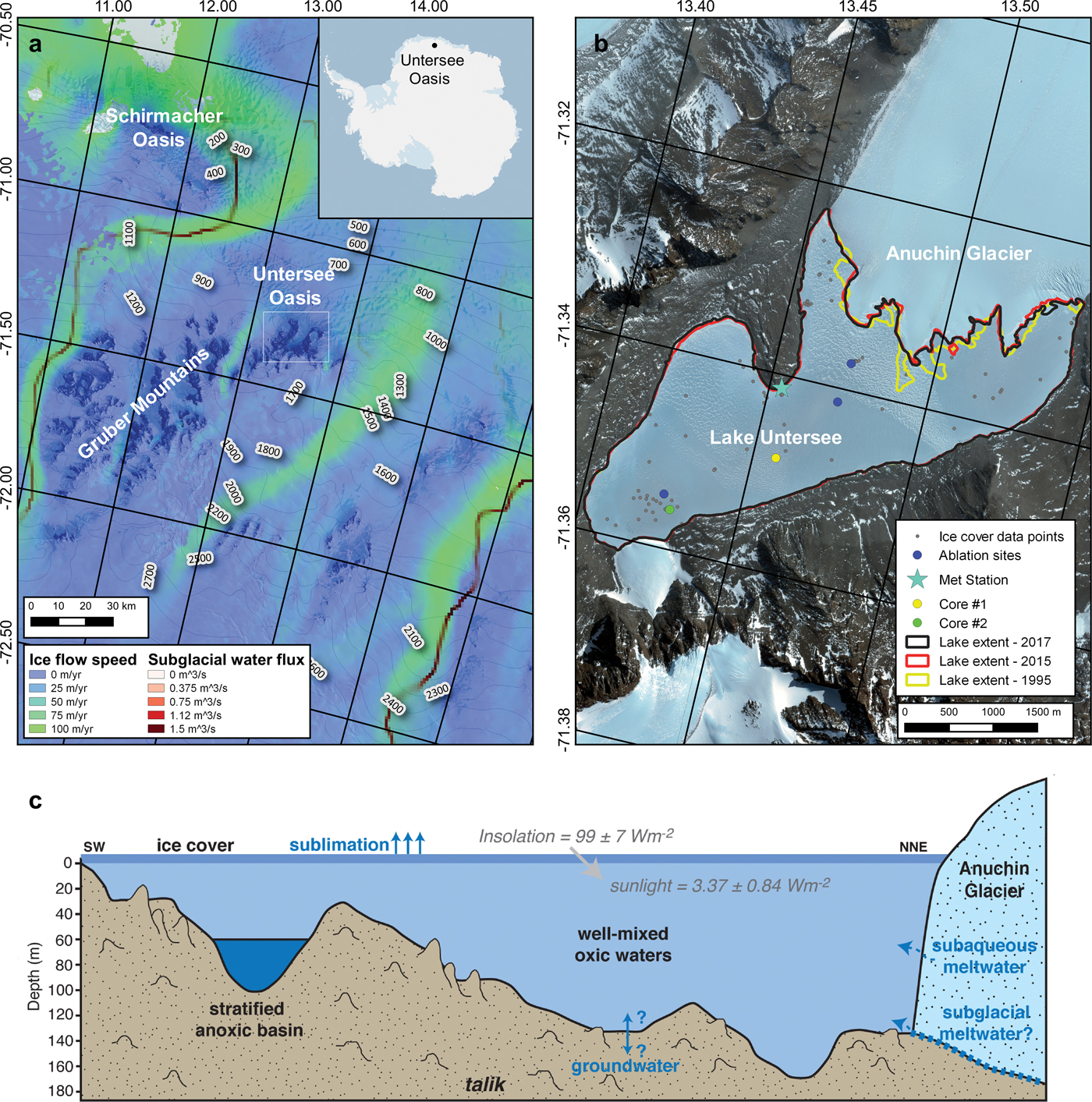
Fig. 1. Maps and cross-section showing: a. the location of the Untersee Oasis, adjacent regional ice-stream velocities (from Rignot et al. Reference Rignot, Mouginot and Scheuchl2017) and regional subglacial water fluxes (from Le Brocq et al. Reference Le Brocq, Ross, Griggs, Bingham, Corr and Ferraccioli2013), b. location of ice-cover data sampling points (i.e. thickness, density), ablation measurement sites and ice cores on Lake Untersee's ice cover, and c. Lake Untersee's bathymetry, ice-cover solar radiation transmissivity and proposed input and output sources.
Lake Untersee is located in a closed basin at c. 610 m a.s.l. and is dammed at its northern end by the Anuchin Glacier where a pressure ridge forms at the lake–glacier interface (Fig. 1). The lake is 2.5 km wide and 6.5 km long, making it the largest freshwater lake in central Queen Maud Land (Hermichen et al. Reference Hermichen, Kowski and Wand1985). With the exception of a boulder field at the south end of the lake and other large boulders scattered across the lake, the surface of ice cover on Lake Untersee is smooth and free of any fine sediments. The lake has two sub-basins: 1) a large basin occupies the northern and central section to a maximum depth of 169 m, and 2) a shallower basin occupies its southern section to depth of 100 m. The two basins are separated by a sill that cuts across the lake at 50 m depth (Wand et al. Reference Wand, Schwarz, Brüggemann and Bräuer1997). The water in the larger and deeper basin and above the sill in the shallower basin is well mixed and has a temperature near 0.5°C, pH near 10.6, dissolved oxygen near 150% and specific conductivity near 505 μS cm−1 (Wand et al. Reference Wand, Schwarz, Brüggemann and Bräuer1997, Reference Wand, Samarkin, Nitzsche and Hubberten2006, Andersen et al. Reference Andersen, Sumner, Hawes, Webster-Brown and McKay2011). The presence of the ice wall at the lake–glacier interface results in buoyancy-driven convection, allowing effective mixing throughout most of the lake with timescales of 1 month (Steel et al. Reference Steel, McKay and Andersen2015). However, in the southern basin, the water below the sill (60–100 m) is stratified, with temperatures ranging between 3°C and 5°C, lower pH (c. 7), higher specific conductivity (1100–1300 μS cm−1) and dissolved oxygen levels near 0%. This anoxic water does not mix with the overlying oxic water due to its higher density (Bevington et al. Reference Bevington, McKay, Davila, Hawes, Tanabe and Andersen2018). The floor of the oxic sub-basin in Lake Untersee is covered by photosynthetic microbial mats, with the transparency of the lake ice to photosynthetically active radiation (PAR) being 4.9 ± 0.9% (Andersen et al. Reference Andersen, Sumner, Hawes, Webster-Brown and McKay2011).
The climate in the Untersee Oasis is part of a polar desert regime. Ten years of climate data (2008–2017) collected by an automated weather station along the shore of Lake Untersee (71.34°S, 13.45°E, 612 m a.s.l.) shows a mean insolation of 99 ± 7 W m−2, mean annual air temperature (MAAT) of -9.5 ± 0.7°C, thawing degree-days ranging from 7 to 51 degree-days and a mean relative humidity of 42 ± 5% (Table I). The MAAT showed little to no change over the past decade (Table I). The average wind speed was 5.4 m s−1, with a strong south wind descending from the polar plateau and sweeping across the southern section of the lake and also a strong east wind descending from the Aurkjosen Cirque and flowing across the snout of the Anuchin Glacier. Despite having a relatively warm MAAT for Antarctica, the climate in the oasis is dominated by intense ablation, which limits surface melt features due to cooling associated with latent heat of sublimation (e.g. Hoffman et al. Reference Hoffman, Fountain and Liston2008).
Table I. Inter-annual summer comparison of climatic data in the Untersee Oasis during the 2008–2018 period.

aStarting after 8 Dec 2008.
bCorrect here (cf. Andersen et al. Reference Andersen, McKay and Lagun2015 incorrect in table 1, correct monthly averages in table 2).
c48.8 degree-days excluding Nov 2012 (cf. Andersen et al. Reference Andersen, McKay and Lagun2015).
dHigh temperatures corrected for loss of solar shield (11 Sep 2013–9 Dec 2014).
eNot available due to winter battery failure.
fData from Data Garrison Station.
Methodologies
Ice thickness and density of ice cover
During each expedition to Lake Untersee since 2008, holes were drilled through the ice cover using a 10 inch Jiffy drill. The ice thickness and freeboard (difference between height of the surface of the ice and water in the borehole) was determined using a 4 m pole graduated at 1 cm. From these two measurements, the density of the ice cover (in kg m−3) was calculated from:
 $$\rho _{ice} = \left( {1-\displaystyle{{Fb_i} \over {H_i}}} \right) \times 1000$$
where Fb i = freeboard (in cm) and H i = thickness of ice cover (in cm).
Given the dimension of the lake, the locations of most drill holes were randomly selected, with one repeat location to verify ice thickness changes over time. The location of each drill hole (n = 84) was recorded with a handheld Garmin GPSMAP 64s GPS with accuracy of ± 3 m and the ice thickness and density data were added as points to ArcMap. The values were interpolated with ordinary spherical kriging where parameters (number of lags: 12 points; sector type: 8 sectors; maximum and minimum neighbours: 5 and 2) were set to obtain the lowest root-mean-square error. The interpolated results were displayed on a common scale and overlaid on a WorldView satellite image (acquisition date: 7 December 2015).
Ice cover ablation rates
Wand et al. (1996) reported the first ablation measurements at Lake Untersee based on measurement of three wooden ablation stakes in the ice cover; each was 4.5 cm in diameter and 4 m long and covered with white reflective tape. They reported ablation of the ice over 12 days in February 1995 was by 1 cm at the north end of the lake, 3 cm at the south end of the lake and 2.5 cm midway. No detailed descriptions of the ablation stakes as observed the following year were published.
On 7 December 2008, we inserted ablation ropes (c. 10 m lengths of braided 5 mm diameter white polyester) into seven holes drilled through the ice on a north–south transect, similar to that used by Wand et al. (1996), as well as five holes in the north-east and north-west corners of the lake (Fig. 1). Holes were backfilled with snow and ice to ensure the lines froze into the 15 cm diameter drill holes. Three years later, we recovered some but not all of the ablation lines; extensive snow cover on the lake that year made the finding and recovery of the ropes difficult.
Ice cover freezing rates
An approach to quantifying the amount of ice freezing at the ice–water interface based on the properties of the ice in the ice cover has not yet been developed for perennially ice-covered lakes. The abundance of gas bubbles occluded in the ice cover should vary as freezing progresses and excess dissolved air develops in the water (Lipp et al. Reference Lipp, Korber, Englich, Hartmann and Rau1987, Killawee et al. Reference Killawee, Fairchild, Tison, Janssens and Lorrain1998). The stable isotopes of water (δD-δ18O) will also evolve during closed-system freezing, such as for the ice cover of Lake Untersee (i.e. Lacelle Reference Lacelle2011). Given that freezing at the ice–water interface largely occurs in winters (i.e. Clow et al. Reference Clow, McKay, Simmons and Wharton1988, Dugan et al. Reference Dugan, Obryk and Doran2013), the bubble abundance and δD-δ18O values in the ice cover should reflect seasonal freezing of the water.
To verify whether the bubble abundance and δD-δ18O values in the ice cover preserve information related to freezing rates, the ice cover of Lake Untersee was sampled at its central and southern sectors in December 2017 (Fig. 1). The ice was sampled using a Cold Regions Research and Engineering Laboratory (CRREL) coring kit to a depth of c. 2 m to prevent mixing with lake water. The ice cores were first photographed in the field under a light table using a Nikon D850 camera (focal length of 35 mm and exposure time of 1/20 s). The ice cores were then sliced at 2 cm, allowed to melt in sealed Ziploc bags, transferred in high-density polyethylene bottles and shipped in coolers to the University of Ottawa, where they were stored at 4°C until analysis.
The distribution and morphology of air bubbles in the ice cover were extracted from the photographs of the ice cores using the ImageJ software. The photographs were first converted to 8-bit grayscale format and classified following thresholding as either: 1) area occupied by bubbles; or 2) bubble-free area. The size and distribution of the bubbles were extracted at 1 cm slices using the analyze particles tool (e.g. Kinnard et al. Reference Kinnard, Koerner, Zdanowicz, Fisher, Zheng and Sharp2008).
The 18O/16O and D/H ratios were determined using a Los Gatos Research liquid water analyser coupled to a CTC liquid chromatography prep-and-load autosampler for simultaneous 18O/16O and D/H ratio measurements of H2O and verified for spectral interference contamination. The results are presented using the δ-notation (δ18O and δD), where δ represents the parts per thousand differences for 18O/16O or D/H in a sample with respect to Vienna Standard Mean Ocean Water (VSMOW). Analytical reproducibility values for δ18O and δD were ± 0.3‰ and ± 1‰, respectively. Deuterium excess (d) was then calculated using the following equation: d = δD – 8δ18O (Dansgaard Reference Dansgaard1964).
The periodicity of bubble content (%) and the distribution of δ18O values were extracted via spectral analysis (Fourier transformation) using R software's Spectrum tool (Stats built-in package). Significant-amplitude spectrum peaks indicate the periodicity of freezing events. The frequencies were converted to annual ice accretion using the following equation:
 $$\hbox{Annual ice accretion} = \displaystyle{1 \over x} \times SI$$
where x = peak frequency and SI = sampling interval (here 2 cm) (Blackman & Tuckey Reference Blackman and Tukey1958).
Water mass balance of Lake Untersee
Lake Untersee is a closed-basin lake dammed at its northern end by the Anuchin Glacier. As such, the water mass balance of the lake can be determined from:
 $${\rm \Delta} S = P + I_s + I_e + I_g-O_s-O_g$$
where ΔS = change in the volume of water, P is total annual precipitation, I s, I e and I g are the inflows of surface water, subaqueous melting of terminus ice (originating from the melting of the submerged Anuchin Glacier at the ice–lake water interface) and groundwater (subglacial meltwater or other sources), respectively, and O s and O g are the outflows of surface water and groundwater, respectively.
The volume of water in Lake Untersee was determined from the bathymetry map of Wand et al. (Reference Wand, Samarkin, Nitzsche and Hubberten2006), which was digitized and georeferenced in the ArcMap software. The relations between lake surface elevation, surface area and water volume were also compiled from the digitized bathymetry map. Changes in lake surface area between 1995 and 2017 were then determined using the Geomaud 1995 air photographs, which were digitized and georeferenced in ArcMap, and with the use of 2015 and 2017 WorldView satellite images (acquisition dates: 7 December 2015, 7 December 2017; image resolution: 50 cm). The lake extents in 1995, 2015 and 2017 were traced in ArcMap (World Geodetic System 1984; Universal Transverse Mercator Zone 33S) and the surface area computed from the derived polygons.
The sealed nature of Lake Untersee is such that direct precipitation (P) is likely not contributing to its water mass balance. The contribution of subaqueous melting of terminus ice from the Anuchin Glacier (I e) was determined from its average annual velocity, its cross-sectional area at the ice–water interface (which assumes the glacier is grounded at the lake bed) and changes in the position of the glacial ice tongues at the contact with the lake. The velocity of the Anuchin Glacier was obtained by tracking the displacement of a target on its surface over a 10 year period (2008–2017). The position of the target was recorded with a handheld Garmin GPSMAP 64s GPS with accuracy of ± 3 m. The target velocity data were compared to the 2011–2017 NASA MEaSUREs Antarctic ice velocity (Rignot et al. Reference Rignot, Mouginot and Scheuchl2017). The outflow of surface water (O s) was determined from our calculation of the amount of ice loss by ablation.
Results
Thickness and density of the ice cover
Ice thickness measurements taken at the same location between 2011 and 2017 provided near-identical results (3.78 ± 0.07 m; n = 4), indicating that measurements obtained over a 10 year period should have little effect on estimating ice thickness. The measurements of the ice cover thickness range from 1.96 to 3.96 m, with a bimodal distribution (median = 2.52 m; average = 2.76 ± 0.59 m; n = 89). Based on geostatistical kriging interpolation, the average lake ice thickness is 2.77 ± 0.25 m. Ice thickness shows a general north–south trend, with thicker ice cover in the north-west sector and thinner ice in the south and north-east sectors (Fig. 2). The density of the ice cover ranges from 764 to 1000 kg m−3, with an average of 902 ± 47 kg m−3. Geostatistical interpolation indicates an average ice density of 891 ± 5 kg m−3. Under-dense ice (< 850 kg m−3) is found in the central section of the lake, due east of the moraine, and over-dense ice (near 1000 kg m−3) is found in the north-east sector.
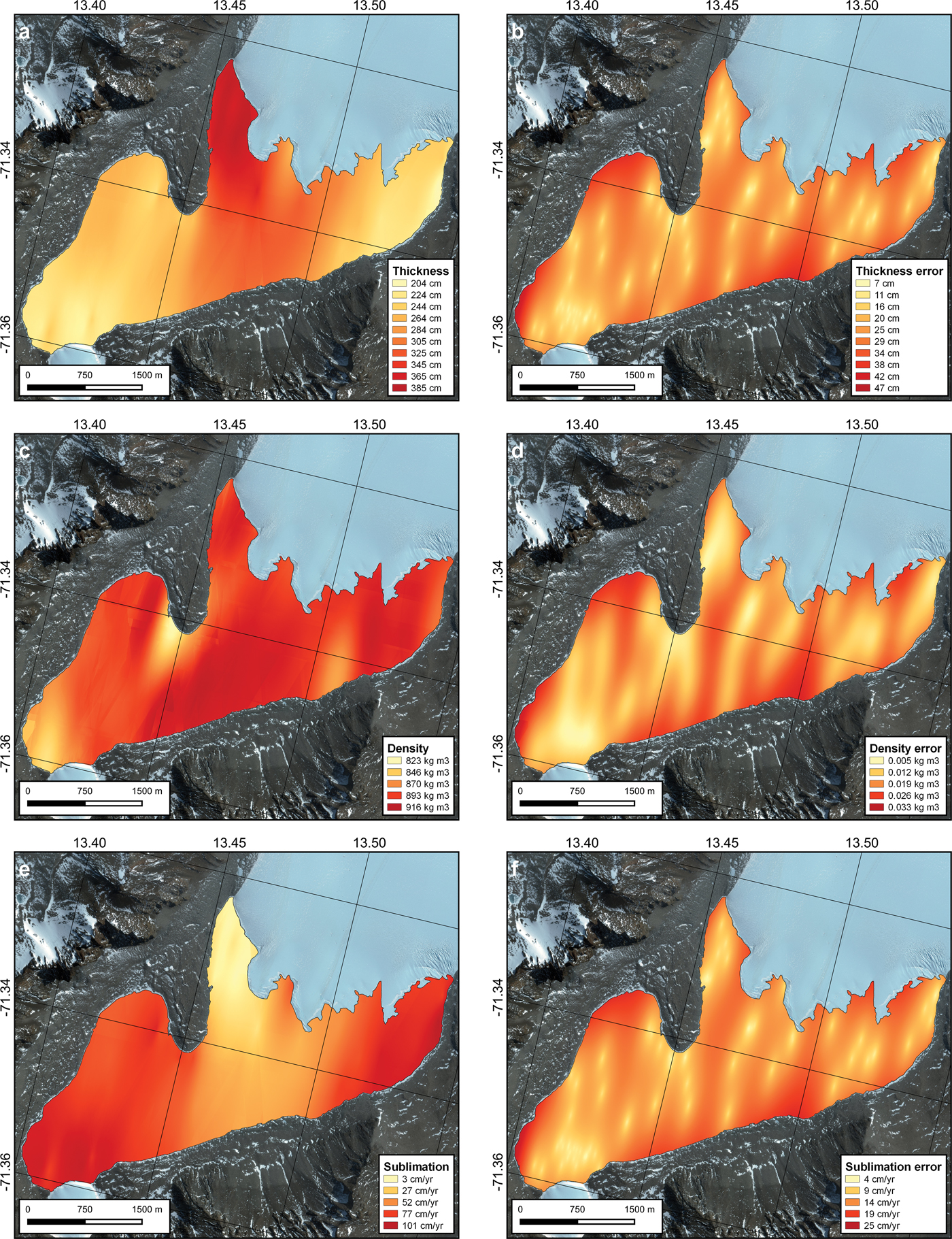
Fig. 2. WorldView images (7 December 2017) of Lake Untersee showing: a. interpolated ice-cover thickness, b. interpolated ice-cover thickness errors, c. interpolated ice-cover density, d. interpolated ice-cover density errors, e. interpolated annual ice-cover sublimation rate, and f. interpolated annual ice-cover sublimation rate errors.
Ablation rates from ablation ropes
On 17 November 2011, two ablation ropes at the southern end of the lake indicated net ablations of 230 and 213 cm over 3 years. On 18 December 2011, an additional 7 cm of ablation was measured. These results indicate annual average ablation rates of 78 and 72 cm yr−1 at the two sites. Three ablation ropes due east of the meteorological station (central area of the lake) indicated ablations of 116, 117 and 122 cm, corresponding to annual average ablation rates of 39, 41 and 39 cm yr−1, respectively. From this, we infer that the yearly ablation rate is c. 40 ± 1.2 cm yr−1 in the central portion of the lake, and it increases to c. 75 ± 4.2 cm yr−1 at the southern end of the lake, where some of the thinnest ice is also observed.
Freezing rates from bubble morphology and δD-δ18O composition of ice cover
The ice cover of Lake Untersee contains a range of bubble sizes and shapes (Fig. 3). In both ice cores, the shapes of the bubbles were either spherical, oval, dendritic or tubular. The ice cover in the central sector had a bubble content ranging from 2% to 50%, with higher bubble content and variability in the uppermost 75 cm (peak of 50% at 54 cm depth) (Fig. 4). Bubble content was more constant below 100 cm, where it varied between 2% and 18%. The ice cover in the southern sector had bubble contents ranging from 0.3% to 46%, with higher bubble contents in the uppermost 150 cm. No particular trend was observed for the bubble content, but three peaks were identified at depths of 18, 85 and 135 cm. The δ18O values in the ice core from the central sector ranged from -35.5‰ to -34.2‰, whereas D-excess values ranged from -1.31‰ to 6.9‰. The δ18O and D-excess values showed decreasing and increasing trends with depth, respectively. The δ18O values in the southern sector ice fluctuated from -36.2‰ to -35.6‰, with D-excess varying from -8.8‰ to 11.4‰. Variations in δ18O and D-excess values were negatively correlated in the uppermost 50 cm; this was reflected to a lesser degree in the lower portion of the core, where δ18O and D-excess values were much more stable.
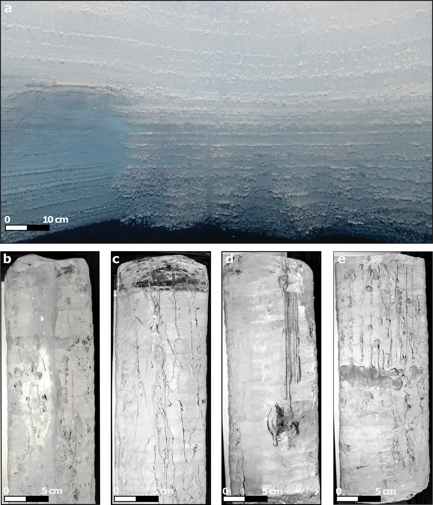
Fig. 3. Ice-cover bubble abundance and morphology. a. Underwater view of bubbles in the lower portion of the ice cover; b.–e. examples of different morphologies of bubbles observed in ice cover: b. spherical bubbles in core #1, c. dendritic bubbles in core #1, d. tubular and oval bubbles in core #2, and e. tubular and spherical bubbles in core #2.

Fig. 4. Depth profiles of bubble content (%), δ18O and D-excess measurements in a.–c. core #1, and d.–f. core #2. Modelled annual ice-cover coevolution of δ18O ratios and D-excess is shown in grey.
The spectral power for the distribution of bubble abundance and δ18O showed peaks at 0.041 and 0.022 for the core retrieved from the central and southern sectors of the lake, respectively (Fig. 5). The frequencies were converted to annual ice accretion ((1 / frequency) × 2 cm) and provided freezing rates of 49 cm yr−1 at the central section and 91 cm yr−1 at the southern section of the lake.

Fig. 5. Amplitude spectra in radians for δ18O and bubble content (%) in (a. & c.) core #1, and (b. & d.) core #2. Frequencies can be converted to annual ice accretion (1/X × 2), where X is the peak frequency. The dotted lines indicate the peak of the spectral signal frequencies for core #1 (c. 0.041 = 49 cm) and for core #2 (c. 0.022 = 91 cm). Amplitude spectra for modelled seasonal ice-cover freezing rates (using a simple Rayleigh-type fractionation of the residual water) of 49 cm (core #1) and 91 cm (core #2) are shown in e. and f., respectively.
Water mass balance of Lake Untersee
Analysis of the bathymetry of Lake Untersee with the Surface Volume tool in 3D Analyst (ArcGIS 10 software) demonstrates that lake surface area and lake water level are positively correlated; it is only when the lake level is below 520 m that a further lowering of the water level results in small changes in surface area (Fig. 6). Based on the digitized bathymetry, Lake Untersee has a water volume of 5.21 × 10⁸ m−3. In 2017 and 2015, Lake Untersee had surface areas of 8.73 and 8.72 km2, respectively, values that are slightly greater than what was measured in 1995 (8.45 km2). The difference in surface area between 1995 and 2017 is caused by two of the Anuchin Glacier's ice tongues that retreated by 420 and 480 m, respectively. Visual comparison of oblique air photographs from 1939 also show little variation in the extent of Lake Untersee, which implies that its extent has been relatively stable for the past 80 years. The ice cover where the ice tongues had receded is composed of both lake ice and patches of white glacier ice that have been smoothly ablated to the same elevation as the lake ice (Fig. 1b). Unlike the lake ice that is sediment free, the patches of glacier ice in the ice cover contain cryoconite holes.
Fig. 6. Relation between lake surface elevation and a. surface area, and b. water volume. c. Relation between surface area and water volume. The dashed line is the best fit polynomial line. Analysis derived from bathymetry from Wand et al. (Reference Wand, Samarkin, Nitzsche and Hubberten2006).
The amount of direct precipitation (P) and inflow of surface water (I s) contributing to the water mass balance of Lake Untersee can be ignored because: 1) the lake does not develop a moat in summer and hence rainfall cannot directly contribute to lake water; 2) no ephemeral streams feeding into the lake were historically observed; and 3) any snow that falls on the ice cover quickly sublimates or is blown away. The volume of subaqueous melting of terminus ice (I e) was estimated from the velocity of the Anuchin Glacier, its cross-sectional area along the ice–water interface and changes in the location of the glacial ice tongues. A target placed on the surface of the Anuchin Glacier moved 76 m at an azimuth of 183° between 2008 and 2017, which corresponds to a mean annual ice velocity of 8.4 m yr−1, which is in the range reported by MEaSUREs annual Antarctic ice velocity (c. 8–9 m yr−1 on average between 2011 and 2017; Fig. 1). Based on the bathymetry along the lake–glacier interface and the width of the glacier along the lake, the cross-sectional area of the ice wall is estimated to be 0.27 km2. Therefore, subaqueous melting of the Anuchin Glacier's terminus contributes annually 1.98–2.23 × 10⁶ m3 of water volume to the lake. The volume of surface water (O s) loss was determined from our calculation of ablation of the ice cover, which ranges between c. 40 cm yr−1 in the central portion of the lake and increases to c. 75–80 cm yr−1 in the southern end of the lake. The range in rates of annual ablation translates into annual water loss in the order of 3.22–6.43 × 10⁶ m3 (0.6–1.2% of the lake's volume).
Discussion
Spatial variations in ice cover thickness and ablation/freezing rates
The ice cover of Lake Untersee is in steady state because its thickness at the same location did not change between 2011 and 2017 (3.78 ± 0.07 m; n = 4). This means that the freezing and ablation rates of the ice cover must be near equal (e.g. McKay et al. Reference McKay, Clow, Wharton and Squyres1985). Our measurements from in situ ablation ropes provided ablation rates of c. 40 ± 1.2 cm yr−1 and c. 75 ± 4.2 cm yr−1 in the northern and southern sectors, respectively. The freezing rates derived from the frequency distribution of the bubbles and δ18O vertical profiles in the ice cover yielded values of 49 ± 2 cm yr−1 in the central sector and 91 ± 2 cm yr−1 at the southern sector of the lake, similar to the nearby ablation rates.
Lipp et al. (Reference Lipp, Korber, Englich, Hartmann and Rau1987) observed, although at a smaller scale, dendritic breakdown of the planar ice–water interface due to gas enrichment and bubbles nucleated in interdentritic spaces under closed-system freezing experiments of highly saturated gas solutions. Nucleation and growth of gas bubbles were seen to be periodic processes under certain circumstances, which was explained by the continuous build-up and reduction of the concentration of gases in the remaining solution. The δD-δ18O measurements also allow for the determination of freezing events because in closed-system equilibrium freezing a progressive depletion in 18O and D values in the residual water (and forming ice) occurs following Rayleigh-type fractionation (Lacelle 2001). In perennially ice-covered lakes, where repeated freezing occurs at the bottom of the ice cover, an isotopic discontinuity should separate the seasonal freezing events in the ice cover when the water column is well mixed, and this should be reflected in the δ18O profile. The δ18O composition of the ice cover during seasonal freezing was modelled using a simple Rayleigh-type fractionation of the residual water to assess whether the profile and the extracted frequency are similar to our measurements. The model assumes equilibrium freezing of 1% of the lake water (reflecting the amount of water that sublimates and that must freeze to maintain water balance) in 0.01% residual water fraction steps using the fractionation factors corrected for initial δD-δ18O water composition (i.e. Jouzel & Souchez Reference Jouzel and Souchez1982) with an introduced noise signal of 100% variance and repeated for three to five freezing cycles. The modelled freezing thickness was adjusted to both coring sites (i.e. 49 and 91 cm yr−1). The δ18O composition of the ice cover matched well with the measured profile and spectral frequencies in both cores (Figs 4 & 5). The D-excess values obtained from this modelling also gave a good fit with the profile measurements. It thus appears that the frequency distribution of δ18O and the bubble content in the ice cover preserves information about the thickness of annual freezing at the bottom of the ice cover.
The thickness of the ice cover of the 6.5 km long Lake Untersee shows a general north–south trend, with thicker ice cover in the north-west sector (c. 3.50–3.96 ± 0.10 m) and thinner ice in the south and north-east sectors (c. 1.96–2.50 ± 0.10 m). The ice cover is thinner than most of the ice-covered lakes in the MDV, where they range from 3 to 6 m, despite considerable variations in depth, temperature and salinity between the lakes (Doran et al. Reference Doran, McKay, Clow, Dana, Fountain and Nylen2002). A significant negative relation exists between the ice thickness and ablation/freezing rates (Fig. 7). The relation was used to derive the ablation rate across the entire lake using geostatistical interpolation, which averaged 61 ± 13 cm yr−1 (median = 68 cm yr−1). Like the systematic increase in ice thickness from north to south in the lake, the ablation rates increase along this same direction; this suggest that ablation has a strong controlling effect on ice thickness. Considering the little change over the past decade in insolation, MAAT, thawing degree-days and relative humidity (Table I), the spatial variation in ablation rates across the ice cover is likely due to the persistent strong south winds descending from the Sjobotnen Cirque and sweeping across the southern section of the lake (average wind speed of 4.9 m s−1 in summer 2011) and also the strong east wind descending from the Aurkjosen Cirque (average wind speed of 6.2 m s−1 in summer 2011) and flowing across the snout of the Anuchin Glacier. The central area of the lake where the thicker ice is found is sheltered from the strong winds (average wind speed of 4.2 m s−1 in summer 2011), as evidence of the snow-shadow on the lake ice (Fig. 1b).
Fig. 7. Relation between the ice-cover thickness and ablation/freezing rates. White and black squares indicate freezing rates inferred from spectral analysis of ice-cover cores and measured ice-cover sublimation rates, respectively.
Heat energy model of the ice cover
Clow et al. (Reference Clow, McKay, Simmons and Wharton1988) developed a climate-based model that incorporated non-steady molecular diffusion into Kolmogorov-scale eddies to derive the average sublimation rate of the ice cover of lakes in the MDV (c. 30 cm yr−1). Given that the MAAT at Lake Untersee is c. 7°C warmer than that used by Clow et al. (Reference Clow, McKay, Simmons and Wharton1988), the sublimation rate of the ice cover of Lake Untersee is expected to be c. 1.8× higher, a factor given by the ratio of the vapour pressure of ice at -9.5°C and -17.0°C. This first-order scaling would predict an average sublimation rate at Lake Untersee of 60 cm yr−1, similar to the average ablation rate of 61 ± 13 cm yr−1. However, the thickness of the ice cover of Lake Untersee has a strong spatial variation that appears to be associated with the wind regime across the lake. To test for the effect of wind on sublimation rates, we assume that the energy required to sublimate the ice comes from turbulent heat flux caused by the wind blowing over the ice surface (i.e. Paterson Reference Paterson2010). We used a standard turbulent heat flux equation for smooth-surface ice to calculate the thickness of ice that can sublimate annually from variable wind speeds (SR, in m yr−1) using:
 $$SR = \displaystyle{{22.2\; A\; u\; \lpar {e_s-e} \rpar t{\rm \;}} \over {L_v\rho _{ice}}}$$
where A = 0.002 (the transfer coefficient for air moving over smooth ice with temperatures in the -10°C to 0°C range; Ambach & Kirchlechner Reference Ambach and Kirchlechner1986), u is the wind speed (m s−1) at screen height (1 m), e s is the saturation water vapour pressure over ice (at the ice surface temperature in Pa; a value that is c. 600 Pa for ice near 0°C) and e is the water vapour pressure at screen height (relative humidity = 42%, so e ≈ 252 Pa), t is the number of seconds in a year (3.153 × 10⁷), L v is latent heat of vaporization (3.1335 × 10⁶ J kg−1) and ρ ice is the density of ice (917 kg m−3).
The theoretical amount of sublimating ice as a result of turbulent heat flux shows a linear relation with wind speed blowing over the ice surface (Fig. 8). Our measured summer 2011 average wind speeds and sublimation rates show good fit with the theoretical line. The locations on the lake with slightly lower sublimation rates than predicted is attributed to the presence of snow on the ice surface, which would decrease the time during which sublimation is occurring (i.e. it would reduce the value of t in Eq. (4) to < 1 year). Therefore, variations in sublimation rates on the ice cover appears to be largely influenced by wind and associated with its turbulent heat flux and the number of snow-covered days (which reduce the sublimation of the ice cover).
Fig. 8. Relation between wind speeds and sublimation rates at three locations on the ice cover. See Fig. 1 for the locations of the sites.
Water mass balance and heat energy model of Lake Untersee
Lake Untersee has a water volume of 5.21 × 10⁸ m−3 and has remained stable since at least 1995 and was most likely stable for the past 80 years. With a surface area of 8.73 km2 and an average sublimation rate of 61 ± 13 cm yr−1, Lake Untersee is losing annually 4.90 ± 1.03 × 10⁶ m3 of water (0.94 ± 0.20% of total lake water volume). Assuming that sublimation from the ice cover is the only output of water for the lake, then the lake must receive an equal inflow to maintain the water budget in equilibrium. There are no visible inflows of surface water to the lake, and direct precipitation does not contribute to the lake water. Hermichen et al. (Reference Hermichen, Kowski and Wand1985) inferred that the lake was being recharged by melting of the Anuchin Glacier with no distinction between subaqueous melting of terminus ice and subglacial meltwater or other potential groundwater sources. The Anuchin Glacier advances towards Lake Untersee at a velocity of 8–9 m yr−1, and since the ice tongues at the glacier–lake interface have remained at the same location for at least the past 30 years, subaqueous melting of terminus ice contributes 1.98–2.42 × 10⁶ m3 to the lake annually (40–45% of annual lake water volume; Fig. 9a). Therefore, c. 2.68–2.92 × 10⁶ m3 (55–60% of annual lake water volume) must be contributed annually from subglacial meltwater and/or a distinct groundwater source. This equates to a discharge of c. 8.8 × 10⁻² m3 s−1, a reasonable flux given the reported range of subglacial water flux in the region (Fig. 1a). Therefore, Lake Untersee must be hydrologically connected to a regional groundwater system, similar to what has been inferred for Lake Bonney in the MDV from airborne transient electromagnetic sensors (i.e. Mikucki et al. Reference Mikucki, Auken, Tulaczyk, Virginia, Schamper and Sørensen2015).

Fig. 9. a. Annual contribution of subaqueous melting of terminus ice to Lake Untersee as a function of various ice-cover sublimation rates and glacial velocities. b. Transmissivity of the ice cover to visible light (based on photosynthetically active radiation measurements) as a function of ice thickness. SE = standard error.
Unlike the lakes in the MDV, there are no visible surface inflows of water to the lake that would bring sensible heat energy to the lake water. Therefore, the subaqueous melting of terminus ice must be accomplished by sunlight energy that penetrates the ice cover. To test whether there is enough sunlight that reaches the water column to melt annually 1.98–2.23 × 10⁶ m3 of the terminus of the Anuchin Glacier, we undertook an energy mass balance calculation. Previous studies (e.g. McKay et al. Reference McKay, Clow, Wharton and Squyres1985, Palmisano & Simmons Reference Palmisano and Simmons1987) have used a simple Beer's Law, exp(-z/H), to estimate ice cover light penetration and fitted scale height (H) to PAR measurements (where z is the ice cover thickness). This is incorrect in two ways: 1) in ice cover, scattering dominates over absorption and Beer's Law is for absorption only, and 2) the properties of the ice are not uniform over the PAR measurements. Here we use a simple scattering model for the lake ice cover that: 1) assumes uniform optical properties with depth, consistent with observations (absorption by very clean ice and scattering by large bubbles) (Fig. 3); 2) uses the absorption coefficient in ice as a function of wavelength from the latest compilation (i.e. Warren & Brandt Reference Warren and Brandt2008); and 3) uses a two-stream scattering model that includes absorption (i.e. eqs (3)–(7) in Sagan & Pollack Reference Sagan and Pollack1967). There are two key parameters to this model: the total scattering optical depth and the scattering asymmetry factor. Given that ice is transparent mainly to the visible portion of the spectrum, a wavelength-resolved analysis was performed from 350 to 850 nm, which treated 850–3200 nm as a completely absorbing black body. Using our two measurements beneath the ice cover (PAR albedo = 0.66 and transmittivity = 0.049; Andersen et al. Reference Andersen, Sumner, Hawes, Webster-Brown and McKay2011) and assuming isotropic scattering by the bubbles in the ice cover to derive a fit to PAR measurements, we obtain a scattering optical depth of 9 m. The comparison to PAR measurements is determined by the average of 400–700 nm, weighted by the relative photon flux at each wavelength.
The flux of sunlight that penetrates the ice cover is determined by summing the computed solar flux transmissivity from 350 to 850 nm and the measured surface radiation (99 ± 0.7 W m−2) from Andersen et al. (Reference Andersen, McKay and Lagun2015). Averaging over the range of the thickness of the ice cover (1.96–3.96 m), the energy reaching the water column is 3.37 ± 0.84 W m−2; an amount that is sensitive to ice thickness (Fig. 9b). Neglecting loses of energy to the sides or bottom of the lake, which are expected to be minor, the mass of ice melted at the glacier–lake water interface is directly related to the solar energy entering the water column and can be calculated from:
 $$Ice\_melt = \lpar {SoAt/L} \rpar {\rm} / \rho _{ice}$$
where Ice_melt is the annual volume of ice melted (m3 yr−1), So is the solar flux entering the water column (W m−2), A is the area of the lake (m2), t is time in seconds, L is the latent heat of fusion of ice (J kg−1) and ρ ice is the density of ice.
According to Eq. (5), the 3.37 ± 0.84 W m−2 solar flux that enters the water column can melt 2.79 × 10⁶ m3 yr−1, which is enough to sustain the annual contribution of the subaqueous melting of terminus ice (1.98–2.23 × 10⁶ m3). Considering that the annual contribution of subaqueous melting of terminus ice is dependent on the velocity of the Anuchin Glacier, there would be enough sunlight energy entering the water column to sustain subaqueous melting for contributions of up to 54%, an equivalent in glacier velocity of up to 11.4 m yr−1.
Lake Untersee and changing climate
Lakes are good indicators of climate change because of their physical, chemical and biological responsivity to changes in environmental conditions (Williamson et al. Reference Williamson, Saros, Vincent and Smol2009). Ten year measurements of ice-cover thickness of Lake Untersee showed little change; this is in contrast to lakes in the MDV that decreased by over 2 m between 1999 and 2016 (Obryk et al. Reference Obryk, Doran and Priscu2019). The Untersee Oasis has a relatively warm MAAT for Antarctica; in fact, it is c. 7°C warmer than in the coastal zone in the MDV (i.e. Clow et al. Reference Clow, McKay, Simmons and Wharton1988, Doran et al. Reference Doran, McKay, Clow, Dana, Fountain and Nylen2002). Our climate measurements indicate that the MAAT in the Untersee Oasis has been relatively stable during the past decade (2008–2018; Table I). This is in contrast to the rest of the Queen Maud Land region, where MAAT has increased at a rate of 1.1 ± 0.7°C per decade between 1998 and 2016 (Medley et al. Reference Medley, McConnell, Neumann, Reijmer, Chellman and Sigl2018), and with the MDV, where air temperature has increased since 2006 with no distinct trend (Obryk et al. Reference Obryk, Doran and Priscu2019). Compared to the MDV ice-covered lakes, Lake Untersee should be developing a moat in summer, given the similar range in thawing degree-days (7–51) and higher MAAT; however, no moat develops around Lake Untersee, even during summers with a high number of thawing degree-days. A minor increase in summer air temperature is not expected to alter this condition, as the region is dominated by intense sublimation, which limits surface melt features and prevents summer moats from developing around the edges of the lake due to the cooling associated with the latent heat of sublimation (e.g. Hoffman et al. Reference Hoffman, Fountain and Liston2008). However, a change in wind regime should have a significant impact on the lake ice dynamic as it largely drives the sublimation and controls the thickness of the ice cover and consequently the proportion of solar radiation that enters the water column.
A more direct impact of climate change on the hydrology of Lake Untersee would be its effect on the surrounding glaciers, namely the Anuchin Glacier. Currently, the Anuchin Glacier has a velocity of 8–9 m yr−1, and given that the position of the glacier–lake interface has not changed over the past 10 years, we assume that the amount by which the glacier advances all melts and contributes c. 40–45% of the annual lake water volume input. However, under the current ice cover thickness configuration, only c. 3.37 W m−2 of sunlight reaches the water column, which provides enough energy to melt a maximum of 2.79 × 10⁻³ km3 of subaqueous ice along the ice wall. This volume would be exceeded if the velocity of the Anuchin Glacier exceeded 11.4 m yr−1; in that case, lake water level would rise since the glacier would advance and act like a piston and force the water level to increase. On the other hand, a receding Anuchin Glacier would lower the water level by c. 9% of the receding distance (difference in density between ice and water, and the thickness of the glacier is approximately equal to the average depth of the lake). The responses of other potential water sources with regards to climate change are also uncertain. Currently, no surface streams are feeding into Lake Untersee; however, it is possible that, under a warming scenario, the lake would receive a contribution a surface runoff from ephemeral streams and supraglacial runoff. In that case, the lake would receive sensible and latent heat, which would drastically alter the hydrochemical conditions (i.e. allowing for interactions with the atmosphere) of the lake waters and may cause severe shifts in benthic biochemical regimes. If this happens, Lake Untersee would become more similar to lakes in the coastal MDV.
Conclusions
This study investigated the thermodynamics and the hydrological balance of Lake Untersee, one of the largest perennially ice-covered lakes in East Antarctica. Based on the results, the following conclusions can be drawn:
1. δ18O and bubble content (%) trends in the ice cover can identify the annual thickness of ice accretion, and as such, when combined with ablation rate measurements, steady-state conditions of perennially ice-covered lakes can properly be determined.
2. Ten year measurements at the same location showed that the ice cover had near-identical thickness, indicating that the ice cover is in steady state.
3. The sublimation rate of Lake Untersee (and its control over ice-cover thickness) is largely influenced by wind (its associated turbulent heat flux) and the number of snow-covered days. With an annual average ablation rate of 61 ± 13 cm yr−1, the ice cover has a turnover rate of 3–6 years.
4. Lake Untersee has a water volume of 5.21 × 10⁸ m−3 and is losing annually 0.94 ± 0.20% of total lake water volume. The Anuchin Glacier advances towards Lake Untersee at a velocity of 8–9 m yr−1, and subaqueous melting of terminus ice contributes 40–45% of annual lake water volume; the remaining volume must be contributed annually from subglacial meltwater and/or a groundwater source likely flowing at a rate of c. 8.8 × 10⁻² m3 s−1 into Lake Untersee. This provides one of the first - albeit indirect - pieces of evidence of groundwater recharging lakes in an ice-free region of Antarctica.
5. Based on a simple scattering model for the lake ice cover, 3.37 ± 0.84 W m−2 enters the water column. This provides enough energy to melt the ice along the glacier–lake interface and would be sufficient to sustain melting up to a glacier velocity of 11.4 m yr−1.
Acknowledgements
This work was supported by the TAWANI Foundation of Chicago, the Trottier Family Foundation, the Natural Sciences and Engineering Research Council of Canada (NSERC) Discovery Grant, Polar Knowledge Canada, NASA's Astrobiology Program and the Arctic and Antarctic Research Institute/Russian Antarctic Expedition. A NSERC Alexander Graham Bell Canada Graduate Scholarship (doctoral) provided financial support to B. Faucher. Logistical support was provided by the Antarctic Logistics Centre International (ALCI), Cape Town, South Africa. We are grateful to Colonel (IL) J.N. Pritzker, IL ARNG (retired), of the TAWANI Foundation, Lorne Trottier of the Trottier Family Foundation and fellow field team members for their support during the expedition. We thank the two reviewers for their constructive comments.
Author contributions
Benoit Faucher: paper writing (main contributor); data collection; data analysis and interpretation; editing prior to paper's submission.
Denis Lacelle: paper writing; data collection; data analysis and interpretation; editing prior to paper's submission.
David A. Fisher: data analysis and interpretation; editing prior to paper's submission.
Dale T. Andersen: data collection; data analysis and interpretation; editing prior to paper's submission.
Christopher P. McKay: data collection; data analysis and interpretation; editing prior to paper's submission.
Supplemental data
Datasets are available in the supplementary online material (SOM); SOM 1: 2008–2017 target displacement on Anuchin Glacier; SOM 2: 2008–2018 ice thickness and freeboard measurements of ice cover.
A supplemental file will be found at https://doi.org/10.1017/S0954102019000270.