Introduction
Large earthquake tsunamis, such as the 2004 Sumatra tsunami, can propagate substantial and damaging wave energy to distant coasts through a combination of source focusing and topographic waveguides (Titov et al. Reference Titov, Rabinovich, Mofjeld, Thomson and González2005, Candella et al. Reference Candella, Rabinovich and Thomson2008). Teletsunamis (tsunamis which originated > 1000 km away) could even trigger the Antarctic ice-shelf calving (Brunt et al. Reference Brunt, Okal and MacAyeal2011). The earthquake that occurred off the west coast of northern Sumatra, Indonesia, on 26 December 2004 had an M w above 9.0. The teletsunami was detected in coastal waters with tide gauges at the Chinese Zhongshan Station and Australian Mawson and Casey stations in East Antarctica, around 12 hours after the earthquake. Maximum wave heights of 400–600 mm were recorded (Brolsma Reference Brolsma2005, Zhang et al. Reference Zhang, Huang and Wang2008). The effects of the 2004 tsunami were also recorded at the Japanese Soywa Station, but wave height was much lower (Titov et al. Reference Titov, Rabinovich, Mofjeld, Thomson and González2005).
To date, the effects of tsunamis have been recorded mainly by the DART (Deep-ocean Assessment and Reporting of Tsunami) real-time mooring system (Bernard et al. Reference Bernard, González, Meining and Mulburn2001, Rabinovich et al. Reference Rabinovich, Stroker, Thomson and Davis2011) and by tide gauges in coastal waters (Titov et al. Reference Titov, Rabinovich, Mofjeld, Thomson and González2005, Merrifield et al. Reference Merrifield, Firing and Aarup2005, Rabinovich et al. Reference Rabinovich, Thomson and Stephenson2006). The tide gauge is the main way to perform tsunami detection in Antarctic coastal waters (Titov et al. Reference Titov, Rabinovich, Mofjeld, Thomson and González2005, Brolsma Reference Brolsma2005, Zhang et al. Reference Zhang, Huang and Wang2008). Tsunamis have also been detected by seismometers on ice shelves (floating ice) where the seismometer primarily measures low frequency swell associated with the dispersed tsunami arrival (Okal & MacAyeal Reference Okal and MacAyeal2006). In December 2009, an online coastal mooring system for marine environmental monitoring was deployed in the Great Wall bay near the Chinese Great Wall Station (62°13′S, 58°58′W) off King George Island in West Antarctica. In this paper, we use observation data to analyse the effects of the teletsunamis associated with the great earthquakes near Chile (8.8 M w, 6h34 UT, 27 February 2010) and Japan (9.0 M w, 5h46 UT, 11 March 2011), on Antarctic coastal waters, especially on the sea level oscillations. In addition, water temperature, salinity, pH, and oxidation-reduction potential (ORP), as well as air temperature and wind speed at the time the 2011 Japan tsunami arrived, were analysed in order to understand the consequence of the tsunami on the Antarctic coastal water properties.
Observation and data treatment
Figure 1 shows the locations of the detection site. An online coastal mooring system was deployed in the deepest area in the Great Wall bay, King George Island in 2009. The bay is semi-open with a maximum depth of c. 35 m near the top of the bay. The deploying site is c. 200 m from the coast and c. 30 m underwater. The floats were placed c. 5 m beneath the surface to avoid damage from floating blocks of ice. Electricity is supplied from the Great Wall Station and environmental parameters such as temperature, salinity, depth, pH, PAR (photosynthetically active radiation), ORP, chlorophyll (parameter data collected at 2–3 depths of seawater), and water current in the water column are monitored with in situ conductivity, temperature, depth (CTD) sensors and acoustic Doppler current profiler (ADCP). Data are recorded every ten minutes and transferred to the station computer through a cable. Two SBE16 CTDs (Sea-Bird Electronics, WA, USA) are fixed on the mooring wire, and one SBE37 CTD and one TRDI Workhorse 600 kHz ADCP (Teledyne RD Instruments, CA, USA) are fixed on the bottom platform. Sensors were fixed at 18.6 m, 23.9 m, and 30.1 m in 2009 and 2010, and at 12.9 m, 19.6 m, and 29.7 m in 2010 and 2011. These sensors are referred to as the upper, middle, and bottom layers.

Fig. 1 Locations of the detection site in the Great Wall bay, King George Island, Antarctica. The map is taken from Google Earth.
Here the sea level oscillation information was analysed as follows: the period for analysis of the Chile tsunami was from 8h12:36 (UT) on 27 February to 2h42:36 (UT) on 2 March 2010 (A1). Data from the same times from the previous 29 January–1 February (A2) and the following 27–30 March (A3) were used for tide reconstruction and comparison. The period for analysis of the Japan tsunami was from 1h10:56 (UT) on 12 March to 19h40:56 on 14 March 2011 (B1). Data from the same time from the previous 25–27 February (B2) and 11–13 February (B3) were used for tide reconstruction and comparison. Water depth records were filtered and analysed. Three spectra with 400 data points each were formed for water layers related to the Chile and Japan tsunamis. The spectra related to A1 and B1 were decomposed to three layers in order to reconstruct the low frequency coefficient waves related to tide (Ati or Bti) and isolate their residues as sea level oscillations associated with the tsunamis (Ats = A1 - Ati, or Bts = B1 - Bti). To obtain separate sub-information (scales and spatial locations) without redundancy, a discrete wavelet transform with the orthogonal wavelet as the mother wavelet was used to decompose the spectra in this study (Zhang et al. Reference Zhang, He, Xia, Cai, Lin and Guang2010). A discrete wavelet transform can be considered to be a filtering tool. The performance in this study is to extract and then to reconstruct the low frequency coefficient. Selection of mother wavelet is important to decompose the spectra. Symmetry of a wavelet and similarity between it and the spectrum are the selection criterion of a proper mother wavelet. Coifman-2 (coif2) was selected as the mother wavelet after comparison among Daubechies, Symlet, and Coifman wavelets. The low frequency coefficient was extracted with coif2 as the mother wavelet and reconstructed. Before extraction, the spectra were standardized using the following calculation:
 $${{x}^{\rm{\ast}}} \,{\rm{ = }}\,{{x}_{\rm{i}}}\ {\rm{\hbox - }}\ {{x}_{{\rm{min}}}}{\rm{/}}{{x}_{{\rm{max}}}}{\rm{ \,\hbox - \, }}{{x}_{{\rm{min}}}}.\eqno\rm$$
Here, x* and x i are every data point in a standardized and an original spectrum:
 $${{{\rm{x}}}_{{\rm{max}}}} = {\mathop{{\max }}\limits_{i}} ({{x}_i})\;{\rm{and}}\;{{x}_{\min }} = {\mathop{{\min }}\limits_{i}} ({{x}_i}).\eqno\rm$$
All the data were processed in MATLAB 6.5 software (Mathworks Inc, Natick, MA). The similarities between the three spectra of different time were analysed with the included angle cosine (IAC) as a criterion.
Detected tsunami and environmental variations
Both the 2010 Chile and 2011 Japan tsunamis were recorded at the Great Wall bay. The Chile tsunami arrived at 11h23 (UT) on 27 February, around five hours after the earthquake. The Japan tsunami was first detected at 7h41 (UT) on 12 March, around 26 hours after the earthquake. The route distance along the Chile coast from the epicentre of the Chile earthquake to the Great Wall bay is c. 3400 km, and that of 2011 Japan tsunami through the Pacific Ocean is c. 17 700 km. The travel speeds of both tsunamis were the same: c. 680 km h-1, or 190 m s-1.
The three 18.6 m spectra (A1, A2, and A3) used for analysis of the Chile tsunamis are shown in Fig. 2a. The similarities between these spectra are very high (0.99969–0.99992). Figure 2b & c shows the reconstructed low frequency coefficient of A1 (Ati) and its residue (Ats). Ats ranged from 0.0085–85.7 mm with an average of 15.0 mm during the period studied (averaging of 18.1 mm over the initial 48 hours). Figure 2d–f shows the three 30.1 m spectra, Ati and Ats, respectively. The similarities between the spectra were found to be even more pronounced than those between the 18.6 m spectra. Ats for 18.6 m spectra ranged from 0.0013–84.4 mm with an average of 14.1 mm during the period studied (averaging 17.2 mm over the initial 48 hours). The largest waves were not observed until 27 hours and 40 min after the first arrival (15h03 UT, 28 February), and the duration of sea level activity associated to the tsunami was around 71 hours.

Fig. 2 Depth (sea level)-oscillation analysis of the influence of Chile tsunamis at depths of 18.6 m (a.–c.) and 30.1 m (d.–f.) between 27 February and 2 March 2010. a. The three original spectra at different dates, b. Ati at 18.6 m, c. Ats at 18.6 m, d. the three original spectra at different dates, e. Ati at 30.1 m, and f. Ats at 30.1 m.
The three 12.9 m spectra used for analysis of the Japan tsunami are shown in Fig. 3a. The similarities among the spectra were higher than 0.99991. Bti is shown in Fig. 3b, and Bts is shown in Fig. 3c. Bts ranged from 0.067–182.5 mm with an average of 35.8 mm during the period studied (averaging 43.8 mm over the initial 48 hours). Figure 3d–f shows the three 29.7 m spectra, Bti and Bts, respectively. Bts ranged from 0.0025–180.8 mm with an average of 35.7 mm during the period studied (averaging 43.7 mm over the initial 48 hours). The highest waves arrived around 11 hours after the first wave and the perturbations persisted for around 58 hours after the initial arrival.

Fig. 3 Depth (sea level)-oscillation analysis of Japan tsunamis at depths of 12.6 m (a.–c.) and 29.7 m (d.–f.) between 12 and 15 March 2011. a. The three original spectra of different dates, b. Ati at 12.6 m, c. Ats at 12.6 m, d. the three original spectra at different dates, e. Ati at 29.7 m, and f. Ats at 29.7 m.
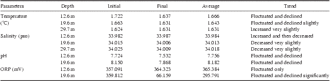
Variations in environmental factors such as water temperature, salinity, pH, and ORP at the time of the arrival of the 2011 Japan tsunami are shown in Fig. 4. Changes in these parameters during the first 48 hours are summarized in Table I. When combined with the sea level oscillations, the figures for water temperature and salinity, especially in the middle and bottom layers, became similar to those of the whole water column. The temperature at the depth of 19.6 m fluctuated and declined slightly from 1.663°C to 1.631°C (-0.032°C). In contrast, the temperature at the depth of 29.7 m increased very slightly from 1.624°C to 1.631°C (+0.007°C). Temperatures became the same after 48 hours. Salinity at these two depths was very similar and showed a slight decrease within 48 hours of the arrival of the first wave. The salinity at 19.6 m decreased from 34.015 to 34.006 psu, and that at 29.7 m decreased from 34.025 to 34.009 psu. The difference between these two layers was only 0.003 psu 48 hours after the arrival of the first wave. The pH at both 12.6 and 19.6 m fluctuated and decreased significantly. The ORP at 12.6 m fluctuated around 350 mV. That at 19.6 m fluctuated and declined significantly to the minimum of 66.159 mV.

Fig. 4 Variations in environmental factors between 10 and 17 March 2011. a. Temperature, b. salinity, c. pH, and d. oxidation-reduction potential (ORP). Variations recorded within the first 48 hours of detected oscillations are shown in the rectangle (the data used for these charts were averaged for each single hour to produce smooth lines).
Table I Variations in seawater parameters during the first 48 hours after the detection of the 2011 Japan tsunami. ORP = oxidation-reduction potential.

Discussion
Several methods have been applied to tsunami detection. Tsunamis can be measured by bottom pressure recorders (e.g. Bernard et al. Reference Bernard, González, Meining and Mulburn2001, Rabinovich et al. Reference Rabinovich, Stroker, Thomson and Davis2011) or satellite altimeters (Okal et al. Reference Okal, Piatanesi and Heinrich1999, Smith et al. Reference Smith, Scharroo, Titov, Arcas and Arbic2005, Ablain et al. Reference Ablain, Dorandeu, Le Traon and Sladen2006) in the open ocean. Tide gauges are the common means of tsunami detection in the coastal waters (Titov et al. Reference Titov, Rabinovich, Mofjeld, Thomson and González2005, Brolsma Reference Brolsma2005, Zhang et al. Reference Zhang, Huang and Wang2008), though other methods such as coastal GPS stations are also used (Song Reference Song2007). Here, we firstly used data from an online mooring system to analyse the influence of teletsunami on Antarctic coastal waters. In this study, spectra used for tsunami analysis and comparative spectra were found to be very similar and no differences in the level of similarity between Ati and A2, or Ati and A3 (or between Bti and B2, or Bti and B3) were found. This shows the validity of the mother wavelet. Compared to upper layer recording data, the oscillations detected in the bottom were visibly lower but the difference was almost negligible (1.3 mm for the 2010 Chile tsunami and 1.7 mm for the 2011 Japan tsunami). These differences might have been caused by movement of the underwater floats fixed on the top of the mooring. However, the data recorded by CTD pressure sensors were credible and the tsunami signal was easily distinguishable from background noise.
The travel speed of the 2010 Chile tsunami to East Antarctica was similar to that reported in other places (c. 190 m s-1, Saito et al. Reference Saito, Matsuzawa, Obara and Baba2010), however, the maximum wave height of 84.4 mm was much lower than that recorded in the coastal waters of China during the 2010 Chile tsunami (20–32 cm, Yu et al. Reference Yu, Yuan, Zhao and Wang2011). The direction of energy propagation might be the main cause of this. The highest wave always reached the site later than the first wave, around 11 hours later in the case of the of 2011 Japan tsunami and a considerable 27 hours later in the case of the 2010 Chile tsunami. The results of analysis of the 2004 Sumatra tsunami suggested that, contrary to near-field regions, the highest tsunami waves arrived several hours to one day after the initial tsunami (Titov et al. Reference Titov, Rabinovich, Mofjeld, Thomson and González2005). The study shows that the duration of the 2010 Chile tsunami in Antarctic coastal waters was around 71 hours and that of the 2011 Japan tsunami was around 58 hours. Such prolonged “ringing” could be explained by persistent incoming wave energy.
This study showed that the Japan tsunami lead to much more profound water level oscillations than the Chile tsunami even though the epicentre of the Chile earthquake was much closer to the observational site. Comparing with the data recorded in the bottom layer, the maximum height of the Japan tsunami in Antarctica was 180.8 mm, similar to that at Cape Roberts in the western Ross Sea (Antarctica) obtained with NOAA models (c. 20 cm, Brunt et al. Reference Brunt, Okal and MacAyeal2011), and more than double the height of the Chile tsunami. The difference could be explained by the following factors: 1) the M w of the Japan earthquake was higher than that of the Chile earthquake, and the epicentre of the Japan earthquake was in the open ocean while that of the Chile earthquake was nearer to the coast, and 2) there were differences in the directionality of energy propagation. The direction of the 2011 Japan tsunami was south-east, exactly the direction of the detection site. However, the direction of the 2010 Chile tsunami is north-west, away from the detection site. It is interesting that the two spectra of depth recorded before the Japan tsunami (11–27 February 2011) were not as smooth as comparable spectra. Fluctuations of c. 5 mm were found around one month before the tsunamis hit. In contrast, smooth spectra were recorded before and after the Chile tsunami.
The weather patterns between 12 and 14 March 2011 showed no evidence of either frontal passages or atmospheric gravity waves. The air temperature from 12–14 March varied between -0.9°C and 3.2°C with an average of 0.6°C. The wind speed ranged from 0–13 m s-1 with an average of 4 m s-1 but usually remained below 5 m s-1. Consequently, sea level perturbations recorded at the Great Wall bay can be linked to the tsunamis. The maximum wave height was 180.8 mm in this study, which was lower compared with those observed in the coastal waters of low latitude. However, it would promote the mixing of sea waters temporarily. The temperature declined and the salinity increased in the upper layer, however, in the bottom layer, temperature increased slightly and salinity decreased, which suggests the occurrence of the mixture of sea waters in the whole water column. Forty-eight hours after the initial wave of the 2011 Japan tsunami reached the Great Wall bay, differences in salinities at depths of 19.6 m and 29.7 m dropped to only 0.003 psu and the temperatures became the same (Table I). This demonstrated that sea level oscillations associated with the tsunami temporarily increased the level of mixing of seawater in the shallow Antarctic coastal waters and influenced the water properties.
Acknowledgements
We thank the members of all the expeditions who helped to deploy the monitoring system in Antarctica's Great Wall bay. This work was supported by the National High Technology Research and Development Program of China (Program 863, No. 2007AA09Z121), the National Ocean Public Benefit Research Foundation (No. 200805095) and the National Nature Science Foundation of China (No. 41076130). The constructive comments of the reviewers are also gratefully acknowledged.