


Introduction
The high elevations of the McMurdo Dry Valleys show a range of ground ice conditions, including dry permafrost, massive ground ice and ice-cemented ground (Campbell & Claridge Reference Campbell and Claridge2006, Bockheim et al. Reference Bockheim, Campbell and McLeod2007, Marinova et al. Reference Marinova, McKay, Pollard, Heldmann, Davila, Andersen, Jackson, Lacelle, Paulson and Zacny2013). The term ‘dry permafrost’ refers to soils with temperatures that never rise above freezing but contain virtually no ice. The only known occurrence of dry permafrost is in the high elevations of the McMurdo Dry Valleys (Bockheim et al. Reference Bockheim, Campbell and McLeod2007). For example, a detailed dataset from Linnaeus Terrace in Upper Wright Valley (1600–1650 m) indicates that the thickness of the active layer is 12.5 cm, the dry permafrost extends to a depth of 25 cm and ice-cemented soil is present below that level (McKay et al. Reference McKay, Mellon and Friedmann1998).
In Beacon Valley at an elevation of ~1400 m there is massive glacial ice buried under 20–50 cm of fine grain material (Sugden et al. Reference Sugden, Marchant, Potter, Souchez, Denton, Swisher and Tison1995). This material appears to be glacial till left behind from the evaporation of the ice. There is some uncertainty about the age of the ice but estimates range from 2–8 m.y. (Sugden et al. Reference Sugden, Marchant, Potter, Souchez, Denton, Swisher and Tison1995, Gilichinsky et al. Reference Gilichinsky, Wilson, Friedmann, McKay, Sletten, Rivkina, Vishnivetskaya, Erokhina, Ivanushkina, Kochkina, Shcherbakova, Soina, Spirina, Vorobyova, Fyodorov-Davydov, Hallet, Ozerskaya, Sorokovikov, Laurinavichyus, Shatilovich, Chanton, Ostroumov and Tiedje2007). However, calculations of the rate of evaporation of this ice using atmospheric temperature and humidity data suggest that it would not persist over millions of years (Hindmarsh et al. Reference Hindmarsh, van der Wateren and Verbers1998, McKay et al. Reference McKay, Mellon and Friedmann1998). These calculations assumed that, in the absence of snow on the surface, the relative humidity (RH) of the surface of the soil was equal to the RH in the atmosphere ~1 m above the soil surface. Schörghofer (Reference Schörghofer2005) and Kowalewski et al. (Reference Kowalewski, Marchant, Levy and Head2006) speculated that the ice may be maintained by variations in climate from present conditions, in particular high values of the atmospheric RH.
In University Valley (77.868°S, 163.758°E, elevation 1700 m, shown in Figs 1 & 2) the depth to ice-cemented ground varies down the valley (McKay Reference McKay2009, Marinova et al. Reference Marinova, McKay, Pollard, Heldmann, Davila, Andersen, Jackson, Lacelle, Paulson and Zacny2013), and recent work by LaPalme et al. (Reference LaPalme, Lacelle, Pollard, Fisher, Davila and McKay2017) also indicates that the ice table characteristics within University Valley are variable across polygon structures. McKay (Reference McKay2009) suggested that the frequency of recurrence of snow on the surface could stabilize the ground ice against evaporation and explain the variation in depth down the valley. This followed the observation at lower elevations by Hagedorn et al. (Reference Hagedorn, Sletten and Hallet2007) who studied ice-cemented ground in Victoria Valley (elevation 450 m) and found that summer snow cover reduced and even reversed evaporation of the ground ice.
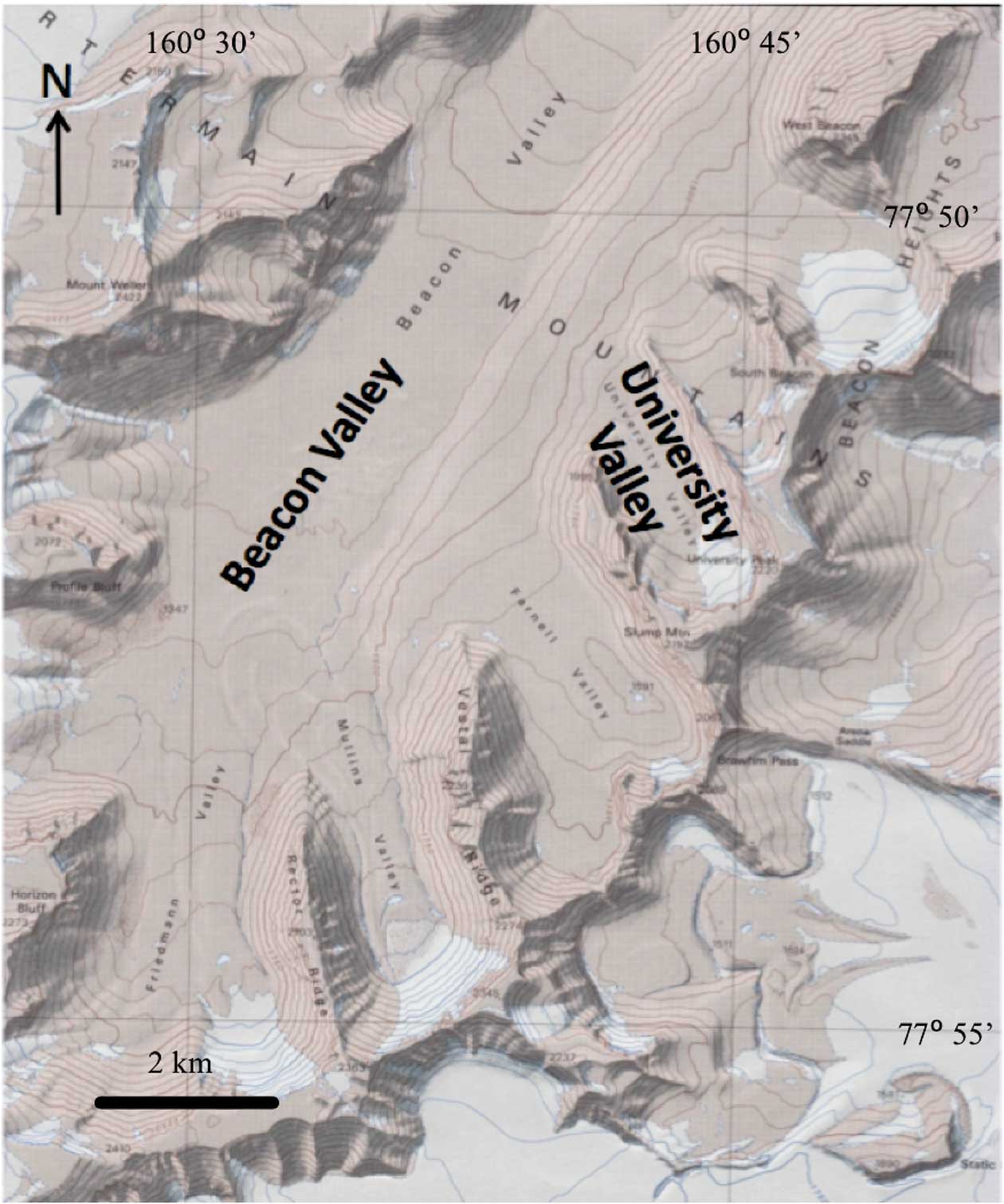
Fig. 1 Map showing University Valley.
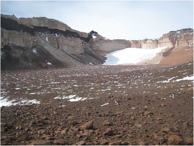
Fig. 2 Photograph of glacier remnant at the head of University Valley, Antarctica in January 2010, facing SSE. The meteorological station used in this study is located mid-valley, slightly down-valley from where the photograph was taken. Width of glacier remnant is ~1 km.
Several lines of evidence suggest that the ground ice is not sublimating as rapidly as the atmospheric models indicate. Ng et al. (Reference Ng, Hallet, Sletten and Stone2005) determined sublimation rates based on nuclides in Beacon Valley cobbles released from the massive ice and found rates that were more than a magnitude smaller than atmospheric models predict. Similarly, Lacelle et al. (Reference Lacelle, Davila, Pollard, Andersen, Heldmann, Marinova and McKay2011) used gradients in the water isotopes in the ground ice to infer sublimation rates in University Valley several orders of magnitude smaller than the atmospheric models predict. Finally, Mellon et al. (Reference Mellon, McKay and Heldmann2014) demonstrated a correlation between the variation in depth to ground ice in University Valley and variation in polygon size and concluded that the present depth distribution of ground ice in this valley has persisted for ~104 years.
The suggestion that the atmospheric models do not correctly predict the boundary conditions at the top of the soil surface was confirmed by Fisher et al. (Reference Fisher, Lacelle, Pollard, Davila and McKay2016). They found that if they set the soil RH fraction to a constant value of 0.85, compared to 0.5 for the atmosphere, ground ice would be stable in University Valley.
In this paper we present model results that further investigate the role of enhanced moisture at the soil surface. We expand on previous work by including more detailed physics. We have a detailed model that is driven by field observations of the atmospheric conditions and compare with measurements of the surface. In particular, we consider physical mechanisms that might be responsible for a higher RH within the pores of the soil surface layer than in the atmosphere 1–2 m above the surface. We focus on two effects: i) retention of water by salt solutions and ii) periodic surficial snow deposits.
Meteorological data
A weather station was deployed in the approximate centre of University Valley (77°51.729'S, 160°42.606'E; elevation 1677 m) in November 2009. A full year of data was downloaded in December 2010. All instruments functioned nominally and data collection was successful. Data were collected at 30 minute intervals and stored with a Campbell CR1000 data logger. Instrumentation on the Campbell weather station included the following.
Campbell 207 temperature and humidity probe
The probe uses a thermistor to measure a wide range of temperatures (~-50°C to +60°C) with a relatively small margin of error (<0.4°C). The RH accuracy is typically better than 5% over the entire RH range. A Campbell 207 probe is mounted 1.2 m above the ground to measure ambient air temperatures. Additional Onset HOBO temperature (-40–70°C,<0.5°C accuracy) and RH (±2.5% accuracy) sensors were placed in the subsurface at depths of surface, 20 cm (about the start of the permafrost) and 42 cm (start of the ice-cemented ground). For temperatures below freezing the RH is corrected to reflect the humidity over ice (e.g. Hagedorn et al. Reference Hagedorn, Sletten and Hallet2007). Note, however, the soil sensors/data were not used in this modelling study given that the soil column variables were calculated via our model. In order to simulate hypothetical snowfall events, the soil surface temperature and RH had to be calculated/modelled.
R.M. Young wind monitor
This wind monitor measures wind speed and direction. The wind monitor can measure wind speeds ranging from 0–60 m s-1 (130 mph). These measurements are necessary to characterize the atmospheric conditions at the field site.
LI200X pyranometer
This pyranometer measures incident solar radiation using a silicon photovoltaic detector. The LI200X operates over a wavelength range of ~400–1100 nm. The LI200X is mounted on the meteorological station 1.27 m above the ground surface to measure incoming solar radiation.
The specific meteorological dataset used in this study covered the date range of 10 December 2009 to 9 December 2010. For model runs where multiple years were required, the year of data was simply repeated. The limitations of this approach are addressed in the Discussion.
Model description
In this study, we attempt to address the question of how the ice table may be affected by boundary conditions by constructing a soil model that includes seasonal thin snow deposits at the surface as well as the presence of different types of salt within the soil pores. The model specifics are given below. Model parameters chosen for the soil are shown in Table I.
Table I Model parameters used for this study.

Soil and snow model
The soil model is similar to that of Williams et al. (Reference Williams, McKay and Heldmann2015) with several exceptions. Briefly, the soil model is a 1-D finite-volume mass and energy model which permits liquid and vapour refreezing within pores. Like many numerical models which track both energy and mass evolution, the model employs a time-splitting technique whereby (for a given time step) the energy of the domain is computed first and then the mass evolution. Appendix 1 contains additional soil column details, as well as the mass flux calculations used in the present model. The soil model uses adaptive time stepping, where time steps are typically 0.1–10 seconds in length, whereas the upper boundary condition of the soil column is determined by the atmospheric data which changes every 30 minutes. Thus the model tracks the water liquid, vapour and temperature profiles in the soil column throughout each modelled day and is capable of resolving very short timescale processes. In this present work we model only vapour diffusion (not diffusion-advection), since the effects of diffusion-advection are insignificant for Earth conditions (Ulrich Reference Ulrich2009). Layer thicknesses were chosen to be 2 cm for this model with an overall soil column of 15 m being simulated. A domain of 15 m was considered sufficient given that the annual thermal skin depth is ~2–3.5 m for the thermal conductivities of dry to icy soil (discussed below). The soil column is shown graphically in Fig. 3.
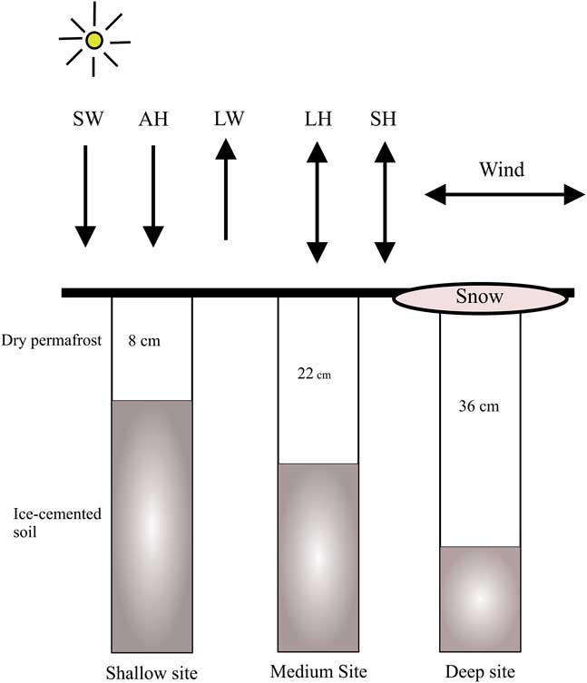
Fig. 3 Diagram of the 1-D soil model. Incoming insolation (SW), outgoing infrared (LW), infrared atmospheric heating (AH), sensible heat (SH) and latent heat (LH) are shown. The snow layer (in this case over the ‘deep’ site) can be placed over any of the three sites when required. The energy balance applies regardless of the surface type (soil or snow).
Three permafrost scenarios were studied. A shallow dry permafrost scenario, designated ‘shallow’, corresponded to 8 cm of dry permafrost overlaying ice-rich soil. For the ‘medium’ and ‘deep’ scenarios, 22 cm and 36 cm of dry permafrost overlaying ice-rich soil were used, respectively. The three depths were chosen to correspond to the considerable down-valley variation in dry permafrost depths which has been measured in University Valley (McKay Reference McKay2009, Marinova et al. Reference Marinova, McKay, Pollard, Heldmann, Davila, Andersen, Jackson, Lacelle, Paulson and Zacny2013).
Soil thermal conductivity was varied between a minimum of 0.6 W mK-1 for dry soil (McKay et al. Reference McKay, Mellon and Friedmann1998) and a maximum of ~2.5 W mK-1 when the soil pore space is completely ice-saturated. The variation between these two values was a function of the pore ice content and calculated in a semi-empirical manner as detailed in Williams et al. (Reference Williams, McKay and Heldmann2015). Consequently, the thermal conductivity of each soil layer changed over time (diurnally, seasonally) as ice entered and exited the soil pores.
The mass diffusivity of water vapour in air was varied as a function of temperature in the manner of Hall & Pruppacher (Reference Hall and Pruppacher1976):
 $$D_{v} \,{\equals}\,2.11 \cdot 10^{{{\minus}5}} \left( {{T \over {273.15}}} \right)^{{1.94}} {{1013.25} \over P},$$
where P is the annual average pressure at the meteorology station (815 mb). The work of Fisher et al. (Reference Fisher, Lacelle, Pollard, Davila and McKay2016) assessed the effects of wind pumping on ice table depth (vs ordinary molecular diffusion) in the Antarctic Dry Valleys and found that the effect is negligible; hence, only molecular diffusion was considered within the interior of our soil column model.
For some model situations salt is permitted within soil pores of the top 4 cm of soil. The depth limit of 4 cm was chosen in accordance with the observation that salt preferentially accumulates in the topmost portion of the soil column; salts are believed to accumulate on the surface from snow condensation nuclei left after sublimation, then salt migration within the soil column is possible depending on water content (Bockheim Reference Bockheim1982, Campbell et al. Reference Campbell, Claridge, Campbell and Balks1998). When salt presence is required in the model, NaCl, CaCl2 or Ca(ClO4)2 was allowed. The presence of salt within pores of a given layer modifies the efflorescence/deliquescence characteristics. For NaCl, the saturation vapour pressure is reduced by 30%, for CaCl2 the reduction is 65% and for Ca(ClO4)2 the reduction can be >80% (Nuding et al. Reference Nuding, Rivera-Valentin, Davis, Gough, Chevrier and Tolbert2014). If present, the brine in the pores is treated as an ideal solution and the freezing point depression calculated as:
 $$\Delta T\,{\equals}\,K_{F} \,bi,$$
where K F =1.853 K kg mol-1 is the cryoscopic constant for water, b is the molality of the solution and i is the Van’t Hoff factor (i=2 for NaCl and i=3 for CaCl2 and Ca(ClO4)2). The mass fractions for salt in the soil was set at 75 µg kg-1, in accordance with the findings of Kounaves et al. (Reference Kounaves, Stroble, Anderson, Moore, Catling, Douglas, McKay, Ming, Smith, Tamppari and Zent2010), where calcium perchlorate salts were measured in the top 10 cm soil in University Valley. We found, however, that our model findings were relatively insensitive to the mass fraction of salt, as there were very small amounts of liquid water/ice in the pores. Only small amounts of water in the pores resulted in extremely briny solutions, which in turn yielded maximal freezing point depressions. Since calcium perchlorate has complex efflorescence and deliquescence properties varying between 5–55% (Nuding et al. Reference Nuding, Rivera-Valentin, Davis, Gough, Chevrier and Tolbert2014), we examined a salt scenario where the deliquescence and efflorescence RH was 20% and the eutectic point 206 K, parameter values which characterize highly soluble hygroscopic salts and in our model represent the effects of magnesium and calcium perchlorate.
The lower portion of the soil column consists of ice-cemented soil. This specification is reasonable since the ground ice observed along the valley floor of University Valley is primarily pore ice (Lacelle et al. Reference Marinova, McKay, Pollard, Heldmann, Davila, Andersen, Jackson, Lacelle, Paulson and Zacny2013, Marinova et al. Reference Lacelle, Davila, Fisher, Pollard, DeWitt, Heldmann, Marinova and McKay2013). The upper portion consists of dry permafrost. Water vapour diffuses in and out of the dry permafrost, occasionally condensing/freezing. Pore volumes for each layer are allowed to evolve depending on ice and water content. If specified, a snow layer is emplaced at particular dates/times at the surface and allowed to sublimate or melt according to the requirements of the snow surface energy balance.
The snow properties considered in the model include snow albedo, density and layer thickness. If a snow layer is present, the soil layer immediately adjacent has a water vapour boundary condition specified to be saturated (i.e. the RH is specified to be 100% with respect to ice). If that soil layer has salt present in the pores, the RH at saturation is scaled (reduced) to the appropriate amount (specified previously in this model description section). We vary snow density as beginning with 60 and 120 kg m-3, given that the density of newly fallen snow varies between 60–120 kgm-3 for dry snow falling in moderate winds (Jordan et al. Reference Jordan, Albert and Brun2008). Varying the snow density for a given snow depth is used to model a range of snow mass loading on the surface (snow mass per unit area). The results of increasing the high snow density in the model up to 200 kg m-3 was analysed as well to test model sensitivity to higher snow density.
Surface energy balance
The soil model has an upper boundary condition specified via the surface energy balance, which in turn is driven by the data gathered from the meteorology station deployed in University Valley. For our finite-volume approach, the energy of the surface layer is evolved by the following expression for the flux across one volume side (of unit area) of the element:
 $${{\partial U} \over {\partial t}}\,{\equals}\,{\minus}k{{\partial T} \over {\partial z}}\left{\Big |} _{{{\vskip -5pt Bottom}} } \right.{\plus}(1{\minus}A)\,S{\minus}{\varepsilon}\,\sigma \,T^{4} {\plus}A_{H} {\plus}SH{\minus}L\,{{\partial M} \over {\partial t}},$$
where U is the energy of the volume element, A is albedo, S is incoming solar shortwave radiation, t is time, T is temperature, M is the convective mass loss (or gain), SH is the sensible heat loss (or gain), AH is the atmospheric heating, L is latent heat and εσT 4 is the outgoing infrared energy. In our model, the emissivity ε was varied depending on the exposed surface. For University Valley, Tamppari et al. (Reference Tamppari, Anderson, Archer, Douglas, Kounaves, McKay, Ming, Moore, Quinn, Smith, Stroble and Zent2012) classified the soil as sandy loam at depths up to 19 cm; hence for bare soil an emissivity of 0.928 was chosen, as used in Mira et al. (Reference Mira, Valor, Boluda, Caselles and Coll2007) as suitable for sandy loam. For snow an emissivity of 0.97 was set (Bonan Reference Bonan1996).
The atmospheric heating term was calculated in the manner suggested by Jordan et al. (Reference Jordan, Andreas and Makshtas1999) as follows:
 $$A_{H} \,{\equals}\,{\varepsilon}\,\sigma \,{\varepsilon}^{{\asterisk}} T_{a} ^{4} ,$$
where ε* is the sky emissivity, which is expressed in terms of cloud cover as:
 $${\varepsilon}^{{\rm {\asterisk}}} \,{\equals}\,0.765{\plus}0.22N^{3} .$$
For cloud cover fraction N. For our purposes the cloud cover fraction was calculated as either 1.0 or 0.0, with the threshold chosen for full cloud cover when the RH was >80% and insolation was <2 W m-2.
The heat conduction to and from the soil layer directly below the soil surface layer is given by:
 $$k\,{{\partial T} \over {\partial z}}\left{\Big |} {_{{Bottom}} } \right.,$$
for the thermal conductivity k. As mentioned previously, the thermal conductivity of each model layer changes as a function of time as mass enters and exits the soil pores. The specific heat capacity and bulk density of a given layer changes with time as well. The internal energy (and hence temperature) evolution of the layer takes into account the time-varying nature of these thermophysical properties.
The sensible and latent heat (mass loss/gain) terms were calculated in conventional bulk aerodynamic flux forms as shown in Appendix 2. When required by the energy balance, frost was permitted to form at the soil surface (albedo was then scaled up to a maximum of 0.35 in a manner described in Williams et al. Reference Williams, McKay and Heldmann2015). In practice, however, the presence of surface frost had a negligible effect in our University Valley model. The frost was too ephemeral, often disappearing within an hour or two of initial formation.
Model results
A set of model runs was completed for each of the three model configurations based on initial ice table depth (shallow, medium and deep). To calculate an ice table recession rate, the model was run for 5–10 years before an annual recession rate was estimated in order to fully initialize the ground vapour and temperature profile. The results are shown in Tables II–IV. Note that the assumed ice in this model is pore ice, not massive ice. The ice table recession rate is not identical to ice mass loss rates, since the variable porosity and pore ice occupancy levels of up to 90% must be taken into account for each layer. The numbers shown here are ice table recession rates, which are calculated as a mass-scaled estimate for a given soil layer. Meteorology station measurements used to drive the ground model are shown in Fig. 4. An example of the modelled snowfall timing and thickness (applicable for some of the model configurations, indicated in Tables II–IV) are shown in Fig. 5.
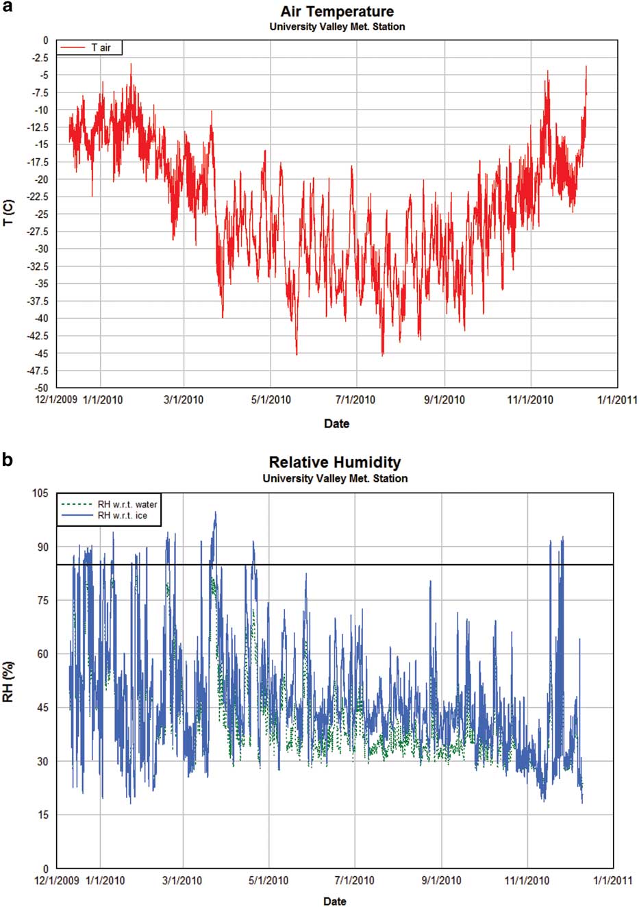
Fig. 4a Air temperature (T) and b. relative humidity (RH) measurements with respect to water (green line) and ice (blue line) obtained at the University Valley meteorological station. The black line in b. indicates 85% RH.
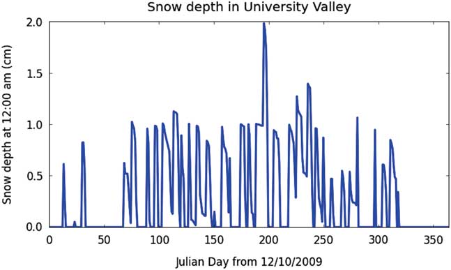
Fig. 5 Modelled snow thickness, in this example for the shallow site, with a snow density of 60 kg m-3. In all of the model snowfall scenarios the snowfall frequency was 1 cm of snow deposited once per week at 00h00. Note that a thin snow deposit occasionally lasts until the next snow deposition event, causing the overall snow thickness to exceed 1 cm. Warmer temperatures cause the thin snow to rapidly sublimate during the warmer months (Julian days ~0–70 and ~320–365).
Table II Model results for the ‘shallow’ ice table scenario. An asterisk (*) indicates that a perennial ice layer formed within the soil surface (depth 0–4 cm), where ‘ice layer’ is defined to be a soil layer containing at least 2% pore ice by volume. A positive sign (+) indicates a net gain in ice at the ice table.

Table III Model runs for the ‘medium’ site. An asterisk (*) indicates that a perennial ice layer formed within the soil surface (depth 0–4 cm), where ‘ice layer’ is defined to be a soil layer containing at least 2% pore ice by volume. A positive sign (+) indicates a net gain in ice at the ice table.

Table IV Model runs for the ‘deep’ site. An asterisk (*) indicates that a perennial ice layer formed within the soil surface (depth 0–4 cm), where ‘ice layer’ is defined to be a soil layer containing at least 2% pore ice by volume. A positive sign (+) indicates a net gain in ice at the ice table.

A baseline model run, where no snow was ever emplaced on the surface, resulted in fairly rapid ice table recession rates in the shallow site (1.90 mm a-1) and moderate loss rates of 0.54 and 0.28 mm a-1 from the medium and deep sites, respectively. Weekly emplacement of a thin (1 cm) snow layer of low density (60 kg m-3), which lasted usually only a few days, resulted in lower ice table recession rates. For example, the shallow site recession rate was reduced by ~33%, the medium site reduced by ~ 39% and the deep site by ~50%.
Emplacement of successively denser snow layers, while keeping snowfall thickness at 1 cm and frequency of one event per week, resulted in sharply reduced recession rates. In the case for the deep site, a snow density of 120 kg m-3 almost completely arrested the ice table recession (and a slight increase of snow density resulted in a gain of ice, i.e. a reduction of the ice table depth). A similar pattern of lower loss rates was seen in the medium and shallow sites. The modelling scenarios where ice table depths grew shallower (and, in some cases, to build up on the surface) are modelling end-member cases; such scenarios are not expected to be representative of actual conditions in University Valley.
While modelled low-density snow deposits sublimate typically within days, the weekly emplacement of denser snow deposits in the model results in persistent surface snow for large periods of the year, providing a sustained humidity source for the upper boundary condition of the soil column. These model results are consistent with observations in University Valley that the snow in polygon troughs, snowfields and snow patches appears to change little in extent throughout the year, though some of the snow persistence in such cases may be due to shadowing. Moreover, the modelled (weekly) snowfall schedule is consistent with snowfall observations in University Valley, where there is no apparent seasonality to snowfall (Liu et al. Reference Liu, Sletten, Hagedorn, Hallet, McKay and Stone2015). Snow deposition can, and does, occur at essentially any time of year. Some snow deposition events are snowfall (actual precipitation events) and others are the result of windblown snow coming from surrounding areas. The salient characteristic for snowfall amounts is the snowfall mass loading, or the product of the density and the snowfall depth. Hence the model does not depend on the snowfall depth details, since we consider a range of snow densities.
The presence of salts in the soil surface layers appears to have opposite effects to the presence of snow deposits. The cases where no snow was emplaced but salt was present resulted in slight increases in the ice table recession rate. In these cases, the presence of salt near the soil surface reduces the RH in the soil layer directly below the salt, resulting in a higher loss rate of the ice table than would have occurred with just the atmosphere alone.
The results show that NaCl distributed in the top 4 cm of soil only slightly increased the ice table recession on all three sites (e.g.~2% at the shallow site). While snow alone reduced ice table loss rates, the presence of both NaCl and periodic snowfall still resulted in substantially reduced ice table loss rates compared to the bare soil case. Salts which were more hygroscopic, however, such as CaCl2 and Ca(ClO4)2, together with snow cover resulted in actually higher ice table loss rates than the bare soil scenarios.
It is of particular interest that the presence of salt in soil layers near the surface frequently results in ‘seasonal’ ice accumulation within those layers in the model. Moreover, in many cases shown in Tables II–IV there are ‘perennial’ ice deposits resulting from combinations of salt and snow. In those cases, there was still ice table recession at the original front (at the original ice table), but a significant ice presence formed in the topmost soil layers. It should be noted that the ice table mass loss at depth was less than the ice gain in the top soil layers; the top soil layers were gaining ice from the atmosphere (and, if present, the overlying snow layer), resulting in a total ice net gain for the entire soil column. This result is consistent with the hygroscopic nature of salt. The presence of salts severely reduces the saturation vapour pressure for the soil layers, causing preferential condensation and freezing within those layers. The small amounts of salt present in our model resulted in only very low molality values within the salty soil, which in turn produced very small freezing point depressions (typically <1°C); hence liquid brines were rarely present in the salty soil layers during the model runs.
In Fig. 6 the results for four cases are shown: i) no periodic snow deposits, ii) salt presence, iii) periodic snow presence and iv) both salt presence and periodic snow. In Fig. 6a there is no snow or salt and the ice table recession rate is relatively high. In Fig. 6b there is salt mixed in the top portion of the soil column, in which case the ice table recession rate is slightly higher than shown in Fig. 6a. In Fig. 6c the ice table recession rate is lowest (and in some cases effectively zero). In Fig. 6d the recession rate is either low (NaCl) or high (CaCl2 and Ca(ClO4)2) compared with the bare soil case shown in Fig. 6a.
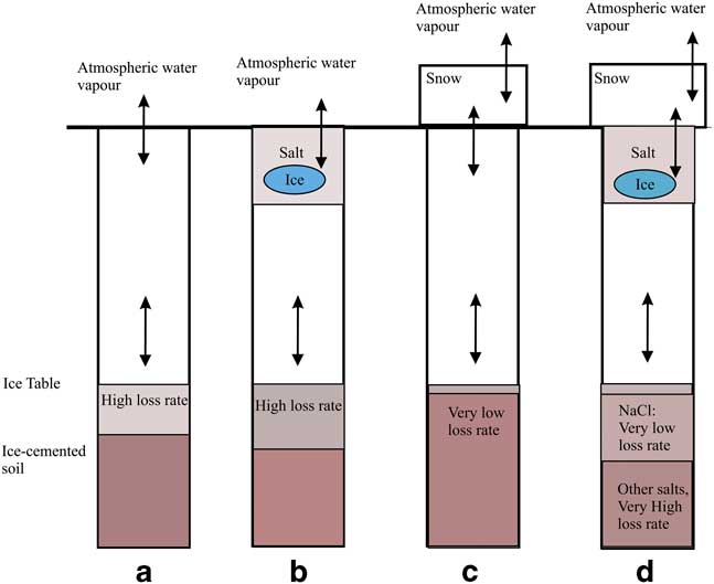
Fig. 6 Ice table recession trends. In a. there is no snow or salt. In b. there are salt deposits within soil pores at the top of the soil column, slightly increasing the ice table recession rate and causing small amounts of ice to form within the pores of the salty soil. In c. and d. there are periodic snow deposits at the surface, slowing the ice table recession rate significantly. In d. there is both snow and salt, resulting in larger amounts of ice forming within the soil surface layer and either a very low ice table loss rate (NaCl) or a high loss rate (CaCl2 and Ca(ClO4)2).
Discussion
While this model is not a detailed prediction of University Valley soils, the amounts observed of ice-cemented ground, ice and salt are within the range of predictions of the model over the environmental parameters that characterize the valley. As mentioned previously, the meteorological data year of 2009–10 was used to drive the model for multiple year runs. The strictest interpretation of the model results would be that the results are only valid for that single year of data. Another shortcoming of this commonly used approach is the apparent incongruity of data on time boundaries: the air temperature at 00h00 on 10 December 2009 is not necessarily close to (or consistent with) the air temperature measurement at 23h00 hrs on 9 December 2010 (the end of the next year). No model snow was laid down during such transitions and the soil model proved to be relatively insensitive to very short-term fluctuations in temperature and RH; the considerable lag (8, 22 or 38 cm) buffers the ice table very efficiently from short-term transients in the atmosphere.
Our model does not include adsorption of water (typically monomer-scale thicknesses) onto soil grains, which may have interesting effects on the water vapour and temperature profiles. Modelling such effects would be a non-trivial exercise given the complicated relationship between binding energies of the liquid monomers onto grains of different mineral types (with characteristic mean specific surface areas) requiring empirical equations to be determined for particular soils. In our model, we neglect physical adsorption of water based on the analysis of Hagedorn et al. (Reference Hagedorn, Sletten and Hallet2007), where they state that changes in the amount of adsorbed water vapour would be small compared to the changes in pore ice.
The findings of Fisher et al. (2016) in University Valley have shown that setting the upper RH boundary condition for the soil model to 85% RH effectively arrests the ice table recession. As a test for our model, we too were able to nearly eliminate ice table recession when setting the same upper boundary condition. But in addition, we find that including a physical mechanism that rationalizes the higher surface humidity, such as thin frost or salt, also reproduces the result of Fisher et al. (2016). In addition, our bare soil model produces loss rates similar to that of Kowalewski et al. (Reference Kowalewski, Marchant, Head and Jackson2012) for polygon centres under 50 cm of soil, where they calculate a loss rate of 0.02 mm a-1 and we calculate a loss rate of 0.05 mm a-1.
The presence of surficial snow deposits evidently contributes to diffusive recharging of the ice table in the Antarctic Dry Valleys. While surface frost was included in the present model, it proved to have no effect on the ice table recession rate. Unlike frosts on Mars at the Viking Lander 2 site, which were comparatively long-lived (Svitek & Murray Reference Svitek and Murray1990, Williams et al. Reference Williams, McKay and Heldmann2015), modelled frosts in University Valley were extremely thin (microns) and too fleeting to have an effect on the ice table recession rate. Snow deposits, given their high albedo and considerable mass, are apparently much more effective at controlling the ice table recession rates.
Salt deposits in soil pores near the surface appear to provide a countervailing influence to that of snow. Additionally, when salt is present in the upper soil column, small amounts of pore ice form near the soil surface. Other salt species or combinations not considered in the present work may play an important role. While sulfate salts have limited solubility, nitrate salts exhibit solubilities intermediate to NaCl and CaCl2 (see Mellon & Phillips Reference Mellon and Phillips2001, fig 7 and references therein). The abundance of nitrates in the regolith is common (Claridge & Campbell Reference Claridge and Campbell1977, Bockheim Reference Bockheim1982) and can in places have abundances comparable to those of chlorides.
The ice table in the Martian high latitudes is expected to be similarly recharged via thin seasonal H2O frost deposits (e.g. Mellon & Jakosky Reference Mellon and Jakosky1993, Mellon et al. Reference Mellon, Feldman and Prettyman2004, Chamberlain & Boynton Reference Chamberlain and Boynton2007, Williams et al. Reference Williams, McKay and Heldmann2015). During the Martian winter, surface temperatures typically dip below the atmospheric frost point inducing surface frost formation. Such frost was observed at the Viking and Phoenix landing sites (Svitek & Murray Reference Svitek and Murray1990, Smith et al. Reference Smith, Tamppari, Arvidson, Bass, Blaney, Boynton, Carswell, Catling, Clark, Duck, DeJong, Fisher, Goetz, Gunnlaugsson, Hecht, Hipkin, Hoffman, Hviid, Keller, Kounaves, Lange, Lemmon, Madsen, Markiewicz, Marshall, McKay, Mellon, Ming, Morris, Pike, Renno, Staufer, Stoker, Taylor, Whiteway and Zent2009). The formation of this frost causes drying of the near-surface atmosphere and effectively pins the humidity boundary condition (Mellon & Jakosky Reference Mellon and Jakosky1993). Salts within the Martian soil may contribute to a similar effect to the Antarctic case. The observed dry permafrost thickness via neutron spectroscopy and in situ excavation is consistent with the predicted depth of ground ice (Mellon et al. Reference Mellon, Feldman and Prettyman2004, Reference Mellon, Arvidson, Sizemore, Searls, Blaney, Cull, Hecht, Heet, Keller, Lemmon, Markiewicz, Ming, Morris, Pike and Zent2009), when it is assumed the atmospheric humidity is about twice the observed value averaged thousand-year timescales. The effects of salts as discussed here would possibly complicate the situation for Mars, where the surface frosts would again provide a recharging effect on the ice table but the salts a desiccating effect.
Conclusion
We have constructed an ice table model which includes both surficial salt deposits as well as periodic snow cover. The model boundary conditions are driven by data taken in the 2009–10 season in University Valley, Antarctica. Our findings suggest that: i) modelled ice table ablation rates in University Valley are strongly affected by seasonal snow cover, ii) ablation computed by the model can be effectively eliminated by snow cover, as has been previously suggested, iii) the addition of salt within the soil pores of the topmost 4 cm of the soil column can have an opposite effect to that of snow cover (i.e. salt in the soil can slightly increase ice table ablation rates), and iv) the 200 year effects of the presence of different amounts of salt within the topmost 4 cm of the soil column can include persistent pore ice within the salty soil layers.
Acknowledgements
This study was supported by NASA’s Planetary Geology and Geophysics Program through grant NNX14AE01A. We thank two anonymous reviewers for their helpful comments on the paper. Any use of trade, firm or product names is for descriptive purposes only and does not imply endorsement by the US Government.
Author contributions
KEW contributed text and wrote the numerical model. JLH contributed text and the data used to drive the model. KEW and CPM designed the study. CPM contributed text. MM contributed text and modelling advice.
Appendix 1
The following is an overview of the mass flux portion of the soil model. The modelled soil column is composed of 750 soil layers (2 cm each), where the top layer is directly exposed to the atmosphere (or snow cover). The soil column is 15 m which is roughly four times the annual temperature skin depth for the highest thermal conductivity material (ice). The upper boundary condition is the time-varying atmospheric measurements of temperature and RH, as well as the solar forcing and horizontal wind. The lower boundary condition is pinned at the depth-adjusted mean annual surface temperature.
Each model layer can exchange water vapour with the neighbouring layers according to thermodynamic requirements. The molar flux (kg-mol/(m2 s)) between a given layer and a neighbour is calculated as:
 $$N_{{H_{2} O}} \,{\equals}\,D_{v} \,{\theta \over \tau }\,{P \over {RT}}\,{1 \over {\Delta z}}(y_{{z1}} \,{\minus}\,y_{{z2}} ).$$
Here the y terms are the water vapour mole fractions at point z1 and z2. The mass diffusivity of water vapour in air is denoted by Dv, soil porosity θ and tortuosity τ. Ambient pressure is P, R is the specific water vapour constant and temperature is T. Except for R and τ, the remaining variables can change in time and space as ice and water vapour move vertically in the soil column. When snow is present at the surface, the surface albedo increases as a function of snow thickness, and the RH is set at 100% for a boundary condition of the topmost soil layer. In this case the topmost soil layer gains ice mass, which affects the thermophysical properties of the layer, and hence the computed temperature.
Each model layer contains variable quantities of liquid water, water vapour and solid ice within the soil pores. The mass fractions of water in different phases within the soil pores depends on the salt efflorescence/deliquescence effects described earlier in the model.
Energy transport is calculated in a flux-conservative form as detailed in Williams et al. (Reference Williams, McKay and Heldmann2015). The temperature for each layer is then diagnosed from the internal energy of each soil layer.
Appendix 2
The turbulent bulk aerodynamic sensible heat term was calculated as:
 $$SH\,{\equals}\,0.4^{2} \,\rho _{m} \,u(z){{T(z_{H} )\,{\minus}\,T(z)} \over {\left[ {{\rm In}\left( {{z \over {z_{M} }}} \right){\rm {\plus}\psi }_{M} } \right]\left[ {{\rm In}\left( {{z \over {z_{H} }}} \right){\rm {\plus}\psi }_{H} } \right]}}.$$
The latent heat/mass loss term is calculated in a manner similar to the sensible heat, and is omitted here for brevity. In the above, 0.4 corresponds to the Von Karman constant, ρ m is the molar density of air, and z is the instrument height. The momentum roughness length z M was estimated to be 0.01, as work by Lancaster (Reference Lancaster2004) found similar values for similar terrain in the Antarctic Dry Valleys. Here the heat roughness length scale zH was assumed to be 0.2z M (as recommended in Campbell & Norman Reference Campbell and Norman1998).
In order to calculate the atmospheric stability (and the corresponding profile diabatic correction factors Ψ M and Ψ H ), it was necessary to first calculate the bulk Richardson number Rib (which is a finite-difference approximation of the ratio of buoyancy to mechanical shear):
 $$R_{{ib}} \,{\equals}\,{{gz{\rm \Delta }\theta } \over {\bar{T}u^{2} }}.$$
Here g is gravity, z is the instrument height, u is the wind speed,
 $${\rm \Delta }\theta \,\approx\,T_{a} \,{\minus}\,T_{{sfc}} ,$$
 $$\bar{T}\,{\equals}\,{{T_{a} {\plus}T_{{sfc}} \over 2}},$$
where Ta and Tsfc are the temperatures in the air and at the surface, respectively.
Once Rib was known, it was possible to calculate the Monin-Obukhov length scale L, the friction velocity u* and the potential temperature scale θ* (Jacobson Reference Jacobson1998):
 $$u^{{\rm {\asterisk}}} \,{\equals}\,{{0.4{\rm }u(z)} \over {{\rm ln}({z \over {z_{M} }})}}\sqrt {G_{M} } ,$$
 $$\theta ^{{\rm {\asterisk}}} \,{\equals}\,{{0.4^{2} u(z)(T_{a} {\minus}T_{{sfc}} )} \over {u^{{\rm {\asterisk}}} Pr_{t} ln^{2} ({z \over {z_{M} }})}}G_{h} ,$$
for the turbulent Prandtl number Prt=0.95, corresponding to a Von Karman value of 0.4. Here the functions Gm and Gh are calculated:
 $$G_{m} \,{\equals}\,1{\minus}{{9.4{\rm }R_{{ib}} } \over {1{\plus}{{70{\rm }(0.4^{2}) \sqrt {\left| {R_{{ib}} } \right|{z \over {z_{m} }}} } \over {ln^{2} ({z \over {z_{m} }})}}}}\;\;\;R_{{ib}} \leq 0,$$
 $$G_{h} \,{\equals}\,1{\minus}{{9.4{\rm }R_{{ib}} } \over {1{\plus}{{50{\rm }(0.4^{2}) \sqrt {\left| {R_{{ib}} } \right|{z \over {z_{m} }}} } \over {ln^{2} ({z \over {z_{m} }})}}}}\;\;\;R_{{ib}} \leq 0,$$
 $$G_{m} ,G_{h} \,{\equals}\,{1 \over {(1{\plus}4.7{\rm }R_{{ib}} )^{2} }}\;\;\;R_{{ib}} \geq 0.$$
The Monin–Obukhov length scale can then be estimated directly:
 $$L\,{\equals}\,{{(u^{{\rm {\asterisk}}} )^{2} \overline{{\theta _{v} }} } \over {0.4g\theta ^{{\rm {\asterisk}}} }},$$
where the average potential virtual temperature in the boundary layer is estimated from the surface temperature Tsfc and air temperature Ta as:
 $$\overline{{\theta _{v} }} \,\approx\,{{Ta{\plus}Tsfc} \over 2}.$$
Once L is known, the stability parameter is defined as:
 $$\zeta \,{\equals}\,z\,/\,L.$$
The profile diabatic correction factors are then calculated as (Campbell & Norman Reference Campbell and Norman1998):
 $${\eqalignno & {\rm \Psi }_{H} \,{\equals}\, {\minus}2\,\ln \left[ {{{1{\plus}(1{\minus}16\zeta )^{1/2} } }} \over 2 \right]\,{\rm and}\,\,\Psi _{M} \,{\equals}\,0.6\,\Psi _{H} \atop \;\;\; \cr & \qquad\quad\quad\quad\quad\quad\quad\quad{\rm \,\,\,\,\,\,for}\,{\rm unstable}\,{\rm flow}\,\zeta \,\lt\,0,\qquad$$
 $$\hskip-38pt{\rm \Psi }_{M} \,{\equals}\,{\rm \Psi }_{H} \,{\equals}\,6{\rm ln}(1{\plus}\zeta )\;\;\;{\rm for}\,{\rm stable}\,{\rm flow}\,\zeta \,\gt\,0.$$


