


Introduction
The McMurdo Dry Valleys of Antarctica comprise the largest ice-free area on the Antarctic continent. They are important for the study of life in extreme environments (Priscu & Christner Reference Priscu and Christner2004), as a physical analogue for Mars (McKay et al. Reference McKay, Andersen, Pollard, Heldmann, Doran, Fritsen and Priscu2005), and potentially as a source of information about ancient Earth climates (Sugden et al. Reference Sugden, Marchant, Potter, Souchez, Denton, Swisher and Tison1995). Soil temperature and water are critical variables affecting soil biological activity in the Dry Valleys (Virginia & Wall Reference Virginia and Wall1999). Buried ice has been found in the Dry Valleys but its age is controversial (Sugden et al. Reference Sugden, Marchant, Potter, Souchez, Denton, Swisher and Tison1995, Hindmarsh et al. Reference Hindmarsh, van der Wateren and Verbers1998, Ng et al. Reference Ng, Hallet, Sletten and Stone2005). The buried ice could be important for reconstructing past climates. The rate of vapour transport through overlying till provides one approach for estimating ice age, but published models for soil temperature and water in the Dry Valleys (e.g. Hindmarsh et al. Reference Hindmarsh, van der Wateren and Verbers1998, McKay et al. Reference McKay, Mellon and Friedmann1998, Schorghofer Reference Schorghofer2005, Kowalewski et al. Reference Kowalewski, Marchant, Levy and Head2006, Hagedorn et al. Reference Hagedorn, Sletten and Hallet2007) are deficient because they do not deal mechanistically with exchanges between soil and atmosphere, and do not treat soil water dynamically.
Doran et al. (2002a, 2002b) analysed meteorological records from the McMurdo Dry Valleys for the period 1986–2000 and found significant declines in summer air temperature, cloudiness and wind speed. The first trend would be expected to decrease summer soil temperature, and the latter two trends to increase it. Thus it is not obvious whether trends in summer soil temperature will follow those in air temperature.
The objective of our research was to construct a mechanistic model of soil temperature and water, specific to the McMurdo Dry Valleys. The model was intended to be applicable for examining abiotic controls of soil biological activity, for predicting soil temperature and water at sites with only standard meteorological observations, and for estimating the rates of water fluxes for various scenarios of soil water content and climate. These objectives required a model that mechanistically treats the processes of heat and water fluxes within soil and between soil and atmosphere.
Literature
Sugden et al. (Reference Sugden, Marchant, Potter, Souchez, Denton, Swisher and Tison1995) estimated the age of buried ice in Beacon Valley, an Antarctic Dry Valley, at 8.1 million years based on argon dating of overlying ash deposits. If the buried ice is as old as the ash, this provides important evidence about the ancient Antarctic climate (Sugden et al. Reference Sugden, Marchant, Potter, Souchez, Denton, Swisher and Tison1995, Marchant et al. Reference Marchant, Lewis, Phillips, Moore, Souchez, Denton, Sugden, Potter and Landis2002). The preservation of ancient ice would imply a low rate of sublimation loss. Estimates of sublimation rates based on the depth distribution of cosmogenic noble gases in till overlying old ice are as low as c. 0.005 mm yr-1 (Schäfer et al. Reference Schäfer, Baur, Denton, Ivy-Ochs, Marchant, Schlüchter and Wieler2000, Marchant et al. Reference Marchant, Lewis, Phillips, Moore, Souchez, Denton, Sugden, Potter and Landis2002, Ng et al. Reference Ng, Hallet, Sletten and Stone2005). Physical models of vapour transport through till under current climate conditions (McKay et al. Reference McKay, Mellon and Friedmann1998, Schorghofer Reference Schorghofer2005, Kowalewski et al. Reference Kowalewski, Marchant, Levy and Head2006, Hagedorn et al. Reference Hagedorn, Sletten and Hallet2007) have yielded higher sublimation rates (0.1–0.5 mm yr-1) assumed to be incompatible with the preservation of ancient buried ice. However, several of these models treat only frozen soil or deal only with summer conditions. None of the models treat sensible heat exchange and vapour exchange between the soil surface and the atmosphere. Several of the models assume a linear gradient of water vapour pressure through the soil from the surface down to the buried ice, and thus implicitly assume that capillary water is in equilibrium with an assumed vapour pressure gradient. Schorghofer & Aharonson (Reference Schorghofer and Aharonson2005), examining ice distribution on Mars, constructed a model similar to that of Kowalewski et al. (Reference Kowalewski, Marchant, Levy and Head2006), but which included equations for soil water content (“adsorbed water”). They concluded that the inclusion of adsorbed water in their model was unimportant for estimates of the relationship between the atmospheric concentration of water vapour and the depth and amount of buried ice, as long as the adsorbed water was in local equilibrium with an assumed linear gradient of water vapour pressure in the soil profile. Several authors (Hindmarsh et al. Reference Hindmarsh, van der Wateren and Verbers1998, Schorghofer Reference Schorghofer2005) have acknowledged that it is necessary to treat the relationship between soil water and vapour pressure to estimate ice sublimation rates, but none have examined seasonal variation of capillary water under the influence of atmospheric driving variables, or the disequilibrium in vapour pressure gradient attending periodic water input to the soil.
Materials and methods
We adapted models to three terrestrial sites (Table I), each free of permanent ice and within a few metres of ice-covered Lakes Bonney, Hoare or Fryxell in Taylor Valley, Antarctica (Priscu Reference Priscu1999, and other articles in Bioscience Volume 49, No. 12). Doran et al. (Reference Doran, Dana, Hastings and Wharton1995) described meteorological instrumentation at the sites, and data can be found online at the McMurdo Dry Valleys Long Term Ecological Research project site (http://mcmlter.org/queries/met/met_home.jsp, accessed October 2009). Many of these data, up to the year 2000, were analysed by Doran et al. (Reference Doran, McKay, Clow, Dana, Fountain, Nylen and Lyons2002a). For present purposes, the data were divided into sets used for model calibration and for validation tests (Table I).
Table I Site characteristics of meteorological stations (Doran et al. 2002a), and datasets used for model tuning or validation.

Simulation model
The energy model incorporates concepts of energy fluxes at a bare soil surface, based on the model of Matthias (Reference Matthias1990). Components of the energy budget include net radiation (Rn), sensible heat (H), latent heat (LE) and soil heat conduction (G). All these components of the surface energy balance are functions of surface temperature. In the model of Matthias (Reference Matthias1990) and many other energy balance models, the value of a theoretical surface temperature (Tsfc) is estimated iteratively to achieve a balance among the processes adding and removing energy from the surface. That is, a constant Tsfc is estimated so that:
The rates of processes at the equilibrium Tsfc are then assumed to apply over the time interval for which the driving variables are averaged, typically 24 hours. We took a slightly different approach, for reasons explained below.
Because the McMurdo Dry Valleys are rocky, the surface layer is divided into rock and soil fractions with different thermal properties. Furthermore, a fraction of the surface may be covered with snow. Thus our model includes three different surface temperatures: for rock, soil, and snow. To calculate sensible heat exchange with the atmosphere as a function of surface temperature, we used the area-weighted average temperature of rock, soil and snow. In an early version of the model, we tried the above approach of Matthias for estimating equilibrium Tsfc, but found that the iterative procedure solving simultaneously for three surface temperatures was complicated, computationally inefficient and not reliably stable. Therefore we replaced the concept of a boundary surface temperature with that of the temperature of a thin (0.5 cm) surface layer. Rather than solving for instantaneous steady state values of the surface layer temperatures (Tr1, Ts1, and Tw1 for top layers of rock, soil, and snow, respectively), the energy fluxes were allowed to operate over short (much less than one day) time intervals, and temperatures were updated as a function of surface layer heat contents and heat capacities. Using this approach of a thin surface layer, surface temperatures approached steady state values within a fraction of a day, using driving variables that were constant over a day. The model was dynamically stable with this solution technique.
Net radiation in the model is the sum of incoming shortwave, reflected shortwave, incoming longwave, and emitted longwave radiation, each calculated separately for rock, soil, and snow surfaces. Incoming shortwave radiation (Wm-2) observed at Taylor Valley sites is a driving variable. Reflected shortwave radiation is predicted from the albedos of rock, soil (Table II) and snow. Snow albedo is assumed constant (0.90) at all sites. Incoming longwave radiation (Rl) is predicted from air temperature Ta (K), following Matthias (eq. (8), 1990):
Table II Site specific parameters of the simulation model.

1Fallow field at Yuma, Arizona, USA (Matthias Reference Matthias1990).
where εc is atmospheric emissivity and σ is the Stefan-Boltzmann constant (5.67 x 10⁻⁸ W m-2 K-4). Atmospheric emissivity εc is calculated as a function of Ta and cloud cover (eqs (9) & (10) in Matthias Reference Matthias1990). Cloud cover cf is estimated from observed incoming shortwave radiation Rs and estimated maximal incoming shortwave radiation Rsm.
Maximal radiation Rsm as a function of season was estimated by fitting empirical curves to maximal radiation observed over an approximately ten year period (Fig. 1). The curves vary among sites because of shading from mountains in the Asgard Range (Dana et al. Reference Dana, Wharton and Dubayah1998). These estimates of cloud cover might also be affected by unobserved variations in atmospheric transmissivity.
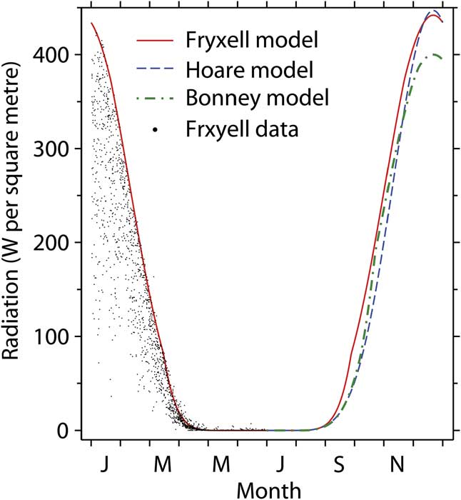
Fig. 1 Average daily incoming shortwave radiation at Taylor Valley sites. Observed radiation at the Fryxell site is shown for the first six months. The lines are for modelled maximal radiation.
Longwave radiation emitted from the ground surface is predicted from Eq. (2), substituting surface layer temperatures Tr1, Ts1, or Tw1 for Ta, and using the corresponding emissivities of rock, soil and snow in place of εc. Snow emissivity εw was estimated to maximize the fit to data. The value of εw varies among sites (Table II), but stays within the range for snow and ice given by Hori et al. (Reference Hori, Aoki, Tanikawa, Motoyoshi, Hachikubo, Sugiura, Yasunari, Eide, Storvold, Nakajima and Takahashi2006). We developed an equation for soil emmisivity εs as a function of surface temperature TCs1 (°C), applicable between -40 and 15°C, based on data of Wan (http://www.icess.ucsb.edu/modis/EMIS/images/goleta2.prn, accessed November 2006) for beach sand:
where m1 is a site-specific multiplier (Table II), and εs is constrained to be < 1.0. Multiplier m1 is 1.0 for the data of Wan (as above). Rock emissivity εr is assumed to depend on temperature according to Eq.
(4)with site-specific multipliers m1 as given in Table II.
Sensible heat exchange between the atmosphere and surface layer is formulated as in Matthias (eqs (12)–(17), 1990), except that his eq. (15) for the heat exchange coefficient under unstable conditions, Chu, is replaced by the following corrected equation (Matthias, personal communication 1 November 2006, see also Mahrt & Ek Reference Mahrt and Ek1984):
where Chn is the coefficient under neutral conditions, and Co is a function of instrument height. The bulk Richardson number Ri is calculated using eq. (13) from Matthias (Reference Matthias1990), replacing his values of surface roughness and surface temperature with area-weighted averages of the rock, soil and snow surfaces (Table II). The critical value of Ri, above which laminar flow ensues, is 0.2, in the middle of the range of literature values given by Matthias (Reference Matthias1990).
Latent heat flux in the surface layer is predicted from freezing/thawing of soil water and from water vapour exchange with the atmosphere and with the second soil layer. Water vapour exchange between the surface soil layer and atmosphere (instrument height = 3 m) is predicted from the humidity gradient and wind speed using an atmospheric transport equation (eq. (5) in Kondo et al. Reference Kondo, Saigusa and Sato1990). The bulk coefficient for water vapour exchange is assumed the same as that for heat exchange as calculated according to Matthias (Reference Matthias1990, see above). Saturation vapour pressure in the atmosphere as an empirical function of temperature is calculated using eq. (6) in Murray (Reference Murray1967). Humidity at instrument height is calculated from saturation humidity and relative humidity. In soil air, water vapour pressure is assumed to be in local equilibrium with ice or capillary water because of the large surface areas and short diffusion distances involved. In frozen soil, soil air humidity is the same as that over ice at the predicted soil temperature. In unfrozen soil, vapour pressure is calculated from soil water matric potential (assuming zero osmotic potential) using the Kelvin equation. Matric potential is estimated as a function of soil texture, bulk density and volumetric soil water using a water-release equation formulated for sandy soils typical of the McMurdo Dry Valleys (eq. (4) in Hunt et al. Reference Hunt, Treonis, Wall and Virginia2007), assuming 4.4% clay, 90.5% sand, and an average sand particle diameter of 0.28 mm. Soil bulk density is assumed to increase with depth (Table III). Water vapour exchange and latent heat flux in the top layer of snow is calculated using the same equations as for soil, except that the relative humidity of air in the snow is assumed to be 100%. Vapour exchange between the atmosphere and wetted rock surfaces is not considered.
Table III Ground layer properties in the simulation model.

Snow cover was estimated as a function of albedo, calculated from incoming and reflected shortwave radiation. There was a regular seasonal pattern at all three sites (except in midwinter when low light precluded calculation), with very high snow cover in spring and autumn and low cover in summer. However, the radiation sensors are at 3 m height, and a fraction of reflected shortwave radiation appears attributable to nearby snowfields, glaciers and ice-covered lakes (Dana et al. Reference Dana, Wharton and Dubayah1998), in addition to local snow at the meteorological stations. We used regression analysis to statistically remove the regular variation in reflected shortwave radiation related to seasonal changes in sun angle in relation to the positions of glaciers and lakes. The residual (local snow cover) was much more variable than the uncorrected estimates, and was generally greater in spring and autumn, and lower in summer, which agrees with field observations. However, using constant snow cover in the model gave a better fit to temperature observations at two of the three sites (Hoare and Fryxell) than using variable snow cover (either corrected or uncorrected for reflection from lakes and glaciers). This suggests that: 1) reflection at 3 m height assesses snow cover over a much larger area than that (presumably < 1 m2) influencing the soil temperature sensors, 2) reflectivity of glaciers and lakes varies importantly between years, or 3) snow depth in addition to snow cover is necessary to predict soil temperature. We compared three snow indicators at the Bonney site based on direct snow depth measurements, observed albedo, and the departure between observed emitted longwave radiation and that predicted from observed soil surface temperatures. There was no useful correspondence among the three indicators. Thus for predicting temperatures, we assigned a constant snow cover (Table II) equal to the annual average corrected snow cover at each site. This assumption is relaxed for some model exercises (below). Seasonal minimum observations of albedo were used to constrain estimates of rock and soil albedo in the model (Table II).
The ground, composed of soil and rocks, is divided into discrete layers to a depth of 10 m (Table III). The rock fraction increases with depth in accordance with information from near the Hoare site (Campbell Reference Campbell2003). Heat capacity of the rocks is set to 1.32 Jg-1 °C-1, within the range for non-porous rocks. Heat flux between adjacent layers is calculated separately for the rock and soil fractions, because of the large differences in thermal conductivities of rock and dry soil. Heat flux between layers occurs only from rock to rock or from soil to soil, on the assumption that rock-soil interfaces do not coincide exactly with interfaces between layers. For both soil and rock, interlayer flux is calculated according to Matthias (eq. (24), 1990), except that the flux is also proportional to the average fraction of soil (or rock) for the two layers. The effect of temperature TC (centigrade) on rock thermal conductivity is based on eq. (3a) in Clauser & Huenges (Reference Clauser and Huenges1995):
where λT is a temperature multiplier, normalized to equal 1.0 at 25°C, for site-specific values of rock thermal conductivity (Table II), A (0.985 J °K-1 m-1 sec-1) and B (863, complex units) are constants estimated to achieve a fit to data in Clauser & Huenges (Reference Clauser and Huenges1995, fig. 2c) for plutonic rocks poor in feldspar (which include granite), and 3.29 is estimated thermal conductivity at 25°C. Soil thermal conductivity is predicted as a function of temperature, gravimetric soil water (liquid and ice) and bulk density. If gravimetric water is > 1%, equations developed by Kersten (Reference Kersten1949) for frozen and unfrozen sands and gravels are used. For drier soils, a constant value (0.24 J °K-1 m-1 sec-1) for quartz sand is used (fig. 2, Buchan Reference Buchan1991). Intra-layer heat conduction between rock and soil is calculated using similar equations as for interlayer flows. The conducting area (surface area of rocks) and the average distance between the centres of rocks and pockets of soil are calculated as a function of layer thickness, fraction of rocks and soil by volume, and by assuming a simple geometry of regularly spaced uniform spherical rocks. The equations require a single new parameter, rock diameter (Table III), assumed invariable across sites. Thermal conductivity for intra-layer heat flux is taken as the weighted average of rock and soil conductivity.

Fig. 2 Simulated temperatures and observed 5 cm depth temperatures at the Bonney site in 2001–02.
The freezing point of capillary soil water is calculated as a function of soil water potential according to Buchan (eq. (34), 1991), assuming zero osmotic potential and zero ice pressure. If the layer temperature exceeds the freezing temperature, ice melts at a rate proportional to the mass of ice, the difference between freezing and layer temperatures, and to an empirical rate constant (10 day-1 °C-1). Varying the rate constant had little effect on temperature dynamics, because freezing and melting are ultimately controlled by heat transfers between layers, which are modelled mechanistically. Latent heat flux is proportional to water frozen or thawed. Freeze/thaw flows are suspended in dry soil (volumetric water < 0.5%) to speed model solution.
The movement of soil water vapour from layer i to layer j, Qvij (m3 sec-1), is calculated from the humidity gradient assuming Fickian diffusion:
where D is the diffusivity of water vapour, ρ is air density, P is air-filled soil porosity, A (m2) is the cross-sectional area of soil between layers, vi and vj are the specific humidity of air in layers i and j, and L (m) is the distance between midpoints of the two layers. Tortuosity is not considered for these sandy soils. Diffusivity D (m2 sec-1) as a function of temperature is predicted according to Kondo et al. (eq. (6), 1990). Air density ρ (kg m-3) is calculated as a function of temperature (Matthias Reference Matthias1990). Air-filled porosity P is total porosity minus the volume of ice and water. Total soil porosity is calculated from bulk density and the specific gravity of solid constituents (Hunt et al. Reference Hunt, Treonis, Wall and Virginia2007). Specific humidity v is calculated as explained above for latent heat flux in the surface layer. Soil water vapour is not a state variable in the model, because its mass will be orders of magnitude less than water or ice. Thus vapour fluxes between layers are handled as exchanges among the state variables for water and ice. For vapour flows involving layers with mixtures of water and ice, the flow is assigned to the predominant phase, which determines the appropriate latent heat fluxes. The balance among ice, capillary water and vapour pressure is then re-established via the freeze-thaw process described above, including latent heat fluxes.
Capillary water flow Qlij (m3 sec-1) from soil layer i to layer j is calculated using Darcy’s law (Fetter Reference Fetter1994):
where K (m sec-1) is hydraulic conductivity (defined below), hi and hj (m) are the hydraulic heads in layers i and j, A is cross sectional area and L is distance between layers. Hydraulic head h is the sum of elevational head (m) and water potential head hp (m), which is calculated from water potential ψ (kPa) (Fetter Reference Fetter1994):
where 1000 converts kPa to Pa (Pa = kg m-1 sec-2), g is the acceleration of gravity (9.8 m s-2) and sg is the specific gravity of water, assumed equal to 1020 kg m-3. Saturated hydraulic conductivity Ks (m s-1) is calculated according to eq. (5) in Rawls et al. (Reference Rawls, Gimenez and Groosman1998):
where constants C (0.000536 m s-1) and D (2.3, non-dimensional) have values appropriate to sand textured soils, and θe is “effective porosity”, defined as total porosity minus volumetric water content at -33 kPa water potential (Rawls et al. Reference Rawls, Gimenez and Groosman1998). Effective porosity is calculated using the water-release equation discussed above (Hunt et al. Reference Hunt, Treonis, Wall and Virginia2007). Unsaturated hydraulic conductivity K is predicted from Ks and matric potential ψ (kPa) using an empirical equation (eq. (1) in Jaynes & Tyler Reference Jaynes and Tyler1984):
where constant β has a value (2.8, complex units) estimated for a sand textured soil (site 10, Jaynes & Tyler Reference Jaynes and Tyler1984), and operator exp(x) denotes ex, with e the base of natural logarithms. To evaluate Eq.
(8), hydraulic conductivity is taken as the average K in layers i and j, and area A is 1.0 minus the average rock fraction in the two layers.
The rates of radiation, heat and water fluxes described above are collected into a set of difference equations for the rates of change of state variables: heat, water and ice in the soil and rock fractions of each of 13 soil layers. The equations are solved using a variable time step chosen to limit the rate of change of the most rapidly changing state variable (typically water in the surface layer) to less than 1% per time step, which gives a satisfactory compromise between execution time and accuracy of integration. At the end of each simulated day the final equilibrated values of simulated longwave radiation and soil temperatures are compared with the observed daily mean values.
Some model parameters (Table II) were estimated, using enhanced SIMPLEX optimization (Hunt et al. Reference Hunt, Antle and Paustian2003), to give the best fit of the model to observed temperature, radiation and degree days. Degree days is the sum of average daily temperature (°C) for days with temperature above 0°C. Moorhead et al. (Reference Moorhead, Wall, Virginia and Parsons2002) found that degree days correlated strongly with nematode population growth predicted by a population model. The fit of our model to degree days was included to improve the prediction of summer temperatures critical to biological activity. The objective function Q minimized by the optimization procedure is:
where DDm is predicted degree days in the third soil layer (3–7 cm), DDd is observed degree days at 5 cm soil depth, and R2i is the coefficient of determination for data type i. For the Bonney site, data included incoming and emitted longwave radiation and soil temperatures at 0, 5 and 10 cm. For the other two sites (Hoare and Fryxell), data included only 5 and 10 cm temperatures.
For each site, data were divided into calibration and validation sets. Site specific parameters (Table II) were estimated using the calibration sets only. Fits to the validation sets tested the predictive power of the model. We attempted to minimize the number of parameters with different values for the three sites. Initial values of soil water and temperature in each layer were arrived at by repeatedly running the model with the calibration set, taking the final values of temperature and soil water as the initial values for the next run, and repeating this process until the final values were close to the initial values. Thus we assumed that the initial values of temperature and water in the tuning runs were not grossly out of equilibrium with the subsequent driving variables. However, these initial values differed from a true model steady state which was found by a different technique described below. Initial values of temperature and water in the validation runs were set equal to the corresponding values for the same day and month in the calibration run.
Statistical models
Regression models were constructed to predict daily average soil temperatures as a function of driving variables. Linear regression models were formulated using BMDP program 1R (Dixon Reference Dixon1985). Variables with tolerance of less than 0.01 were omitted from the equation (coefficients of zero). Regression models were formulated using the same driving variables and distinguishing the same calibration and validation datasets as used for the simulation model. For examining long term trends, we calculated averages for seasonal periods within which there were no missing daily averages over multiple years, to avoid confounding between season and year of measurement. For example, at the Bonney site there were uninterrupted series of data between 17 November and 29 July for eight periods between 1994 and 2005. Within each period, separate averages were calculated for two seasons, demarcated by the average date when average daily temperature at 10 cm depth first dropped below -10°C. At the Bonney site, this date varied over eight years between 23 February and 3 March. Independent variables were the mean Julian dates for the two seasons.
Results
Models
Table II gives site-specific values for seven parameters found to strongly influence the fit of the simulation model to data and to require different values at different sites. Parameter values used in the original model formulation of Matthias (Reference Matthias1990) are included for comparison, and these generally fall within the range for the McMurdo Dry Valley sites, except for rock/soil albedo which is highest at the agricultural site. Our values for albedo of rocks and soil (0.066–0.142) are within the range of 0.061–0.26 given by Campbell et al. (Reference Campbell, MacCulloch and Campbell1997a) for several Dry Valley locations. Figure 2 shows an example of simulated temperature dynamics and fit to data. Temperature at 3 m depth had a mean of -17°C, amplitude of 14°C and minimum daily mean in early October. This compares well to 3 m temperatures observed in Wright Valley (Thompson et al. Reference Thompson, Craig and Bromley1971) which had a mean of -19°C, amplitude of 14°C and minimum monthly mean in September. Table IV gives a quantitative measure of the fit of the simulation model to data. For the tuning sets, the fraction of variation in dependent variable accounted for by the model (R2) ranged from 0.97 to 0.99 for soil temperature. The R2 for incoming and emitted longwave radiation (Bonney site only) were 0.57 and 0.97, respectively. Table V compares observed and simulated degree days. The simulation accounted for 99% of the variation in observed degree days at the Bonney site and 96% at Fryxell.
Table IV Fit (square root of mean squared error) of simulation models to data.

1datasets defined in Table I.
t = tuning Dataset; otherwise a validation set.
Table V Observed and simulated degree days (the sum of daily average temperatures above 0°C) at 5 cm depth. Only summer seasons with complete records are included.

Regression models predicting daily average soil temperature were developed using only the tuning datasets. Table VI gives the regression models and fits to soil temperature data. The models accounted for more than 97% of the variation in soil temperature, and residual error ranged between 1.2–2.3°C. All driving variables of the simulation model contributed significantly to the regression models, except for wind speed at the Hoare site and relative humidity at all sites. The effect of reflected shortwave radiation was inconsistent and did not contribute significantly after incoming radiation was in the equations. The variables “Day” (Julian day) and Day2 were included to force a seasonal pattern. The signs of coefficients were generally consistent across sites and depths.
Table VI Regression models for daily mean soil temperature (°C) and the fit to data for tuning sets.

#R2 is the fraction of variation of the dependent variable accounted for by the regression model.
*SRMSE is the square root of the mean squared error.
The residual errors of regression and simulation models for temperature data and the predictive power of these models were compared using two kinds of statistical tests. In the first (within sites) test, the fit of models to data used for model development (tuning sets) was compared to the fit for data that were from the same site but not used for parameter estimation (validation sets). Seven sets of data (combinations of site and depth) allowed for a balanced ANOVA design for comparing tuning and validation sets. The interaction between model type (regression vs simulation) and dataset was significant, with the regression models fitting better for surface temperature and simulation models fitting better at 10 cm depth. Surprisingly, the fit was not significantly better (P < 0.35) for the tuning sets than the validation sets. Disregarding the distinction between tuning and validation sets allowed the inclusion of two additional datasets (surface temperatures at Hoare and Fryxell). Analysis of all nine datasets confirmed the depth by model type interaction (Table VII). The second (across sites) test evaluated the ability of models to predict temperatures at sites different from the site used for parameter estimation (Table VIII). The regression models better predicted temperatures at the same site used for model development, while the simulation model better predicted temperatures at different sites.
Table VII Residual error (square root of mean squared error, °C) for within site comparisons of simulation and regression models of soil temperature. The model type by depth interaction is significant at P < 0.0001.
Table VIII Residual error (square root of mean squared error, °C) for simulation and regression model predictions of soil temperature at the same site used for model development vs at different sites. The two-way interaction is significant at P < 0.0001.
Long-term trends
Statistical tests for temporal trends at the three sites employed seasonally averaged variables (5cm soil temperature, degree days, 3m air temperature, incoming shortwave radiation, wind speed and albedo) vs date for each of two seasons. Within each site, data were included only for time periods which had no missing daily mean observations over multiple years. There were between four and nine such time periods for different sites between 1994 and 2005. We tested for the significance of temporal trends using analysis of covariance (programme 1V, Dixon Reference Dixon1985) with year as the covariate and six classification groups defined by three sites and two seasons. Mean values of the dependent variables varied significantly with season and site, the latter effect partly attributable to defining seasons differently for different sites. However, the slopes of the covariate (temporal trends) did not differ significantly from zero and did not vary significantly among sites or seasons for any variable. Only wind speed approached significance (P < 0.08) with a decline of 0.40 m sec-1 decade-1. Table V gives predicted and observed degree days (calculated based on average daily temperatures) for years with complete summer season records. Degree days calculated using 15–20 minute intervals yielded 10% greater sums, but results of the two methods were highly correlated (r > 0.998). For the six years with degree day records at both Bonney and Fryxell, ANOVA showed that most of the variation (85%) was associated with site (P < 0.0001), but that year was also significant (P < 0.003). However, linear temporal trends were not significant (P < 0.52) at either site. There were significantly (P < 0.005) more freeze events per year at the Fryxell site (5.0) than at Bonney (2.5), but no significant temporal trends (P < 0.17).
Depth of thaw
Simulated depth of thaw was surprisingly dynamic (Fig. 3), changing as much as 35 cm over a few days. Annual maximal depth of thaw was attained by early January at the Fryxell and Hoare sites, but not until early February at Bonney. Table IX shows estimated maximal depth of thaw for all years under both observed and elevated temperatures. The effect of elevated temperature on depth of thaw at the colder sites was less in absolute terms, but greater in relative terms. To determine the time required for the system to equilibrate to elevated temperatures, we made a ten year model run for the Bonney site using driving variables for 2003–04 repeated year after year. Depth of thaw virtually stabilized by the second season for both observed temperatures (54 cm to permafrost) and elevated temperatures (77 cm to permafrost). Figure 4 shows the depth distribution of degree days for summer seasons at the Bonney site with complete records of driving variables. Degree days declined rapidly with depth - by about 50% in the top ten centimetres. Seasons with similar depth of thaw could have very different degree days in the surface layers (e.g. 1997–98 and 2004–05).

Fig. 3 Simulated daily average depth of 0°C estimated by interpolation between layers for 1996–97. Observed sign changes of daily average temperature at 5 and 10 cm depth are indicated for the Bonney (triangles) and Fryxell (circles) sites.
Table IX Response of simulated maximal seasonal depth of thaw (cm) to elevated air temperature (+2°C).

1Model driven with observed air temperatures.
2Model driven with year-around elevated air temperatures.

Fig. 4 Simulated depth distribution of degree days (0°C base) at the Bonney site for selected years. The model was driven with observed air temperatures.
Energy budgets
Table X shows aggregated energy budgets for the top (0.5 cm thick) layer of rock, soil and snow. The site trend in annual shortwave radiation results mainly from less cloud cover at sites farther from the ocean (Bonney), although shortwave radiation at the Hoare site is also reduced by shading from nearby mountains (Doran et al. Reference Doran, McKay, Clow, Dana, Fountain, Nylen and Lyons2002a). The site patterns in annual net longwave radiation and sensible heat exchange result largely from the trend in surface temperature (Bonney > Hoare > Fryxell). The sum of annual net longwave and shortwave radiation is positive at all three sites, which agrees with estimates from the Wright Valley (Thompson et al. Reference Thompson, Craig and Bromley1971). Both the annual energy balance (net) and the annual net heat conduction between the top two layers are small components of the budget, indicating that the system is near a steady state on an annual basis. Latent heat fluxes are small because the sites are very dry. This may help explain the rapid changes in depth of thaw predicted for the Bonney site (above). At all three sites, longwave radiation caused a net cooling of the surface most of the time. On summer days, the surface lost sensible heat to the atmosphere at a rate comparable to the loss via longwave radiation. As winter progressed, sensible heat exchange declined in absolute value and turned positive after the sun disappeared. Heat conduction between the first and second layers followed a predictable seasonal pattern at all three sites. In summer when the surface layer was heated by shortwave radiation, surface soil temperature usually exceeded rock temperature by up to 3°C (Fig. 5) because the dry surface soil conducts heat more slowly and has a lower heat capacity than rock. Thus in summer, heat was transferred from soil to rock at rates up to 0.5 Wm-2. In winter, surface temperature of soil differed from rock by ± 5–7°C (depending on wind speed and the difference between air and surface temperatures) and heat transfers between rock and soil were ± 10–15 Wm-2. There was a small annual net heat transfer of 0.57 Wm-2 from rock to soil in the surface (0–0.5 cm) layer, but there was little difference between rock and soil temperatures below 3 cm depth.
Table X Simulated surface energy budgets (Wm-2) for the period from 9 July 1996–8 July 1998. Positive flows add heat to the surface layer (0–0.5 cm). The “summer day” was taken as the first day in the spring when average daily soil temperature at 10 cm depth exceeded 10°C (1°C at Fryxell). The first winter day was when 10 cm soil temperature first dropped below -10°C, and the second winter day was when incoming shortwave radiation first fell below 1 Wm-2.


Fig. 5 Simulated surface (0–0.5 cm) temperatures at the Bonney site in 2001–02.
Water budgets
Precipitation in the floors of the McMurdo Dry Valleys appears to be quite low, perhaps about 1.3 cm yr-1 (Beyer et al. Reference Beyer, Bockheim, Campbell and Claridge1999). We did not use the precipitation data available for our sites because these data are difficult to interpret (Harris et al. Reference Harris, Carey, Lyons, Welch and Fountain2007). Most precipitation comes as snowfall, and much of it appears to be lost via sublimation and wind ablation (Campbell & Claridge Reference Campbell and Claridge2006). Thus snow cover does not automatically lead to water input to soil. Table XI gives our estimates of liquid and vapour transfers at the surface. The largest water inputs came from melting snow, which varied among sites from 1.7–3.4 cm yr-1 in proportion to estimated snow cover. Vapour movement from snow to underlying soil was smaller, but was as great as 27% of snowmelt at the Fryxell site. Potential evaporation was simulated by adding a continuous water supply to the top soil layer, but disallowing capillary flow to avoid altering soil heat conduction. Gooseff et al. (Reference Gooseff, McKnight, Runkel and Vaughn2003) estimated open pan evaporation north of the Hoare site for 11 January 2000 as 0.62 cm day-1, which compares well to the model estimate of 0.51 cm day-1 for the Hoare site on the same date. Potential evaporation at these sites was large compared to the simulated rate of snowmelt, and thus there was no water infiltration below the surface layer. Daily fluxes of soil vapour, either upward or downward, had a maximal magnitude of < 0.002 cm day-1. Annual net vapour flux between the surface layer and the underlying soil was upward at the Bonney site, and downward at the Hoare and Fryxell sites.
Table XI Simulated water transfers (cm yr-1) involving the top layer. The transfers were calculated over a unit area of ground (snow, bare soil and bare rock), rather than for bare soil only. Positive transfers add water to the top layer. The model was run for two years beginning 9 July 1996.
1This was estimated by running the model with a continuous input of water to keep the top soil layer saturated.
McMurdo Dry Valley soils may have water contents below 0.1% gravimetric (Hunt et al. Reference Hunt, Treonis, Wall and Virginia2007). Thawed dry soil may have higher water potential than ice, even at low soil water contents (cf. Schorghofer & Aharonson Reference Schorghofer and Aharonson2005). This is illustrated for our model in Fig. 6. The wettest soil is at saturation (zero water potential) and thus freezes at 0°C (assuming zero osmotic potential, as in the present model). The soil with 0.005 g water per gram dry soil freezes at about -15°C, and below that temperature the curve merges with that for the saturated soil, because ice is present in both. The very dry clay soil (6.1% clay, bottom line) has a greater vapour pressure than saturated soil at 0°C if the dry soil is warmer than about 8°C, a value commonly reached in many Dry Valley surface layers. At 1% gravimetric water, soil warmer than 2°C has greater vapour pressure than ice at -25°C for a range of sandy textures.

Fig. 6 Effects of temperature and gravimetric soil water (g water per g dry soil) on specific humidity in soil air. The upper four lines are for a typical McMurdo Dry Valley soil with 95% sand and 2.3% clay. The bottom line is for a soil with 86% sand and 6.1% clay, within the range of variation for the Dry Valleys (Hunt et al. Reference Hunt, Treonis, Wall and Virginia2007). Circles indicate freezing temperatures for the upper three lines. The two driest soils freeze at below -40°C.
Figure 7 shows that simulated water vapour concentrations in summer were high and variably dependent on depth through the top 55 cm of soil, and then declined with depth into the frozen layers. In winter, the gradient was usually reversed with lowest vapour concentrations at the surface. Disruptions of the usual winter pattern (Fig. 7, peaks in the 0–0.5 cm humidity) were correlated with katabatic winds, as observed in Victoria Valley (Hagedorn et al. Reference Hagedorn, Sletten and Hallet2007). Figure 8 shows the complete gradients for selected dates indicated in Fig. 7. The humidity gradients were smaller, in absolute terms, in winter. The depth of the highest vapour concentration varied over time between the surface (27 December) and 7.75 m (15 October), but was nearer the surface (0–50 cm) when the gradients were steepest. In November to February, humidity in the surface layer was appreciably greater than air humidity, which would speed vapour exchange between soil and atmosphere, but slow exchange within the soil. Figure 9 shows daily vapour fluxes between the first two soil layers. Fluxes could be either upward or downward any season of the year, although sublimation was predominantly downward. Evaporation was the predominant process in the top two layers even in winter because these layers were dry and froze only at low temperatures (cf. Fig. 6). Annual net vapour fluxes (Table XII) in the run without irrigation were upward in soil above 22 cm depth and downward below 35 cm. Capillary flows from layer 7 (35–55 cm) to layers 6 and 8 resulted from occasional melting events in layer 7 (Fig. 3). Such meltwater might flow laterally over permafrost (Harris et al. Reference Harris, Carey, Lyons, Welch and Fountain2007). Water losses from the soil exceeded inputs by 0.148 mm after 2 years and 0.57 mm after 4.6 years.

Fig. 7 Simulated dynamics of water vapour for selected soil layers at the Bonney site in 2002–03. Triangles indicate dates for which detailed humidity gradients are presented in Fig. 8.

Fig. 8 Simulated humidity gradients for selected dates at the Bonney site in 2002–03. The values plotted above zero depth are observed air humidity at 3 m. Seasonal dynamics for several depths are given in Fig. 7.

Fig. 9 Vapour fluxes between the first (0–0.5 cm) and second (0.5–3 cm) soil layers at the Bonney site. Positive fluxes are upward. Evaporation and sublimation pertain to conditions in the source layer.
Table XII Simulated effect of a pulse of water on water transfers (mm in two years) in the Bonney profile. In the irrigated run, 10 mm water at 0°C was added instantaneously to the top layer in early summer when the soil surface was thawed. Positive flows are downward.

1Flow between layer 1 (0–0.5 cm) and layer 2 (0.5–3 cm). Bottom of layer (cm) is given in parentheses.
2Includes the 10 mm added water.
To examine the effect of water infiltration below the surface layer, we simulated the instantaneous addition of 1 cm of water to the top soil layer in early summer. Water infiltrated relatively deeply (Table XII) because of the high rock content and low field capacity (c. 0.05 g water per g dry soil) of the sandy soil, but no added water infiltrated below 35 cm. Added water held against gravity in the surface layer was lost by evaporation within two days, and that in the 0.5–3 cm layer within 20 days. In the 3–7 cm layer, added water was largely lost via evaporation and sublimation within 3.5 months (Fig. 10). The 13–22 cm layer retained about 0.03 g water per g dry soil after 4.6 years. Very little of the water which infiltrated below 22 cm was lost after 4.6 years. The soil still retained 0.44 cm of added water two years after irrigation and 0.30 cm after 4.6 years. Water addition raised the level in the profile below which vapour flows were downward, and increased the rates of downward vapour flows (Table XII).
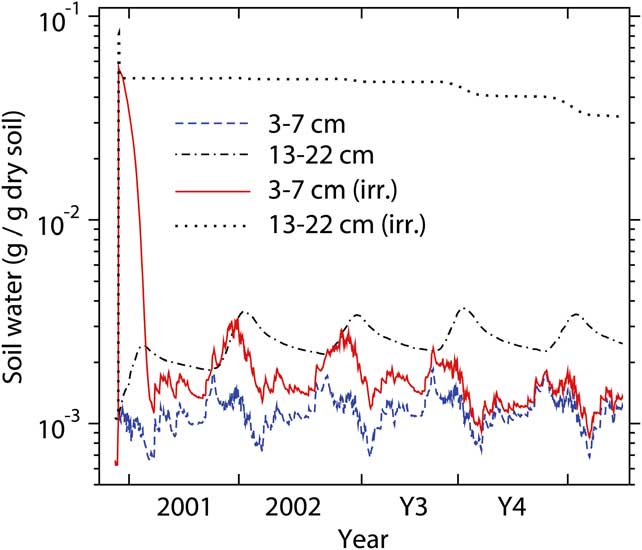
Fig. 10 Simulated effect of a 1 cm irrigation event on soil water dynamics at the Bonney site. The model was run for 2.6 years using observed driving variables, and then another 2.0 years reusing the same driving variables but beginning on the appropriate day and month.
If the model is driven using the same weather variables year after year, soil water eventually will approach a constant depth distribution - a steady state depending on snowmelt and the water vapour content of the atmosphere. Soil water changes so slowly that it was impractical to use simulation to examine the approach of soil water from a completely dry state to the steady state. Instead, we found a series of approximations to the approach to steady state based on the assumption that higher layers equilibrate with the source/sink of water before underlying layers do. This approach showed general agreement with simulation in a 300 year model run starting with a fully saturated profile. Figure 11 shows the approximated approach of soil water to steady state from either dry or saturated initial states. Equilibration to within 2% of steady state occurred much faster beginning from saturation (269 years) than from a dry state (42 000 years).

Fig. 11 The dynamics of the depth distribution of water in two situations beginning with either: 1) dry soil (blue dashed lines), or 2) wet soil (green dot-dashed lines). The steady-state distribution is given by the solid red line with circles, the circles indicating the mid-points of soil layers. Numbers indicate the years required to reach the indicated depth distribution. The last depth distribution shown for the first simulation (blue dashed line indicated by triangle) occurred after 25 208 years, and the last shown for the second simulation (green dot-dashed line indicated by triangle) occurred after 269 years.
Sensitivity analysis
The sensitivity of the simulation model to driving variables and to selected processes and parameters was evaluated using the Bonney model. In Table XIII, the first two indicators of model response (R2 and degree days) were used in estimating parameters, but the second two (depth of thaw and evaporation) were not, because we lacked data for those indicators. Beneath the standard run (first entry in the table), entries are ordered according to absolute departure from degree days in the standard run. Heat exchange between the top 22 cm and the ground beneath had a large effect in cooling surface layers in summer and warming them in winter. Decreasing the roughness length increased sensible heat exchange with the atmosphere and cooled the ground surface in summer, reducing depth of thaw and evaporation. The fraction and properties of rocks had large effects on the model, but we have little information on rock content at the meteorological stations. Among the driving variables, only air temperature appreciably affected degree days or R2. Reducing soil emissivity led to reduced longwave emission and increased soil warming in summer. The above five alterations caused the largest departures for degree days and also tended to cause larger reductions in R2. In the lower portion of the table, all 14 alterations had high R2 and degree days within 15% of the standard run. Nevertheless, maximal depth of thaw in these 14 runs varied from 18–99 cm, and evaporation from 0.0–2.6 cm. Thus wide variation in predictions of evaporation and depth of thaw are compatible with good fits to the temperature data. Campbell & Claridge (Reference Campbell and Claridge2006) identified albedo as a critical variable affecting Dry Valley soil temperature, but increasing albedo from 0.066 to 0.11 in the model had a relatively small cooling effect, because it caused only a 5% decline in absorbed shortwave radiation. Alterations affecting water supply and water fluxes had little effect on temperature because the system is so arid.
Table XIII Simulation model response to altered driving variables and model processes. Results are from a two-year run of the Bonney model beginning 17 November 2000.

1For parameters, standard values are given in parentheses.
2wmin is the value of volumetric soil water below which water fluxes in a layer are suspended to reduce computer run time.
Discussion
The simulation model fitted the observed soil temperature data well, except that the model tended to overestimate surface temperatures in winter by a few degrees. This problem may have resulted from errors in specifying the depth distributions of rocks and water, which control thermal properties, but which were not based on information specific to our sites. Thermal properties of the ground are known to vary across sharp compositional boundaries at some sites in the McMurdo Dry Valleys (Pringle et al. Reference Pringle, Dickinson, Trodahl and Pyne2003). Overestimating winter surface temperatures will have little effect on simulated water vapour transfers because the effect of temperature on water vapour pressure is small below -30°C, and because depth gradients of vapour pressure are smallest in winter. The regression models fitted the temperature data better than the simulation models, at least when applied to the same site used for model specification. This difference probably results from including imperfectly known structures and processes in the simulation model, for example the depth distribution of thermal properties. Of course the regression models do not treat soil water and lack the heuristic value of the simulation model.
Doran et al. (Reference Doran, Priscu, Lyons, Walsh, Fountain, McKnight, Moorhead, Virginia, Wall, Clow, Fritsen, McKay and Parsons2002b) found significant decreases in air temperature and wind speed between 1986 and 2000 at the Hoare site. We found no significant temporal trends for air temperature or soil temperature at any of three Taylor Valley sites including Hoare, although a decline in wind speed was almost significant. However, our analyses were not strictly comparable to theirs because we analysed fewer years and a more recent time period.
Simulated depth of thaw was quite variable within and between seasons. Seasonal maximal depth of thaw at the Bonney site for 2001–02 (79 cm) was somewhat greater than the value of 61 cm estimated for the same site for 2001–02 by Lyons et al. (Reference Lyons, Welch, Carey, Doran, Wall, Virginia, Fountain, Csatho and Tremper2005) using a simple model driven by average annual air temperature. The range of seasonal maximal depth of thaw over sites and years predicted by our model was 18–79 cm. Reported ranges of seasonal depth of thaw based on data from soil pits include 20–100 cm for coastal Dry Valleys (French & Guglielmin Reference French and Guglielmin2000), and 10–65 cm for both coastal and upland sites (Campbell et al. Reference Campbell, Claridge, Balks and Campbell1997b). These studies were not based on multiple observations over dates in late summer, and thus probably underestimate depth of thaw (Campbell & Claridge Reference Campbell and Claridge2006). Moorhead et al. (Reference Moorhead, Wall, Virginia and Parsons2002) suggested that Dry Valley nematode populations require about 50 degree days per year to sustain their populations, and that nematodes are most abundant between 2.5 and 10 cm depth. Our results from the Bonney site indicate that soil below 10 cm would accumulate less than 50 degree days in some (one of eight) years, and that soil above 3 cm could dry (halting nematode activity) within 20 days of being wetted. Thus the model supports the conclusion of Moorhead et al. (Reference Moorhead, Wall, Virginia and Parsons2002) that temperature and water patterns may account for depth distribution of nematodes.
French & Guglielmin (Reference French and Guglielmin2000) cited an estimate by T.J.H. Chinn of 18 cm potential annual evaporation in a coastal Dry Valley region. This is close to our estimate of 19 cm at the Fryxell site, the closest to the coast of our three sites. Our simulated rate of snowmelt was too slow to overcome the high evaporation demand and allow water to infiltrate below the surface layer. Indeed, we have no direct evidence for water infiltration at our meteorological sites for the years studied. The best way to estimate precipitation inputs to soil may be to monitor soil water in surface layers. Kowalewski et al. (Reference Kowalewski, Marchant, Levy and Head2006), applying this method, recorded six soil wetting events at 2 cm depth in one season in Beacon Valley, but they could not quantify the water inputs. Linking such observations to a mechanistic simulation model should allow simultaneous estimates of evaporation, infiltration and vapour fluxes within the soil.
The model predicted a net gain in soil water at the Hoare (0.084 mm yr-1) and Fryxell (0.087 mm yr-1) sites over a two year period, even in the absence of capillary water inputs below the surface layer. At the Bonney site, there was a net loss of 0.074 mm yr-1, which is smaller than the lower range of previous loss estimates predicted from vapour transport. In contrast to previous vapour models for the McMurdo Dry Valleys, our model calculated water vapour pressure in unfrozen soil using a water release curve. Consequently, relatively dry thawed soil could have higher water vapour pressure than ice, and water vapour fluxes in summer were sometimes downward. Another difference from previous vapour models is that we simulated soil water dynamics, and did not assume that soil water is in equilibrium with a uniform depth gradient of vapour pressure. Our results suggest a highly dynamic depth gradient of vapour pressure. At the Bonney site, a single water input of 1 cm persisted well beyond five years and reduced evaporative losses originating from below 22 cm. To wet the soil to 13 cm depth, where added water could persist for three or four years, would require a rapid input (faster than the rate of evaporation) of about 0.26–0.72 cm water to the soil surface (assuming a range of soil textures typical of the McMurdo Dry Valleys, and 50% rock content). Such water inputs every few years would prevent the attainment of any uniform humidity gradient, and reduce or reverse the simulated soil water loss at Bonney.
If soil water happened to be at steady state for a particular year, then annual net change in soil water would be zero. Thus water gains at the Hoare and Fryxell sites indicate that simulated soil water is below the steady state level. Soil water is probably rarely at steady state for any given year because of annual weather variation and because climate shifts faster than soil water can approach a new steady state, which requires hundreds or thousands of years. Thus soil water will track climate with a significant lag. Our results also suggest that glacier ice would persist indefinitely once till accumulates to sufficient depth (100 cm at the Bonney site) at which the ice is in steady state with inputs from snowmelt and exchanges with atmospheric water vapour. On the other hand, water-saturated soil lying below ancient volcanic ash could form at 100 cm depth within 40 000 years via vapour transport through the ash. Our model does not fully address the question of buried ice because it does not include overburden pressure potential or the formation of ice lenses.
Neither our model nor any of the above cited models for estimating sublimation rates include the effects of the high salt concentrations found in some McMurdo Dry Valley soils. Soil salts likely have important effects such as lowering freezing temperatures, increasing soil water contents for a given water vapour pressure, speeding heat conduction in wetter soils, and altering water vapour gradients and vapour fluxes. However, it may be difficult to evaluate salt models because of the lack of data on salts from sites with meteorological stations. Salt composition may vary with depth in complicated patterns (Claridge et al. Reference Claridge, Campbell and Balks1999). Thermodynamic models provide only equilibrium compositions of soil solutions, while rates of dissolution and crystallization are required for any dynamic model of soil salt solutions. Thus a simple empirical approach may be required.
Acknowledgements
Research supported by NSF project OPP-0423595, the McMurdo LTER. Chris Gardner provided quality control for the meteorology data. The reviewers (Kevin Hall and James Head) and editor made useful suggestions for improving the manuscript.


