


Introduction
Zooplankton in the Southern Ocean (SO) are zonally bounded by oceanic fronts, reflecting specific physical requirements that structure their distributions (Atkinson & Sinclair Reference Atkinson and Sinclair2000). Studies in the Atlantic and Indian Ocean sectors of the SO have variously identified the Sub-Tropical Front (STF), Sub-Antarctic Front (SAF), Polar Front (PF) and Antarctic Divergence as separating distinct communities (Atkinson & Sinclair Reference Atkinson and Sinclair2000). These fronts are recognized as important biogeographic boundaries for zooplankton, based on their temperature and salinity characteristics (Deacon Reference Deacon1982). For example, temperature alters the rates of various biological processes in copepods, such as their growth, productivity and mortality (Hirst & Kiørboe Reference Hirst and Kiørboe2002). Differences in environmental factors (physical, chemical and biological) and processes (e.g. stratification, mixing, grazing) define the composition, abundance and productivity of the phytoplankton community (Deppeler & Davidson Reference Deppeler and Davidson2017), and subsequently the zooplankton. Most zooplankton sampling in the SO has been conducted with horizontally towed nets (Hunt & Hosie Reference Hunt and Hosie2003, Takahashi et al. Reference Takahashi, Hosie, McLeod and Kitchener2011), facilitating detection of changes to surface zooplankton community structure (Takahashi et al. Reference Takahashi, Kawaguchi, Hosie, Toda, Naganobu and Fukuchi2010a), seasonal cycles (Hunt & Hosie Reference Hunt and Hosie2006a) and interannual variation (Takahashi et al. Reference Takahashi, Hosie, Kitchener, McLeod, Odate and Fukuchi2010b). To date, there has been little study of the horizontal distribution of zooplankton in the Indian sector of the SO, particularly in the region between 47°E and 57°E. Furthermore, there is little information available on the vertical distribution of zooplankton in the permanent open ocean zone of the Indian sector of the SO. To address this shortage of information, zooplankton were collected between 47°E and 57°E in order to understand the seasonal zooplankton abundance in this region, focusing on species composition and distribution patterns.
The objectives of the present study were to investigate the physical and biological mechanisms that mediate the abundance and distribution patterns of zooplankton communities, paying particular attention to the horizontal and vertical biogeographic patterns in zooplankton community structure in the central Indian sector of the SO east of the Kerguelen Plateau.
Materials and methods
As part of the seventh Indian expedition to the SO, hydrographic and biological measurements were carried out on board Ocean Research Vessel Sagar Nidhi between 40–56°S and 47–57°E (Fig. 1). Sampling occurred between 28 January and 23 February 2013. Temperature and salinity were measured at each station using conductivity-temperature-depth (CTD) profilers (Sea-Bird Electronics, USA). Water samples were collected from ~2–3 m depth using 10 l Niskin bottles attached to the CTD rosette. Water samples from the surface (~2–3 m) for nutrients and chlorophyll a (chl a) were measured following the recommendations of Grasshoff et al. (Reference Grasshoff, Ehrhardt and Kremiling1983) and UNESCO (1994), respectively. The correlation coefficient for NO3-, NO2-, PO3- and SiO44- was 0.9999–1.0000 and for NH4+ was 0.9996–0.9999, with a precision of ± 0.06, ± 0.006, ± 0.01, ± 0.003 and ± 0.005 μM for NO3-, NO2-, NH4+, PO3- and SiO44-, respectively. A total of 5 l of surface water was collected for the pigment analysis. Pigments were separated following slight modifications of the procedure of Van Heukelem (2000), which provides quantitative and qualitative analysis of several phytoplankton pigments. The diagnostic pigment analysis (DPA) was applied to classify phytoplankton types from high-pressure liquid chromatography pigment data (Vidussi et al. Reference Vidussi, Clustre, Manca, Luchetta and Marty2001). Additionally, the Hirata method (Hirata et al. Reference Hirata, Aiken, Hardman-Mountford, Smyth and Barlow2008) was used to refine the DPA in order to separate picoeukaryotes from nanoeukaryotes. With the Brewin method (Brewin et al. Reference Brewin, Sathyendranath, Hirata, Lavender, Baraciela and Hardman-Mountford2010), this relationship and the fraction of each size class were quantified, before the method was applied to the chl a concentration.
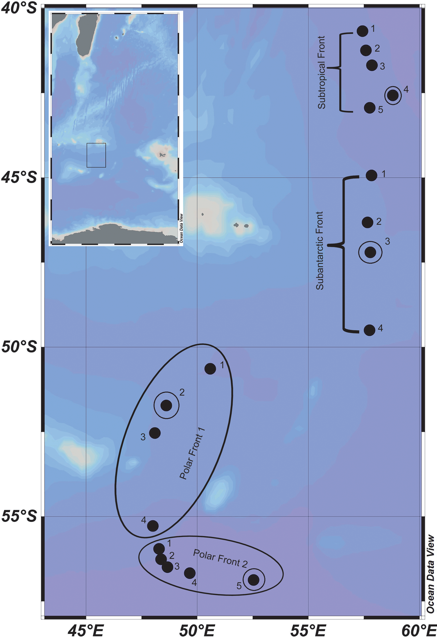
Fig. 1. Study area showing sampling locations (solid dots). The inset image shows a broader map, and the rectangle inside it corresponds to the study area. Small circles indicates vertical sampling points.
Zooplankton samples were collected from the surface (~2–3 m) by horizontal towing of a bongo net (200 μm mesh; net opening 0.32 m2) at 18 stations in the Indian sector of the SO during daylight hours (Fig. 1 & Table SI). The volume of water filtered by the net was measured with a calibrated flowmeter (General Oceanics, USA) mounted in the mouth of the net and used to calculate zooplankton abundances. Following each surface sample, vertical zooplankton samples were collected from four stations (Table SII) in the upper 1000 m from five discrete depth strata using a multiple plankton sampler (MPS; Hydro-Bios, net opening 0.25 m2, mesh size 200 μm) (Weikert & John Reference Weiker and John1981). Two electronic flowmeters were mounted onto the underwater unit in order to calculate the volume filtered. The depth interval of each top stratum was decided based on CTD profiles as follows: surface to the depth of mixed layer (MLD; MLD varied from 40 to 85 m), MLD to 150 m, 150 to 300 m, 300 to 500 m and 500 to 1000 m. The MLD was computed based on the density difference criteria and was considered as the depth at which potential density increased by 0.03 from the 10 m depth value. The MPS was hauled up at a speed of 0.8 m s-1; upon recovery of the samples, the catch was immediately preserved in a 5% buffered formaldehyde/seawater solution. At each station, total catch of each stratum was taken for quantitative biomass analysis. Zooplankton biomass was measured by the volume displacement method (ICES 2000). Large gelatinous plankton such as salps and jellyfish were removed, and salps were identified to family level. When the sample size was large, as was usually the case in the first, second and third strata, it was split using a Folsoms plankton splitter until ~25% of the sample was available for counting and identification of taxa. Often when the numbers in the deeper layers were low, the entire sample was counted and all organisms identified. Specimens were identified to species level for most taxonomic groups, except for Chaetognatha and Appendicularia, which were counted as one taxon each. In order to test for spatial variability in the environmental parameters, analysis of variance was applied. Multiple regression analysis was performed using zooplankton biovolume and abundance as dependent variables and environmental parameters as predictor variables. In addition, the Shannon diversity index (Hˈ) was calculated for the copepod communities.
Results
Variability in temperature and salinity
During the summer of 2013, sea surface temperature varied between 1.14°C and 18.97°C in the study area. Strong temperature gradients occurred between the STF and the PF. Towards the south, a decrease in temperature was noted in PF1 and PF2, while lower temperatures were measured in the PF2 region (Table I). The mean temperatures in the surface waters differed significantly between the frontal regions (P < 0.0001). Small salinity changes occurred at the STF, SAF, PF1 and PF2, and the highest mean salinity in surface waters was observed at the STF (Table I). From 42°S southwards, surface salinity decreased; however, the region between 53°S and 56°S exhibited slightly higher salinity (increase in salinity by 0.06 for PF1 and 0.09 for PF2), but the mean values did not show a significant difference among the frontal regions (P > 0.05). The water temperature was uniform in the mixed layer (MLD) and decreased below MLD. Depth-integrated temperature differed significantly between frontal regions (P < 0.001). The average temperatures within the MLD were 12.20 ± 0.05°C, 7.79 ± 0.08°C, 4.03 ± 0.005°C and 2.43 ± 0.008°C in the STF, SAF, PF1 and PF2, respectively. In the present study, average MLD was 36 ± 25 m in the STF, and increased towards the PF, with the average MLD of 50 ± 18 m in the SAF. In the two most southern sampled areas, the PF1 and PF2 MLD varied between 57 ± 23 m and 76 ± 21 m, respectively.
Table I. Variability in surface temperature and salinity at various frontal regions of the Indian Ocean sector of the Southern Ocean during summer 2013.

STF = Sub-Tropical Front, SAF = Sub-Antarctic Front, PF = Polar Front.
Nutrients and chl a distribution
A southwards increasing trend in nutrient concentrations was observed, with the maximum dissolved inorganic nitrogen (DIN), dissolved inorganic phosphate (DIP) and dissolved silica (DSi) observed at PF2 (Table II). The STF and SAF had lower nutrient concentrations compared to the PF. The highest mean DIN concentration in the surface waters was observed in the PF2 and showed significant difference between the frontal regions (P < 0.001) (Table II). Relatively low phosphate concentrations were observed in the study area; however, significant variations were observed between the fronts (P < 0.05), and the highest concentration was observed in the PF2 (Table II). Regions of higher water temperature coincided with lower silicate concentrations. Furthermore, the mean DSi concentrations were significantly different between the fronts (P < 0.0001), and the highest mean value was observed in the PF2 (Table II). The phytoplankton biomass (chl a) concentration in the surface ranged from 0.08 mg m-3 to its highest values of 0.8 mg m-3 on transect #1 in the PF1, followed by the PF2, STF and SAF (Table III). No significant differences were found among the frontal regions (P = 0.06) (Table III). Overall, there were no significant correlations between chl a and nutrients (DIN, P > 0.6; DIP, P > 0.21; and DSi, P > 0.3) in the study area. During this study, it was observed that diatoms dominated the phytoplankton community structure in the PF1 and PF2 (Fig. 2), where silicate-independent phytoplankton (i.e. small cells) occurred in low numbers. Picoplankton and nanoplankton were dominant in the STF and SAF, respectively (Fig. 2).

Fig. 2. Surface phytoplankton size distributions presented as average percentage contributions to the phytoplankton community at sampling locations a. Sub-Tropical Front, b. Sub-Antarctic Front, c. Polar Front 1 and d. Polar Front 2. The phytoplankton compositions are derived from pigment analysis.
Table II. Variability in surface water nutrients at various frontal regions of the Indian Ocean sector of the Southern Ocean during summer 2013.

STF = Sub-Tropical Front, SAF = Sub-Antarctic Front, PF = Polar Front.
Table III. Average chlorophyll a concentration and variability of zooplankton biovolume and abundance of surface water samples from various frontal regions of the Indian Ocean sector of the Southern Ocean during summer 2013.

STF = Sub-Tropical Front, SAF = Sub-Antarctic Front, PF = Polar Front.
Zooplankton biovolume and abundance
Biovolume and abundance varied spatially, and there were significant differences among the frontal regions (P < 0.05). The mean zooplankton biovolume in the surface layer was high in the PF2, while the lowest was observed in the SAF (Table III). The maximum zooplankton abundance was observed on transect #4 in the PF1 and the lowest was observed on transect #1 in the SAF. Zooplankton biovolume exhibited a significant positive relationship with abundance (r 2 = 0.95; P < 0.001). Zooplankton biovolume (r 2 = 0.52) and abundance (r 2 = 0.61) tended to decrease with increasing temperature. Depth-integrated zooplankton biovolume and abundance in the upper 1000 m at four oceanographic stations ranged from 0.03 to 0.085 ml m−3 (Fig. 3) and from 248 to 1068 ind m−3, respectively; at station 46°58'S, 57°30'E they varied from 0.03 to 0.15 ml m−3 (Fig. 3) and from 156 to 1164 ind m−3. Relatively, southwards increasing trends were observed at station 52°25'S, 48°05'E ranging from 0.08 to 0.22 ml m−3 (Fig. 3) and from 304 to 1682 ind m−3. The highest values were observed at station 56°34'S, 53°39'E ranging from 0.06 to 0.35 ml m−3 (Fig. 3) and from 250 to 2684 ind m−3.

Fig. 3. Vertical variation in zooplankton biovolume at four oceanographic stations. MLD = depth of mixed layer.
Major zooplankton community structure and copepod species composition in the surface layer
Zooplankton in the surface layer included Copepoda, Chaetognatha, Appendicularia and Salpida (Table IV). In this study, copepods were the most important group of zooplankton throughout the transect, consisting mainly of Calanoida and Cyclopoida (Table IV). The mean abundances of calanoids (P < 0.001) and cyclopoids (P < 0.001) in the surface waters differed significantly between the frontal regions. Overall, calanoid copepods were the most abundant group in all of the regions, followed by cyclopoid copepods (Table IV). The maximum calanoid abundance was recorded at the PF1 followed by the PF2, SAF and STF (Table IV). The maximum cyclopoid abundance was recorded at the PF2 followed by the PF1, SAF and STF (Table IV). Chaetognatha was the next most abundant group after the Copepoda and showed their highest abundance at the SAF followed by the STF and PF (Table IV). Similarly, the maximum abundance of appendicularians was recorded at the SAF followed by the STF and PF (Table IV). In particular, Salpidae demonstrated their importance typically in the STF and SAF (Table IV) across most of the sampling locations, and significant differences were noticed between the frontal regions (P < 0.0001). Unlike appendicularians and salps, no significant differences were found in chaetognaths among the frontal regions (P = 0.3).
Table IV. Variability in abundance of major zooplankton communities of various frontal regions of the Indian Ocean sector of the Southern Ocean during summer 2013.

STF = Sub-Tropical Front, SAF = Sub-Antarctic Front, PF = Polar Front.
The surface copepod community structure was dominated by a small group of taxa, including Ctenocalanus spp., Clausocalanus spp., Calocalanus spp., Microcalanus spp., Scolecithricella spp. and Oithona spp. (Table V). Ctenocalanus citer was more abundant than Ctenocalanus vanus, particularly in the PF2. Peak Clausocalanus spp. densities mostly occurred in the STF (Table V), while Calocalanus spp. and Microcalanus spp. ranged from 27 to 111 ind m−3 and from 42 to 56 ind m−3, respectively (Table V). Scolecithricella spp. occurred at the lowest abundance in the surface layers. Calanus spp. and Calanoides acutus were major contributors to copepod assemblages of > 2 mm; the abundance of Calanus spp. ranged from 27 to 123 ind m−3, and that of C. acutus ranged from 24 to 241 ind m−3 (Table V). Neocalanus tonsus was an important contributor in the SAF (Table V). Oithona similis was more abundant than Oithona frigida and occurred at almost all stations (Table V). Oithona similis was an important member of the surface layer cyclopoid species. The relative percentages of species varied spatially in the surface layer. The Calanoida community represented 51% of the total zooplankton abundance at the STF. Taxa such as Ctenocalanus spp. (13%), Clausocalanus spp. (10%), Calocalanus spp. (8%), Calanus spp. (7%), Eucalanus spp. (6%), Microcalanus spp. (4%) and Scolecithricella spp. (3%) were dominant in the STF (Fig. 4). The second major copepod community was Cyclopoida, which represented 33% of the total zooplankton abundance and was dominated by O. similis (22%) and O. frigida (11%) (Fig. 4). In the SAF, Cyclopoida in the surface layer represented 58% of the total zooplankton abundance, consisting of taxa such as O. similis (38%) and O. frigida (20%) (Fig. 4). Calanoida represented 31% of the total zooplankton abundance in the surface layer. The dominant species were N. tonsus (10%) followed by Calanus spp. (5%), Ctenocalanus spp. (4%), Clausocalanus spp. (3%), Calocalanus spp. (2.5%), Microcalanus spp. (2.5%), Eucalanus spp. (2%) and Metridia lucens (2%) (Fig. 4). The results of this study show that there are distinct distribution patterns in the zooplankton communities of the Indian Ocean sector of the SO separated by the frontal regions.
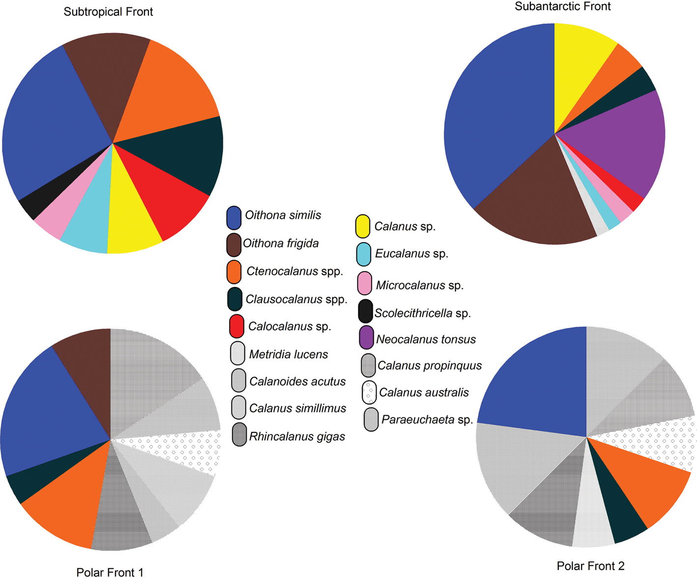
Fig. 4. Relative percentages of copepod species in the surface layer at various frontal regions.
Table V. Variation in surface layer (~2–3 m) dominant copepods presented as average abundance contributions at various frontal regions of the India Ocean sector of the Southern Ocean during summer 2013.

STF = Sub-Tropical Front, SAF = Sub-Antarctic Front, PF = Polar Front.
At the PF1 and PF2, Calanoida and Cyclopoida comprised 52% and 45% of the total zooplankton abundance, respectively, while other taxa occurred in low proportions (appendicularians at 2% and chaetognaths at 1%). The calanoid species that contributed to the total zooplankton abundance were C. acutus, Calanus propinquus, Calanus australis, Calanus simillimus, Rhincalanus gigas, Paraeuchaeta spp., C. citer, Clausocalanus spp. and M. lucens (Fig. 4). Further, O. similis and O. frigida were also important contributors in the PF (Fig. 4).
The surface copepod species diversity ranged from 0.12 to 1.05 and dominance ranged from 0.10 to 0.88 (Fig. 5). The STF had high diversity but low species numbers, while low diversity and species numbers were recorded in the SAF. In contrast, the surface waters between the PF1 and PF2 had high species numbers, with moderately high diversity. No significant differences were observed in diversity among the frontal regions (P = 0.8).

Fig. 5. Spatial variation in zooplankton diversity and dominance (solid line indicates diversity and dashed line indicates dominance).
Zooplankton community structure in the upper 1000 m
When comparing between depth zones, it was clear that the greatest abundance was recorded in the 0–MLD stratum. Diversity increased with depth, while abundance decreased. Vertical distributions of zooplankton communities were broadly associated with various depth layers in the present study. Our results indicate that the high zooplankton abundance in the Indian sector of the SO is mostly concentrated within the MLD during the summer.
Copepods were the numerically dominant group at most stations and in most depth strata. Clausocalanus spp., Ctenocalanus spp., Calocalanus spp., Calanus spp. and Oithona spp. dominated in the upper 150 m at stations STF4 and SAF3 (Table VI). Within the Clausocalanidae, Clausocalanus laticeps was largely responsible for the increased abundance in the upper 150 m. Within the Oithonidae, O. similis was largely responsible for the extremely high abundances between 0 and the MLD. Relatively, much lower numbers of Oithona spp. occurred in the MLD–150 m depth layer. In particular, Calocalanus spp. were common at station STF4, while N. tonsus was abundant at station SAF3 (Table VI). Rhincalanus gigas, Paraeuchaeta spp., Pleuromamma spp., Metridia spp., Calanus spp. and Haloptilus spp. contributed significantly to zooplankton abundance at depths > 150 m. Candacia spp. were restricted to 150–300 m depths, Eucalanus longiceps was found only at station STF4 and Heterorhabdus spp. were found only at station SAF3 between 150 and 1000 m. Furthermore, small ubiquitous copepods in the genus Oncaea were more important at between 150 and 500 m depths at station STF4 and SAF3 (Table VI). Calanus propinquus, C. acutus, Clausocalanus spp., Ctenocalanus spp. and Oithona spp. were major contributors to the total zooplankton abundance at between 0 and 150 m at stations PF1 #2 and PF2 #5 (Table VI). To a greater or lesser extent, within the Oithona spp., O. frigida was largely responsible for the increased abundance in the 0–MLD depth, along with the less abundant O. similis. Calanoides acutus was important at the MLD, while Microcalanus spp. were restricted between the MLD and 150 m, and Candacia spp. were encountered mostly in the 150–300 m stratum. Between 150 and 500 m, Pleuromamma spp., Metridia gerlachei, R. gigas and Paraeuchaeta spp. occurred in large numbers (Table VI). In addition to copepod species, non-copepods were also encountered less frequently. Most of the non-copepod groups, including chaetognaths and appendicularians, were abundant typically in the upper 150 m across most of the sampling locations (Table VI). These two groups were important contributors to the total abundance in the study area. Within the depth range (0–MLD), these two taxa were numerically more dominant at stations PF1 #2 and PF2 #5 than at STF4 and SAF3. In contrast, in the depth range between MLD and 150 m, they were relatively more numerous at stations STF4 and SAF3 (Table VI).
Table VI. Percentage compositions of dominant copepod groups, chaetognaths and appendicularians sampled throughout the water column at four oceanographic stations.

n/a = data not available, MLD = depth of mixed layer, STF = Sub-Tropical Front, SAF = Sub-Antarctic Front, PF = Polar Front.
Discussion
Influence of nutrients on chl a distribution
The low nutrient concentrations observed in the STF and SAF, coupled with low chl a concentrations and low zooplankton biovolume, may be explained by limiting micronutrients (presumably iron) and/or strong zooplankton grazing. It is well documented that iron limits primary production in high-nutrient, low-chlorophyll regions (e.g. Martin & Fitzwater Reference Martin and Fitzwater1990). In the PF, the high sea level pressure gradients and the low temperatures due to the Southern Annular mode define this region as an upwelling area, which brings nutrient-rich waters to the sea surface. The increase in nutrients triggers the high phytoplankton biomass and eventually promotes a high zooplankton biovolume. Furthermore, iron input from sedimentary sources most probably plays an important role in this region (Moore & Abbott Reference Moore and Abbott2002). During the present study, relatively larger phytoplankton cells (diatoms) were found to be dominant at the PF due to the combination of higher silicate and ammonium concentrations than in the STF. Earlier studies reported concentrations of 4 μM in the SO Global Ecosystem Dynamics survey (Serebrennikova & Fanning Reference Serebrennikova and Fanning2004) and 4 μM in the Ross Sea (Gordon et al. Reference Gordon, Codispoti, Jennings, Millero, Morrison and Sweeney2000) in the summer. In the present study, the concentration was 34.45 μM in the Indian sector of the SO (56°30'S). Moore & Abbott (Reference Moore and Abbott2002) stated that mesoscale physical processes, including meander-induced upwelling and increased eddy mixing, where the PF encounters large topographic features, probably lead to increased nutrient flux to surface waters over the Keruguelen Plateau. Previous research by Naik et al. (Reference Naik, Jenson, Melena, Asha, Anilkumar and Rajdeep2015) showed that higher silicate concentrations in the environment favour the growth and development of larger phytoplankton cell such as diatoms. Sommer (Reference Sommer1986) stated that the silicate uptake range is quite high in the PF; therefore, this region is dominated by the bloom forming large-celled or long-chained diatom species (e.g. Fragilariopsis kerguelensis, Corethron criophilum, Thalassiothrix spp.). In this respect, our observations support the notion that the growth condition of the phytoplankton biomass (diatoms) was very favourable as a preferential food source, which strengthens the persistence of larger calanoid copepods and their high abundance in this area. It should also be noted that the species at higher latitudes tend to have larger body sizes. In particular, polar organisms’ body sizes are governed by physical, ecological and evolutionary principles (Moran & Woods Reference Moran and Woods2012). Picophytoplankton dominated at the STF and SAF, where lower silicate and ammonium concentrations were found; the growth rate of phytoplankton cells in this region might be limited by low silicate concentrations (Boyd et al. Reference Boyd, Crossley, DiTullio, Griffiths, Hutchins, Queguiner, Sedwick and Trull2001). Consequently, the size of the copepods was relatively small, as the smaller zooplankton size fractions feed preferentially on picophytoplankton and nanophytoplankton (Froneman & Perissinotto Reference Froneman and Perissinotto1996).
Horizontal distribution of zooplankton communities and species assemblages
In general, the taxa in the surface layer showed broad distributions between fronts. However, they were not vastly different between stations. Most species occurred in adjacent fronts and are considered cosmopolitan, with only few endemic species occurring in particular fronts. The STF community was characterized by low densities of common taxa such as C. citer and Oithona spp. It is possible that low chl a coupled with high temperatures might have led to low zooplankton abundance in the STF. In addition to this, both small copepods O. similis and C. citer probably have reproductive peaks in early spring, and therefore copepodite stages I–III dominate their populations from December to January (Atkinson Reference Atkinson1998). Furthermore, the differences in sampling times will influence growth more than abundance (i.e. development to later stages) (Swadling et al. Reference Swadling, Penot, Vallet, Rouyer, Gasparini and Mousseau2011). Small zooplankton, especially copepods, were probably greatly under-sampled, as previously noted by Hunt & Hosie (Reference Hunt and Hosie2006b). The copepodite stages of O. similis and C. citer might have been missed in the bongo net samples by not being trapped by the 200 μm mesh. Mesozooplankton in the SO are usually sampled with 200 μm mesh nets, although a more suitable size is 100 μm mesh nets, and these will still under-sample juvenile stages of some cyclopoid species (Swadling et al. Reference Swadling, Penot, Vallet, Rouyer, Gasparini and Mousseau2011). Therefore, the abundances of many of the copepod species are probably underestimated. Dominant species/taxa showed similar distribution patterns between the STF and SAF. They are also the same species previously observed in the STF (Takahashi et al. Reference Takahashi, Hosie, McLeod and Kitchener2011). In particular, C. citer is known to be a strong seasonal migrant able to spawn in early spring, even at low chl a concentrations (Atkinson Reference Atkinson1998), while O. similis is known to be adapted to the low phytoplankton densities of the permanent open ocean zone (Takahashi et al. Reference Takahashi, Kawaguchi, Hosie, Toda, Naganobu and Fukuchi2010a). Another explanation for this is that the differences in phytoplankton community structure may also have influenced the zooplankton communities, as the occurrence of smaller picophytoplankton and nanophytoplankton and low autotrophic primary production might indicate a microbial-based food web, in which secondary production is observed in the presence of insufficient autotrophic resources. Several widespread taxa had continuous distributions, being present at the STF and also present in the vicinity of the SAF. Oithona spp., Ctenocalanus spp. and Clausocalanus spp. were all important. Ctenocalanus citer was largely responsible for the increased abundance in the surface layers, which was largely due to the presence of younger stages during the summer months. Compared with the other three copepods, N. tonsus and Calanus spp. were also relatively abundant. A similar SAF community has also been identified in the south Atlantic Ocean and in the Pacific Ocean south of New Zealand (Atkinson & Sinclair Reference Atkinson and Sinclair2000). Neocalanus tonsus was numerically dominant in the SAF, which is characteristic of this copepod (Letterio & Ianora Reference Letterio and Ianora1995).
Generally, the PF has been noted as a region of enhanced phytoplankton and zooplankton abundance in the SO (Atkinson & Sinclair Reference Atkinson and Sinclair2000). In the present study, enhanced chl a was observed in the vicinity of the PF, lending support to the ecological importance of this front. Higher phytoplankton concentrations stimulate grazing, which enhances zooplankton biomass. It is possible that the availability of diatom-dominated phytoplankton biomass in the PF enhanced zooplankton biomass. The usual time lag between phytoplankton blooms and grazer development enabled the high phytoplankton biomass due to high levels of nutrients in the vicinity of the PF. Carlotti et al. (Reference Carlotti, Thibault-Botha, Nowaczyk and Lefevre2008) reported that when the ecosystem structure was dominated by large diatoms, it provided favourable conditions for the large copepods in the Kerguelen Plateau area. This supports our observations that the PF was dominated by larger species, such as C. propinquus, C. acutus, C. australis, C. simillimus and R. gigas. Increased copepod abundance in response to high phytoplankton biomass has previously been observed at South Georgia Island (Atkinson et al. Reference Atkinson, Shreeve, Pakhomov, Priddle, Blight and Ward1996), where copepod life cycles involve reproduction and early larval feeding in summer, with later lipid-rich stages being less active, spending the winter in diapauses or least with reduced activity, and often at depth (Atkinson Reference Atkinson1998, Pakhomov et al. Reference Pakhomov, Froneman and Perissinotto2002). Higher population densities of small copepods were also observed, mainly comprising O. similis and C. citer, apparently contributing significantly to food web dynamics as in the PF. In particular, high chl a concentrations in the surface layer may have been the driving force behind the tendency of copepod species to concentrate closer to the surface. If our assumption holds true, these copepods are key elements in the transfer of organic matter to the higher trophic food levels in the open Antarctic Ocean. The small copepods, such as O. similis and C. citer, have been recognized to be both highly abundant and important in energy flow (Atkinson Reference Atkinson1998). In the current study, there was considerable temporal variation in the mean abundance of the zooplankton assemblages between the months, ranging from 550 ind m−3 in late January 2013 to 12 452 ind m−3 in late February 2013. Our finding also shows that during the summer, large changes in surface zooplankton community structure were observed, and the average transect abundance of smaller copepods peaked abruptly in early February and then remained high. The high abundance recorded in February may have reflected the overwintering and/or adult reproductive population. Undoubtedly, monthly variations in this survey may also have influenced our observations of zooplankton distributions. Among the mesozooplankton, chaetognaths and appendicularians were often second only to copepods in abundance and biomass, and their population density was low due to their ability to adapt to the prevailing environmental conditions. The predominant taxa were Mesosagitta spp., Sagitta spp., Oikopleura spp. and Fritillaria spp. Similar results have been observed near the coastal area east of the Kerguelen Islands in the Indian sector of the SO (Carlotti et al. Reference Carlotti, Jouandet, Nowaczyk, Harmelin-Vivien, Lefèvre and Richard2015).
Vertical distribution of the zooplankton community dynamics
Zooplankton biomass, abundance and community structure were strongly structured in the vertical plane, and the distributions of a number of species varied between depth zones. The relationship between MLD and zooplankton biomass is complex. For example, deepening of MLD influences the availability of light and nutrient supply, which would determine phytoplankton growth and subsequently cause changes in zooplankton biovolume and community structure; hence, zooplankton biovolume increased with deeper MLD. The zooplankton biovolume and community structure in the Indian sector of the SO would therefore be expected to respond to changes in the mixed layer. Copepods were the greatest contributor to total species abundance in all depth zones. In particular, we observed distinct communities between stations STF4 and SAF3. The numerical dominance of small copepods, such as Clausocalanus spp., Ctenocalanus spp. and Oithona spp., in the upper and mesopelagic zones is similar to that previously reported in the SO (Hunt & Hosie Reference Hunt and Hosie2006a). Oithona similis was the most numerically abundant copepod (Hunt & Hosie Reference Hunt and Hosie2006a) and is considered to be a key component of the plankton food web of the SO (Atkinson Reference Atkinson1998), forming a significant proportion of the zooplankton biomass despite its small size. Clausocalanus spp., Ctenocalanus spp. and Oithona spp. were more numerous in the MLD than the lower layer (MLD–150 m); this small peak in the MLD–150 m layer could be due to the downwards migration of pelagic species in order to avoid predation. South of the PF (stations PF2 and PF5), species such as C. propinquus and C. acutus inhabited the low-temperature waters and were distributed widely within the PF. The present study showed that the vertical distributions of zooplankton communities were broadly associated with various depth layers. Copepods were strongly structured in the vertical plane, and the distribution of the number of species varied between depth zones. This was reflected by increased species diversity and decreased dominance with depth. This is probably to be due to smaller gradients in oceanographic properties in the deeper layer compared to those in the epipelagic layer. The depth distribution of Paraeuchaeta spp., R. gigas, Metridia spp. and Pleuromamma spp. showed that they were most abundant in the 150–1000 m layer, but this does not account for the disparity in abundance levels. Representatives of various genera that co-occurred in the same depth range generally differed in feeding behaviour and dietary preferences, as evidenced by trophic biomarkers (Laakmann et al. Reference Laakmann, Stumpp and Auel2009). In fact, most calanoid species in the SO are found in deep waters (mesopelagic and bathypelagic layers) (Ward & Shreeve Reference Ward and Shreeve2001). This indicates that vertical differences in environmental factors are important for determining copepod community structure. In addition to copepods, appendicularians and chaetognaths were relatively important zooplankton contributors to the total zooplankton biomass. Appendicularians are filter-feeders, while chaetognaths are voracious predators of copepods and are generally found at depths coinciding with copepod vertical distribution. Appendicularians are one of the common members of zooplankton communities in all oceans, and they are ideally suited to oceanic oligotrophic conditions (Deibel Reference Deibel and Bone1998).
Influence of temperature on variation in the size fraction of common copepod taxa
Size fractionation of the copepod community provides information on what size classes primarily contribute to the various frontal regions. Copepod size is particularly important because it can be an indicator of multiple biological and ecological traits, such as metabolism, feeding strategy (Kiørboe Reference Kiørboe2011) and tropic links. The present data reveal that larger copepod species (> 2 mm) dominated in cooler regions where temperatures were < 4°C and smaller species (< 2 mm) were dominant in warmer regions where temperatures were > 18°C; thus, it appears that warmer conditions favour the dominance of smaller species (Daufresne et al. Reference Daufresne, Lengfellner and Sommer2009). This finding demonstrated that the discrepancy in the interspecific temperature–size relationship could be explained by a geographical shift of the thermal niche boundary of these species. We observed a positive relationship between copepod size and water temperature in the SO, with the result being that larger copepods were more dominant in the cooler waters than warmer waters. The copepod size structure may change further with advection transport and latitudinal shift in water masses, which are driven by oceanic current dynamics. Clausocalanus spp., Ctenocalanus spp., Calocalanus spp., Microcalanus spp., Scolecithricella spp. and Oithona spp. were the major contributors to the < 2 mm group, similarly to an earlier report (Koubbi et al. Reference Koubbi, Hulley, Raymond, Penot, Gasparini and Labat2011). On the other hand, C. propinquus, C. australis, C. simillimus, C. acutus, N. tonsus, E. longiceps, Paraeuchaeta spp, and R. gigas were the major contributors to the > 2 mm group. The Kerguelen Plateau was characterized by a greater abundance of large calanoid copepods such as R. gigas and Paraeuchaeta spp. (Carlotti et al. Reference Carlotti, Jouandet, Nowaczyk, Harmelin-Vivien, Lefèvre and Richard2015). The success of the numerically dominant species R. gigas and Paraeuchaeta spp. was probably due to their different life stages (Atkinson Reference Atkinson1998). Compared to larger copepod species, smaller warm-water species dominated the surface region of the study area. This pattern was the opposite of the vertical distribution of copepod species. Larger copepod species at station STF4 mostly resided at < 500 m where the temperature was < 4°C; correspondingly, they were present at < 300 m in station SAF3, where the temperature was < 4°C, indicating that a particular temperature was probably serving as the boundary of the thermal niche for the larger copepod species. A question arises as to why the larger fraction of zooplankton occurred at discrete depths. One of the major factors determining the distribution of larger individuals is that they experience greater susceptibility to visual predators, and hence they have a need to descend below the euphotic depth during the day, moving to the surface layers soon after sunset. This behaviour in the large-sized copepods may have caused the strong day/night difference in their distribution pattern. The results of this study demonstrate that water temperature is probably more important than phytoplankton food availability in determining the distribution limit of these species.
Summary and conclusion
The community structure of zooplankton reflected their sensitivity to their surroundings and highlighted their dominance in various frontal regions. Nutrient concentrations were lower in the STF than the PF regions, which led to higher chl a concentrations in the latter, corresponding with greater zooplankton abundance. The supply of micronutrients and grazing pressure by zooplankton controlled the onset and duration of the phytoplankton growth period. Lower chl a was observed at the SAF and STF, coinciding with low nutrient concentrations and indicating that control of autotrophic production was mainly dependent on the presence of high levels of nutrients. The highest silicate concentrations were observed in the PF, suggesting the dominance of diatoms and indicating spatial coupling between primary and heterotrophic production in the PF. Chl a played a major role in driving the spatial distribution of zooplankton biomass. Similarly to other oceans, copepods numerically dominated the total mesozooplankton in the study region. Calanoida was the dominant zooplankton group in the PF1 region and Cyclopoida was the dominant zooplankton group in the PF2 region. The ecological differences in these communities therefore reflected the physical heterogeneity of the region between the STF, SAF and PF. Ctenocalanus citer, C. laticeps and O. similis were the dominant species during the study period. The taxonomic composition did not show major differences between stations near each front. We found an increase in copepod community size from the STF to the PF because of the increased dominance of large cold-water species due to decreases in temperature. Therefore, environmentally forced changes in the zooplankton community structure may have important implications for ecosystem functioning.
Acknowledgements
We express our sincere gratitude to the Director of the National Centre for Polar and Ocean Research for facilities and encouragement. We thank the Director of the National Institute of Ocean Technology (NIOT) and the Head of the Vessel Management Cell (VMC) for providing us the platform and other essential logistical support. We sincerely acknowledge the captain, officers and crew members of the seventh Indian scientific expedition to the Southern Ocean. We thank the two reviewers for their helpful comments on the manuscript. The NCPOR contribution number is J-50/2019-20.
Author contributions
VV, SCT and NA conceived and designed the study. VV wrote the manuscript, and the final manuscript was improved by KS. Fieldwork and analysis were performed by VV, RKM, AS, SMA, PS, SCT and HUKP. All authors agreed to submit it to Antarctic Science.
Supplemental material
Two supplemental tables will be found at https://doi.org/10.1017/S0954102019000579.


