Introduction
As a transitional zone from land to sea, Antarctic coastal waters are among the most unstable marine habitats for living organisms. Nearshore conditions appear to be conducive to producing massive phytoplankton blooms in summer (Smith et al. Reference Smith, Baker and Vernet1998). At that time, the variations of phytoplankton biomass and communities serve as important and sensitive indicators of environmental perturbations (Ahn et al. Reference Ahn, Chung, Kang and Kang1997). Meanwhile, the overall change of phytoplankton productivity is, in turn, likely to impact the structure and function of coastal food webs (Moline et al. Reference Moline, Claustre, Frazer, Schofield and Vernet2004).
Several environmental factors influence phytoplankton growth in summer. Temperature and salinity change as sea ice melts, which promote well stratified surface waters and allows some ice species to flourish (Smith et al. Reference Smith, Baker and Vernet1998, Lange et al. Reference Lange, Tenenbaum, De Santis Braga and Campos2007, Annett et al. Reference Annett, Carson, Croata, Clarke and Ganeshram2010). Nutrient variations (due to additional terrestrial inputs), light limitation (due to high turbidity) and the strong mixing (a consequence of the heavy winds) have also been suggested to control phytoplankton blooms (Schloss et al. Reference Schloss, Ferreyra and Diana2002).The wind-driven re-suspension of benthic forms and influence of open water species on the phytoplankton community of Antarctic coastal waters both need to be considered (Ahn et al. Reference Ahn, Chung, Kang and Kang1997, Piquet et al. Reference Piquet, Bolhuis, Meredith and Buma2011). Moreover, the western Antarctic Peninsula (WAP) has been established as one of most rapidly warming regions (Hansen et al. Reference Hansen, Ruedy, Glascoe and Sato1999, Vaughan et al. Reference Vaughan, Marshall, Connolley, Parkinson, Mulvaney, Hodgson, King, Pudsey and Turner2003, Meredith & King Reference Meredith and King2005, Stammerjohn et al. Reference Stammerjohn, Martinson, Smith and Iannuzzi2008) which results in decreased duration of sea-ice cover, increased glacial meltwater runoff and reduced surface water salinities (Meredith & King Reference Meredith and King2005, Stammerjohn et al. Reference Stammerjohn, Martinson, Smith and Iannuzzi2008). All these changes would significantly influence the community structure and stocks of phytoplankton and even food webs in coastal Antarctic waters (Clarke et al. Reference Clarke, Murphy, Meredith, King, Peck, Barnes and Smith2007, Annett et al. Reference Annett, Carson, Croata, Clarke and Ganeshram2010, Piquet et al. Reference Piquet, Bolhuis, Meredith and Buma2011).
Some studies focusing on Antarctic coastal phytoplankton blooms have been reported (Ahn et al. Reference Ahn, Chung, Kang and Kang1997, Smith et al. Reference Smith, Baker and Vernet1998, Clarke et al. Reference Clarke, Meredith, Wallance, Brandon and Thomas2008, Piquet et al. Reference Piquet, Bolhuis, Meredith and Buma2011), but those were based on the method of a certain sampling frequency (one to several times per month). Here we deployed an online mooring system in Great Wall Bay (unofficial name) to monitor the environmental variation and phytoplankton blooms in Antarctic coastal waters. Such a system is commonly used in marine sites at lower latitudes (e.g. Lips et al. Reference Lips, Lips, Liblik, Kikas, Altoja, Buhhalko and Ruenk2011, Strutton et al. Reference Strutton, Martz, Degrandpre, McGillis, Drennan and Boss2011). However, in Antarctica only a few studies have deployed moorings in coastal waters (Fukuchi et al. Reference Fukuchi, Hattori, Sasaki and Hoshiai1988, Smith et al. Reference Smith, Asper, Tozzi, Liu and Stammerjohn2011).
The Great Wall Bay is located in King George Island, South Shetland Islands, where meteorological monitoring at the Great Wall Station from 1985–2008 has shown air temperatures to be increasing at a rate of 0.27°C per decade (Bian et al. Reference Bian, Ma, Lu and Lu2010). Using the mooring system, a range of environmental variables (temperature, salinity, depth, pH, photosynthetically active radiation (PAR) and chlorophyll a (chl a) concentration in the water column) were recorded in summer (between 13 December 2010 and 23 March 2011), allowing the phytoplankton blooms and their possible drivers to be analysed, and the reliability of the mooring system to be evaluated.
Methods and site
Figure 1 shows the locations of the site and Fig. 2 shows a schematic diagram of the online coastal mooring system. The system was deployed in the deepest area in the Great Wall Bay in 2010. The bay has a maximum depth of c. 35 m near the top of the bay, and the site was c. 200 m from the coast and c. 30 m underwater. The floats were placed about 5 m beneath the surface to avoid damage from ice. Electricity was supplied from the Great Wall Station and environmental parameters - temperature, salinity, depth, pH, PAR, chlorophyll (at 2–3 depths), and water current in the water column - were monitored with in situ CTD (conductivity, temperature, depth) and ADCP (Acoustic Doppler Current Profilers). Data were recorded every ten minutes and transferred to the station computer through a cable. Two SBE 16 CTDs were fixed on the mooring wire, and one SBE37 CTD and one TRDI Workhorse 600 kHz ADCP were fixed on the bottom platform. Sensors were fixed at 12.9 m, 19.6 m and 29.7 m depths respectively. These sensors are referred to as the upper, middle and bottom layers.
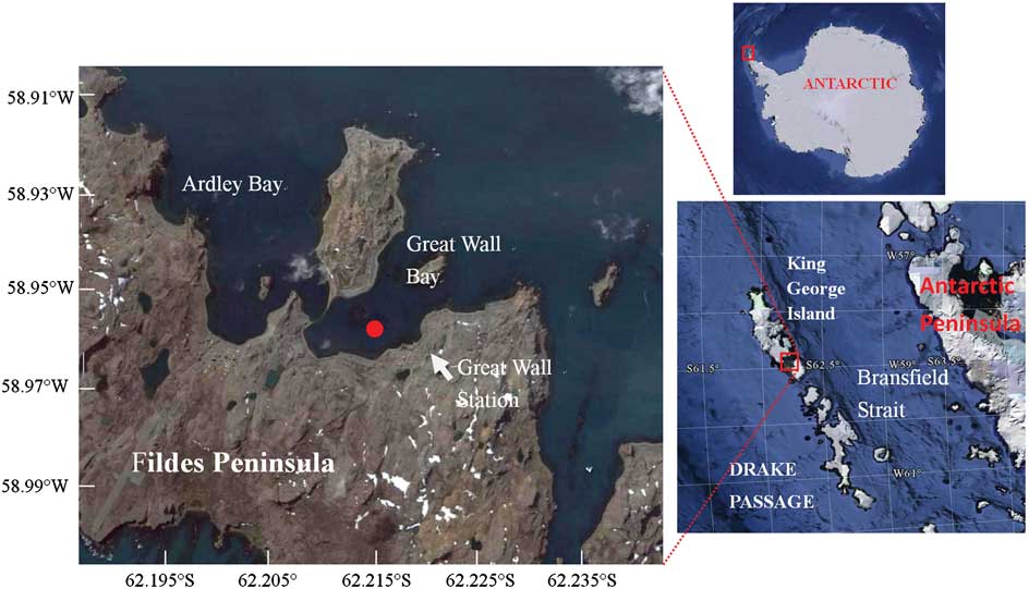
Fig. 1 Locations of the mooring site in the Great Wall Bay, King George Island, Antarctica. The map is taken from Google Earth, accessed November 2011.
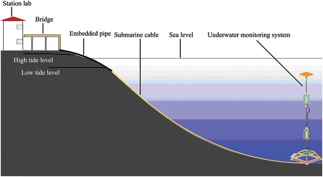
Fig. 2 Schematic diagram of the coastal mooring system.
Data for temperatures, salinities and chl a concentrations were averaged daily to detect trends. The entire monitoring period was divided into several sub-periods determined by the variations of chl a and a piecewise analysis was conducted to explore the potential reasons for the fluctuation of phytoplankton biomass. Pearson correlation and partial least squares (PLS) analysis were used. The coefficients for standardized environmental factors (zT, zS, zD, zpH and zPAR) were calculated and regression equations were also fitted. All of the statistical analyses were done by the software SPSS 17.0.
Results
Distribution and variation of environmental variables
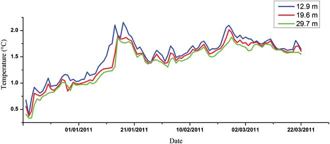
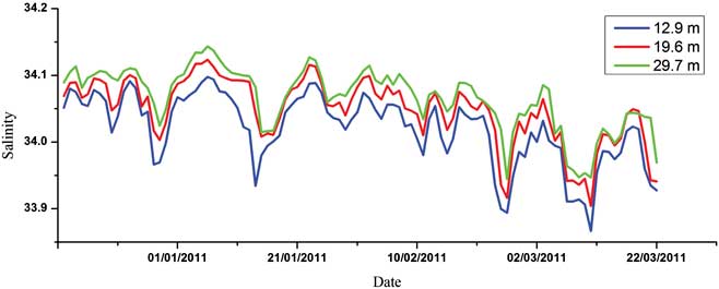
Figures 3–5 show the variations of temperature, salinity and chl a concentration, respectively. In general, temperature decreased from upper to lower levels and showed an increasing general trend during the monitoring period (0.27–2.52°C). Obvious peaks were observed in mid-January and late February and significant linear correlations were discovered between different water layers (r 2 = 0.919, 0.873 and 0.969 for upper/middle, upper/bottom and middle/bottom layers respectively). In contrast to temperature, salinity increased from upper to lower levels and showed a decreasing trend during the observation period (34.19–33.86). Obvious linear relationships were also revealed between different layers (r 2 = 0.793, 0.640 and 0.737 for upper/middle, upper/bottom and middle/bottom layers respectively). Temperature and salinity showed a linear correlation in the upper layer (r 2 = 0.488), but no relationship was observed for the middle or bottom layers. We conclude that the influence of freshwater input was more significant for the upper layer. The temperature and salinity data at no point suggested that the water column was totally mixed, and the upper layer waters showed evident stratification with both the middle and bottom layers throughout the time series. Moreover, PAR signals also displayed significant variations through the whole monitoring exercise with two extremely low periods in January and March, respectively. It also showed characteristics of diurnal cycles with troughs at early hours in the morning and peaks at noon (Fig. 6).

Fig. 3 Seasonal variation of water temperature in the Great Wall Bay (daily average).
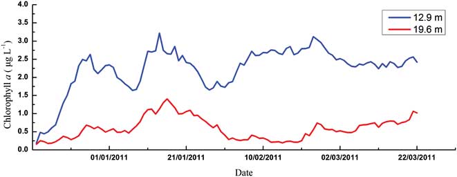
Chlorophyll a concentration, considered as an indicator of the phytoplankton biomass, showed strong seasonal variability and an increasing trend in both upper and middle layers during the monitoring period (Fig. 5). In the upper layer, biomass accumulated from mid-December and two strong blooms developed through January (3.18 μg l-1 and 4.75 μg l-1, respectively), and then were maintained at a relatively high level, with a transient bloom in late February (4.93 μg l-1). In the middle layer, chl a concentrations were much lower compared with those in the upper layer. Despite an obvious peak in mid-January (2.45 μg l-1), the phytoplankton blooms in late December and late February were not evident (1.05 μg l-1 and 1.98 μg l-1).
Correlations between chl a, temperature and salinity
The monitoring period was sub-divided into several time intervals to further investigate the contribution of different environmental variables to the variation in phytoplankton biomass (Tables I & II). The results of Pearson correlation analysis showed the significant and positive influence of temperature variation on phytoplankton biomass fluctuation, especially during phytoplankton blooms, whereas the salinity showed significant and negative correlations with chl a during phytoplankton blooms (Tables I & II). According to the results of PLS analysis (Tables III & IV), temperature had a greater effect on phytoplankton biomass variation than salinity. The significant and negative relations between temperature and salinity might contribute to the significant and negative relations between salinity and chl a in Pearson correlation analysis.
Table I Correlation analysis between chlorophyll a (chl a) concentrations and environmental variables for upper level during different timescales. Time periods are expressed as day.month.
*Correlation is significant at the 0.05 level (2-tailed).
**Correlation is significant at the 0.01 level (2-tailed).
Table II Correlation analysis between chlorophyll a (chl a) concentrations and environmental variables for middle level during different timescales. Time periods are expressed as day.month.
*Correlation is significant at the 0.05 level (2-tailed).
**Correlation is significant at the 0.01 level (2-tailed).
Table III The fitted regression equation of chlorophyll a (chl a) concentrations with environmental variables by partial least squares analysis. Time periods are expressed as day.month.
Table IV The standardized coefficient of partial least squares analysis.

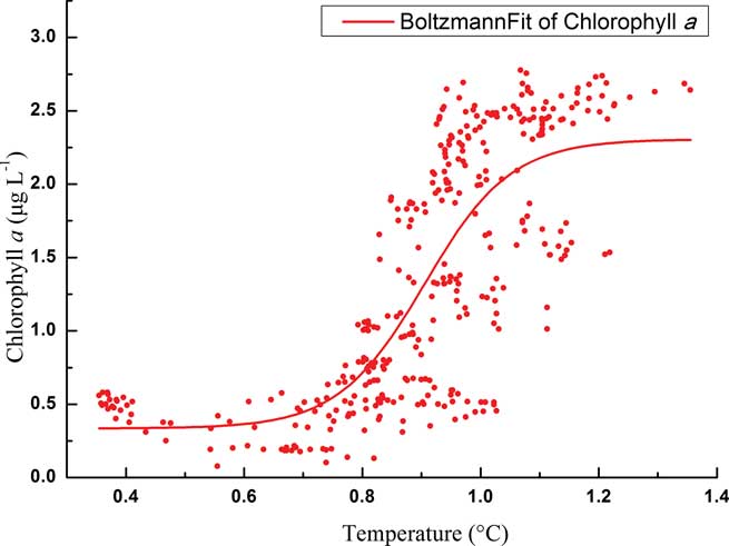
Total phytoplankton biomass in the upper layer displayed a typical growth pattern of two chl a peaks from December–January (Fig. 5), but their links with temperature showed quite distinctive patterns. For the initial bloom, the variation of phytoplankton biomass showed an “S-shape” curve with temperature according to a Boltzmann fit (Fig. 7). Specifically, phytoplankton biomass was limited to < 0.5 μg l-1 at the beginning of the monitoring with relatively lower temperatures (c. 0.35°C–0.75°C). 0.8°C seems to be a threshold for the initial phytoplankton bloom. As the temperature increased up to 1°C, chl a concentration also increased dramatically to about 2.5 μg l-1. After that, phytoplankton biomass maintained a plateau at around 2.5 μg l-1. However, for the second chlorophyll peak, there were no chl a plateau periods during the bloom, and phytoplankton biomass increased dramatically from 1.5–3.5 μg l-1 as temperatures increased from 1.2–2.2°C.

Fig. 7 Boltzmann fit of chlorophyll a in relation to temperature during the initial bloom in the upper level.
Relationships between PAR and chl a
Photosynthetically active radiation was also an important environmental factor affecting phytoplankton growth. It was noted that the retreat of the second phytoplankton bloom corresponded to the extremely low levels of PAR in January. Meanwhile, as shown in the Pearson correlation and PLS analysis results, the correlations between PAR and chl a converted from negative relations during the bloom period to the positive ones during the stable period for the upper layer (Table I), which suggested their physiological light-adaptation process from spring to summer. However, continuously negative correlations were discovered for the phytoplankton of the middle layer (Table II). As PAR levels decreased significantly from the upper layer to the middle layer (Fig. 6), light-adaptive characteristics of phytoplankton at the relatively deeper layers might be shade-adapted. To further clarify reasons inducing PAR attenuation between upper and middle layers, we calculated the attenuation of PAR and compared the changes of this attenuation to the changes in chlorophyll and PAR level itself. The attenuation showed significant and negative correlations with both chl a concentrations at 13 m and 20 m (R13m-chl a = -0.614, R20m-chl a = -0.563, P < 0.01, n = 100). The attenuation was quite high when the PAR level at 13 m and 20 m were high (R13m-PAR = 0.990, R20m-PAR = 0.938, P < 0.01, n = 100). The attenuation might be attributed to particulates originating from land and wind-induced turbulence rather than phytoplankton.
Discussion
Occurrence of phytoplankton blooms in Antarctic coastal waters
It is suggested that massive blooms in summer are a significant component of the shelf ecosystem in the Antarctic (Ahn et al. Reference Ahn, Chung, Kang and Kang1997, Smith et al. Reference Smith, Baker and Vernet1998). Our online mooring system suggested that biomass accumulated from mid-December; two obvious blooms developed through January and were then maintained at a relatively high level, with a transient bloom in late February, which is comparable to the conditions in other Antarctic coastal waters. A four-year time series (1991–95) sampling in the vicinity of Palmer Station suggested that generally two blooms occurred, a relatively large spring bloom during December/January and a smaller secondary bloom in February/March and blooms appeared to be more persistent in years of higher chl a accumulation, with additional peaks between the two typical bloom periods (Smith et al. Reference Smith, Baker and Vernet1998). Chlorophyll a in Ryder Bay near Rothera Station also often showed two distinct peaks during the growing season (Clarke et al. Reference Clarke, Meredith, Wallance, Brandon and Thomas2008). Moreover, our monitoring of phytoplankton biomass is generally comparable to the historical records for Great Wall Bay (Table V). When compared to other Antarctic nearshore waters, our results are a little lower than Ryder Bay and coastal waters of Palmer Station, but similar to Maxwell Bay and Admiralty Bay, which are close to our site (Table V).
Table V Comparison of chlorophyll a with historical records of Great Wall Bay and other Antarctic coastal waters. Periods are shown as month.year.
*Average value
Regulation of chl a with temperature and salinity
Temperature plays an important role influencing phytoplankton biomass in our study. The importance of temperature has been demonstrated by several laboratory experiments (Reay et al. Reference Reay, Priddle, Nedwell, Whitehouse, Ellis-Evans, Deubert and Connelly2001) and field monitoring (Lange et al. Reference Lange, Tenenbaum, De Santis Braga and Campos2007, Annett et al. Reference Annett, Carson, Croata, Clarke and Ganeshram2010), but only the online mooring system could detect small-scale variations. Generally, the terrestrial freshwater and/or sea-ice meltwater were the main runoff sources in the Antarctic coastal areas in early summer. The sea-ice meltwater had low temperature and salinity, whilst terrestrial freshwater was warmer and although of low salinity contained some additional nutrients (Clarke et al. Reference Clarke, Meredith, Wallance, Brandon and Thomas2008). In our study the first phytoplankton bloom occurred with gradually and slowly increasing temperature and periodically decreasing salinity, which indicated the inputs of moderate temperature, low salinity waters. Thus the sources of freshwater might be the mixture of terrestrial freshwater and sea-ice meltwater with sea-ice meltwater dominating. Such an input would introduce some nutrients and stratify surface waters. Meanwhile, algae freed from melting sea ice will potentially seed the water column (Lizotte Reference Lizotte2001). Previous studies also demonstrated the significant role sea ice played in determining the abundance and distribution of phytoplankton biomass, such as near Anvers Island (Smith et al. Reference Smith, Baker and Vernet1998) and Ryder Bay (Annett et al. Reference Annett, Carson, Croata, Clarke and Ganeshram2010). The flora in Maxwell Bay and Admiralty Bay were both heavily influenced by ice diatoms in early summer (Ahn et al. Reference Ahn, Chung, Kang and Kang1997, Lange et al. Reference Lange, Tenenbaum, De Santis Braga and Campos2007). The plateau period of the “S-shape” curve (Fig. 7) might indicate the time needed by these algae to adapt to the new environment. The “S-shape” curve also revealed minor variations of phytoplankton biomass with temperature due to our continuous monitoring data. The phytoplankton biomass remained stable but grew rapidly when the temperature increased above c. 0.8°C. Therefore, the temperature of c. 0.8°C might be seen as the threshold value for a phytoplanktons bloom in Great Wall Bay. Runoff from the land will bring in nutrients from the excretion of seabirds, seals and penguins (Li Reference Li2004). Thus the time of temperature increase could be seen as the determining factor for the phytoplankton bloom.
For the second phytoplankton bloom, the increase of temperature was continuous and rapid, and the decrease of salinity was more obvious (Figs 3–5). These were indicators for the input of high temperature and low salinity water; thus here the terrestrial input is the dominant freshwater source. With these two blooms, a shift of phytoplankton from cold-adapted species to eurythermal ones might be occurring as was previously observed (Yu et al. Reference Yu, Li and Huang1992).
Both temperature and salinity signals of the upper layer showed evident stratification with both middle and bottom layers (Figs 3 & 4). Although the Antarctic coastal regions are known for strong winds (Schloss et al. Reference Schloss, Ferreyra and Diana2002), the temperature and salinity data suggested at no point was the water column totally mixed. However, both fluctuated greatly indicating lateral intrusion of water with variable levels of salinity and temperature. In addition to sea-ice meltwater and terrestrial freshwater, which enter in early summer, the role of oceanic water advection may not be negligible. In summer, the site exchanges with adjacent oceanic waters from the Bransfield Strait (Chang et al. Reference Chang, Jun, Park and Eo1990). The direct inflows of Antarctic Circumpolar Current from the Bellingshausen Sea and outflows from the Weddell Sea are major sources of water in Bransfield Strait (Hewes et al. Reference Hewes, Reiss and Holm-Hansen2009). Meanwhile, such an intrusion of water would bring in varied phytoplankton species and concentrations as well. That induced a fluctuation of chl a concentration, displaying the distinctive photo-adapted response to PAR. The influence of oceanic waters on the structure of phytoplankton in nearshore waters has been reported both for Maxwell Bay and Admiralty Bay (Ahn et al. Reference Ahn, Chung, Kang and Kang1997, Lange et al. Reference Lange, Tenenbaum, De Santis Braga and Campos2007). In Admiralty Bay the highest abundances were caused by pennate benthic diatoms in early summer, associated with the presence of ice, while centric diatoms were more abundant in late summer, suggesting an influence of oceanic waters (Lange et al. Reference Lange, Tenenbaum, De Santis Braga and Campos2007).

Fig. 4 Seasonal variation of sea water salinities in the Great Wall Bay (with the data of daily average).

Fig. 5 Seasonal variation of chlorophyll a concentrations in the Great Wall Bay (with the data of daily average).
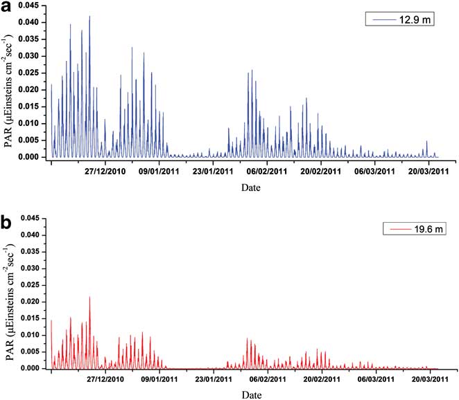
Fig. 6 Seasonal variation of PAR in a. the upper, and b. the middle layer of the Great Wall Bay.
Adaptation of phytoplankton to PAR
Polar primary producers are light limited during the long, near-aphotic winter period, which is exacerbated by the seasonal ice cover (Clarke et al. Reference Clarke, Holmes and White1988, Thomas & Dieckmann Reference Thomas and Dieckmann2002). In early summer, ice meltwater input and terrestrial runoff contains large amounts of organic and inorganic particles, which generates substantial turbidity in the water column (Schloss et al. Reference Schloss, Ferreyra and Diana2002). Although we do not have the PAR data from a station onshore or nearer the surface to evaluate the reduction in PAR with depth due to turbidity, the relationship between temperature and salinity showed negative linear correlations in the upper layer, indicating that the influence of runoff from land was significant. The negative correlations between PAR and chl a at the time of phytoplankton bloom in early summer indicated phytoplankton themselves reduced light transmittance, but on the other hand, it revealed the photo-inhibition or physiological adaptation of phytoplankton to light from the dark period. The turbidity in the water column had a photo-protective effect on phytoplankton growth, especially during the bloom. In early summer phytoplankton at our site might still maintain a relatively shade-adapted characteristic. Photo-inhibition of shade-adapted phytoplankton when they are exposed to strong light, or a reduction of chlorophyll under strong light, have been reported (Morgan-Kiss et al. Reference Morgan-Kiss, Priscu, Pocock, Gudynaite-Savitch and Huncr2006). On timescales of minutes to hours, phytoplankton adaptation is achieved by down regulation of photosynthesis (Lizotte & Sullivan Reference Lizotte and Sullivan1991). On longer timescales of hours to days, it is achieved by adjusting the amount of chl a in each cell, increasing the concentration with a decreasing irradiance and decreasing the concentration with increasing irradiance (Prezelin & Matlick Reference Prezelin and Matlick1980), which have both been demonstrated experimentally (Lizotte & Sullivan Reference Lizotte and Sullivan1991). However, after the bloom the correlations between PAR and chl a changed to positive during the relative stable period. That suggested the gradual physiological light-adaptation process from spring to summer. On the other hand, a shift of phytoplankton from cold-adapted species to eurythermal forms was further confirmed. Some effects of an exchange with oceanic waters from the Bransfield Strait might also contribute to this phenomenon.
Conclusion
Our coastal mooring system captures the overall characteristics and seasonal variation of the nearshore water environment. The basic environmental parameters collected are comparable to the historical records for the region. We conclude that sea-ice meltwater and terrestrial freshwater input caused by the increase of temperature in spring and played an important role in inducing phytoplankton blooms in early summer. The variations of temperature and salinity of different water layers without total mixing suggested lateral intrusion of oceanic waters. The chl a concentrations initially decreased with an increase in irradiance indicating the shade-adapted characteristic of phytoplankton in early summer, followed by a gradual adaptation to increasing irradiance. Our results demonstrate the effectiveness and reliability of the mooring system on the monitoring of environmental variables and phytoplankton blooms in Antarctic coastal waters.
Acknowledgements
We thank the members of all the expeditions who helped to deploy the monitoring system in Antarctica's Great Wall Bay. This work was supported by the National High Technology Research and Development Programme of China (Program 863, No. 2007AA09Z121), the National Ocean Public Benefit Research Foundation (No. 200805095) and the National Nature Science Foundation of China (No. 41076130). The constructive comments of the reviewers are gratefully acknowledged.