


Introduction
In ice-free terrestrial systems of Antarctica, microorganisms are thought to be sentinel organisms: organisms that rapidly respond to climate-driven changes in water, nutrient or sunlight availability in this oligotrophic cold desert environment (Stanish et al. Reference Stanish, Kohler, Esposito, Simmons, Nielsen and Wall2012, Tiao et al. Reference Tiao, Lee, McDonald, Cowan and Cary2012, Lee et al. Reference Lee, Caruso, Archer, Gillman, Lau and Cary2018, Niederberger et al. Reference Niederberger, Bottos, Sohm, Gunderson, Parker and Coyne2019). Strong climate–organism connections are inferred because the physical characteristics of stream habitats are thought to determine the occurrence of the different microbial mats to a greater extent than differences in water quality (McKnight et al. Reference McKnight, Alger, Tate, Shupe and Spaulding2013). A strong relationship between species presence and activity in microbial mats would be consistent with similar relationships observed between mosses in the circum-Antarctic. For example, in the Windmill Islands, Lucieer et al. (Reference Lucieer, Turner, King and Robinson2014) showed that the upstream area could serve as a proxy for water availability from snowmelt, which in turn drove spatial patterns of moss activity.
Cyanobacteria-dominated microbial mats are widely considered as a critical source of organic matter in the otherwise ultra-oligotrophic ecosystem of the McMurdo Dry Valleys (MDVs) (Fritsen et al. Reference Fritsen, Grue and Priscu2000, Moorhead et al. Reference Moorhead, Barrett, Virginia, Wall and Porazinska2003, Hopkins et al. Reference Hopkins, Sparrow, Novis, Gregorich, Elberling and Greenfield2006). However, there is currently no consensus concerning the drivers of the geographical distribution and extent of Antarctic cyanobacteria (Taton et al. Reference Taton, Grubisic, Brambilla, de Wit and Wilmotte2003). Microbial mat heterogeneity is high, even over lengths scales of 1 m or less (Jungblut et al. Reference Jungblut, Hawes, Mountfort, Hitzfield, Dietrich and Burns2005, Karr et al. Reference Karr, Sattley, Rice, Jung, Madigan and Achenbach2005, Zeglin et al. Reference Zeglin, Sinsabaugh, Barrett, Gooseff and Takacs-Vesbach2009). If different mat types (determined by the identity of characteristic cyanobacteria) respond rapidly and in environmentally diagnostic ways to changing physical conditions, then there is a need to be able to monitor the extent and activity of Antarctic microbial mats as a system proxy that would be useful for detecting regional changes in runoff and biogeochemistry in an environment that is on the brink of major climatic and hydrological change (Fountain et al. Reference Fountain, Levy, Gooseff and van Horn2014, Levy et al. Reference Levy, Fountain, Obryk, Telling, Glennie and Pettersson2018). Critically, microbial mats in MDV streams respond rapidly, over days to weeks, to changes in water availability (McKnight et al. Reference McKnight, Niyogi, Alger, Bomblies, Conovitz and Tate1999). Changes in metabolic activity from dormant to active and growing are expressed via changes in pigmentation intensity and visibility, transitioning from ‘cryptic’ and indistinguishable from background red-grey sediments to orange and black colours apparent upon inspection (McKnight et al. Reference McKnight, Niyogi, Alger, Bomblies, Conovitz and Tate1999).
Based on research in warm desert environments, we suggest that hyperspectral reflectance remote sensing may serve as a sensitive tool for mapping the spatial extent and species characteristics of cold desert microbial mats in Antarctic cold deserts. For example, Schmidt & Karnieli (Reference Schmidt and Karnieli2000) used satellite hyperspectral observations of vegetation in the semi-arid Negev Desert to distinguish biogenic crusts from sands and regolith, even when during the dry season sands and biogenic crusts were nearly indistinguishable by visual inspection.
In Antarctica, biological communities typically have an extremely small spatial footprint, forming in patches at the metre to decametre scale. In order to capture these small biological communities, high-spatial-resolution imaging and reflectance remote sensing have been carried out in order to study these limited biotic exposures using low-altitude unmanned aerial systems (UASs), also known as remotely piloted aircraft systems (RPASs), unmanned aerial vehicles (UAVs) or drones (Lucieer et al. Reference Lucieer, Turner, King and Robinson2014, Malenovsky et al. Reference Malenovský, Turnbull, Lucieer and Robinson2015, Reference Malenovský, Lucieer, King, Turnbull and Robinson2017). Prior studies such as Lucieer et al. (Reference Lucieer, Turner, King and Robinson2014) have employed multispectral, filter-based sensors that provide superior spectral resolution to orbital sensors (e.g. 10 nm full-width half-maximum (FWHM) for drone-borne multispectral sensors vs tens to hundreds of nanometre bandwidths for orbital reflectance sensors). In contrasts, hyperspectral sensors can achieve FWHM values in the low single digits, with spectral channel resolutions of < 1 nm (Burkart et al. Reference Burkart, Cogliati, Schickling and Rascher2013). The advantage of hyperspectral reflectance remote sensing over imaging alone is that it has been used extensively to discriminate between microbial species in both terrestrial (Bachar et al. Reference Bachar, Polerecky, Fischer, Vamvakopoulos, de Beer and Jonkers2008, Al-Najjar et al. Reference Al-Najjar, Ramette, Kühl, Hamza, Klatt and Polerecky2014) and marine/aquatic settings (Weaver & Wrigley Reference Weaver and Wrigley1994, Andrefouet et al. Reference Andrefouet, Payri, Hochberg, Che and Atkinson2003, Kohls et al. Reference Kohls, Abed, Polerecky, Weber and de Beer2010), provided that the sensors have the spectral resolution to distinguish pigment-specific and organism-specific absorptions with a width of only a few tens of nanometres.
The goal of this work is to assess the following questions: 1) how can hyperspectral remote sensing be used to identify sentinel organisms for the terrestrial Antarctic in order to monitor their distribution at change-relevant spatial scales over time? And 2) is it possible to use point-sampled hyperspectral data to resolve spatial differences in microbial mat type and location? Our guiding hypothesis is that mat-specific hyperspectral indices will have greater spatial and spectral resolving power for determining the location, type and activity of microbial mats than broad-band vegetation indices such as the normalized difference vegetation index (NDVI) (Rouse et al. unpublished data 1974). In order to confirm the general assumption that visually distinct mats are dominated by different cyanobacteria (Howard-Williams et al. Reference Howard-Williams, Vincent, Broady and Vincent1986) and our specific assumption that spectrally distinct mats harbour different cyanobacteria, we carried out microbiome analysis on samples representative of each mat type.
Methods
Field measurements were collected in January 2018 at two sites in Taylor Valley, MDVs, in Southern Victoria Land, Antarctica: Howard Glacier (77.66°S, 163.09°E) and Canada Glacier (77.61°S, 163.03°E) (Fig. 1). Spectral measurements were made using an Ocean Optics STS-VIS reflectance spectrometer with a 350–800 nm spectral range mounted on a UAS airframe for airborne acquisition. The STS-VIS uses an ELIS1024 detector with 1024 spectral channels and 50 μm slit size, producing a ~0.4 nm spectral sampling interval per channel. Reflectance spectra were collected using two linked STS-VIS units, one looking upwards to collect instantaneous downwelling irradiance and equipped with a direct-attach cosine corrector and the second looking downwards to collect reflected irradiance via a Gershun tube with a 3° aperture. The spectrometers were set to a uniform 100 ms integration time for each point measurement on all flights; although this does not fully optimize the dynamic range of the spectrometer, common illumination conditions between flights (full sun, near midday) allowed for most of the dynamic range to be exploited based on white reference calibration checks. Point spectra were streamed at ~4 Hz to on-board memory, which was averaged in post-processing every second to maximize signal to noise. With 3° field of view foreoptics, the STS-VIS produces a footprint ~1 m in diameter at the ~15 m mapping altitude. The reflectance factor was determined by ratioing the upwelling radiance to the downwelling radiance across all spectral channels. The spectrometer response was normalized between the two units using a Spectralon™ white reference panel prior to mission start. The STS-VIS units underwent factory spectral and radiometric calibration prior to field deployment.
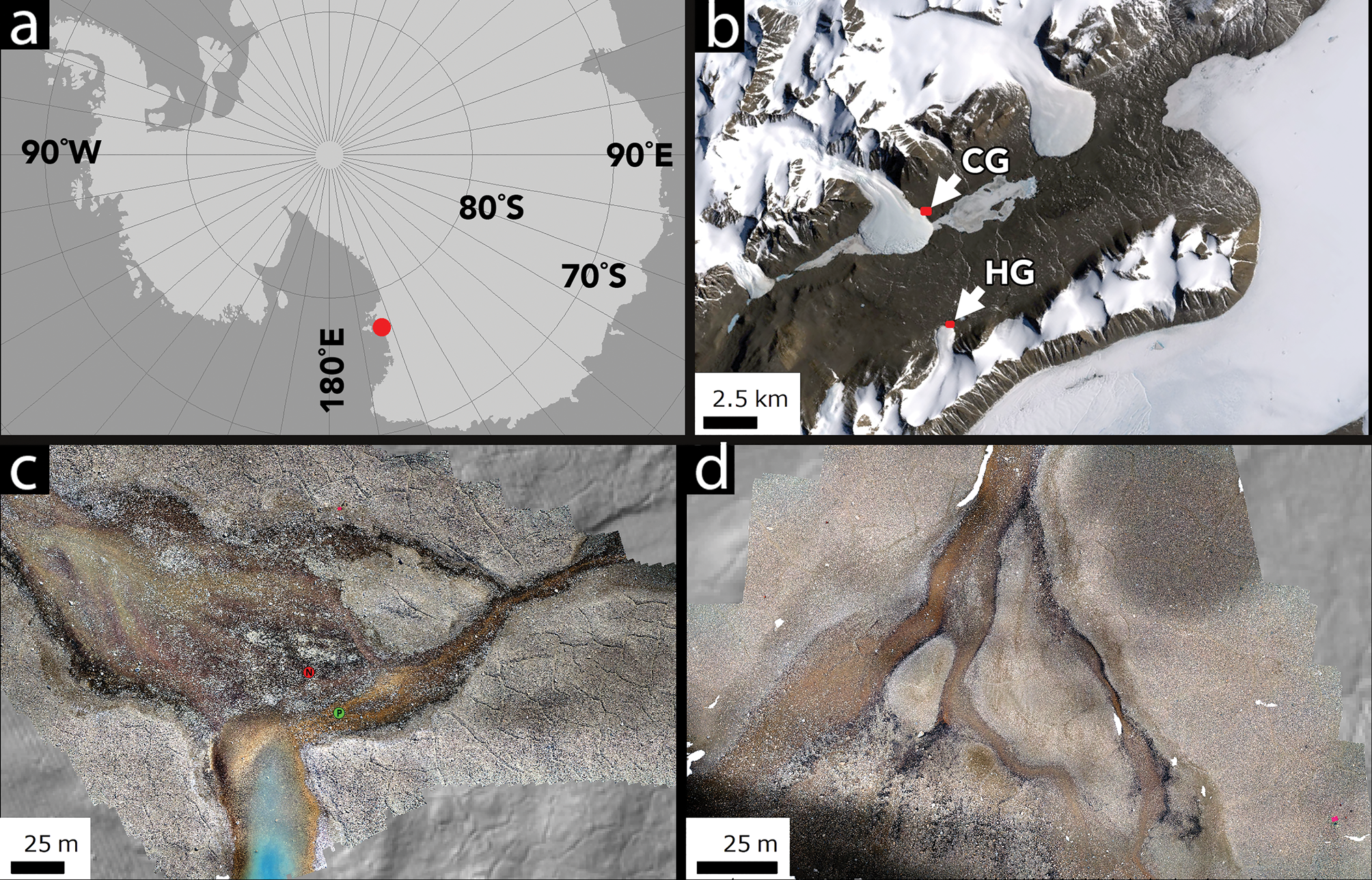
Fig. 1. Location map and context. a. The location of Taylor Valley in the Ross Sea sector of Antarctica. b. The location of Canada Glacier (CG) and Howard Glacier (HG) in eastern Taylor Valley. c. The CG study site. d. The HG study site. Images in c. and d. are orthomosaics generated by UAS flights. b. is a Landsat 7 frame, courtesy of the United States Geological Survey. The green dot labelled P in c. shows the Phormidium mat community sampling site, while the red dot labelled N shows the Nostoc community mat sampling site.
The spectrometer system was mounted on a DJI Phantom 4 Pro UAS using custom 3D-printed side cargo racks that allow unobstructed upwards and downwards looking views. Positioning data for the aircraft were generated using a DJIP4P-R001 GLONASS/GPS module capable of measuring location and altitude above ground level to within ± 1.5 m horizontal and ± 0.5 m vertical, although higher uncertainties are probably during high-latitude operations. Positioning data were collected at ~30 Hz by the aircraft and were averaged into 1 s position reports in order to associate spectral data with positional data. Aircraft roll and pitch averaged -1.0 ± 2.2° and -2.9 ± 4.0°, respectively, producing average off-nadir offsets of 50 cm along the flight track and 18 cm perpendicular to the flight track at 10 m above ground level mission altitude.
Orthomosaics and stereo digital elevation models of the study areas were generated from geotagged UAS photographs and positional data using Agisoft Photoscan Pro. Approximately 20 ground-control point targets were included in the UAS photograph set. Ground control target locations were determined using an Archer Field PC with an external GPS antenna. Orthomosaics were generated with < 1 cm spatial resolution and were orthorectified using the concurrently produced digital elevation model.
Both spectrometer data collection and GPS position data-logging were initiated prior to aircraft lift-off. In order to synchronize the GPS position data with spectrometer measurements, reflectance data were inspected to determine the point at which the red launch tarp ceased dominating the STS-VIS spectra. This spectrometer data time-stamp was correlated with the first UAS GPS point immediately adjacent to the launch tarp based on the orthophoto mosaic and the UAS position log. Synchronization between reflectance and positioning datasets was verified by ensuring that the spectrometer response returned to red tarp reflectance at the GPS point when the aircraft crossed back over the launch tarp at the end of the mission.
Ground-based reference spectra were collected over orange and black mat reference mats at eight target sites (e.g. Figs 2 & 3) and an airborne reflectance transect was conducted to evaluate linkages between ground-based and airborne spectra (Fig. 4). Mats were classified in the field using the shorthand classification by colour from Howard-Williams et al. (Reference Howard-Williams, Vincent, Broady and Vincent1986), but we recognize that most MDV mats contain a number of cyanobacterial taxa as well as other bacteria (Howard-Williams et al. Reference Howard-Williams, Vincent, Broady and Vincent1986, Jungblut et al. Reference Jungblut, Hawes, Mountfort, Hitzfield, Dietrich and Burns2005). Airborne and ground-based spectra were integrated over ~10 s per sample site (~100 scans). Based on sediment background spectra shape, we calculated a range of candidate unitless spectral parameters for analysis. Four were site-specific and were selected based on spectral shape at the site: MEANRED (average reflectance from 549.95 to 800.00 nm), RSLOPE (spectral slope in the red and near-infrared (NIR) range from 710.30 to 800.00 nm, calculated via least squares regression), BSLOPE (spectral slope in the blue range from 549.95 to 600.04 nm, calculated via least squares regression) and S56 (spectral slope in the blue-green transition from ~500.00 to 600.00 nm). We also computed two unitless spectral parameters based on previous efforts to detect polar microbial mats: B6 and NDVIp. B6 is a band depth parameter designed to detect a classic spectral absorption feature at ~667 nm common to orange and black mats that is associated with chlorophyll a (Weaver & Wrigley Reference Weaver and Wrigley1994) and, to a lesser extent, with low red light reflectance of biliproteins (Figs 2 & 3) (Prezelin & Boczar Reference Prezelin, Boczar, Round and Chapman1986). NDVIp is a parameter based on the NDVI, but it is considered ‘partial’ because it only contains approximately five channels of reflectance measurements in the true NIR range owing to the limited spectral range of the UAS-borne detector. B6 is calculated as in Eq. (1):
 $$ \eqalign{ {\rm B}6 &= ( {{\rm mean\ reflectance}) \;({683.5\ndash 687.5{\rm nm}} ) } \cr&\quad {\hbox -} \; { {\rm mean\ reflectance\ }( {664.2\ndash 668.2{\rm nm}} ) } ) / \cr&\quad \, {\rm mean\ reflectance\ } ( {683.5\ndash 687.5{\rm nm}} ) $$
Fig. 2. Reflectance spectrum of an orange Phormidium mat collected using the STS-VIS from the ground. Spectrum is a 10 scan stack filtered through a 10 channel moving average. Grey shading indicates one standard deviation of the reflectance over the averaging window. a and b are spectral regions used in the calculation of the B6 index. Red and NIR indicate the wavelength regions averaged together to produce a partial NDVI equivalent parameter (NDVIp).

Fig. 3. Reflectance spectrum of a black Nostoc mat collected using the STS-VIS from the ground. Spectrum is a 10 scan stack filtered through a 10 channel moving average. Grey shading indicates one standard deviation of the reflectance over the averaging window. a and b are spectral regions used in the calculation of the B6 index. Red and NIR indicate the wavelength regions averaged together to produce a partial NDVI equivalent parameter (NDVIp).

Fig. 4. a. Aerial images of scan positions used for band parameter determination transect. Circles indicate approximate position of spectra. From 1 to 5, positions were selected to be free of mat material, to be a mixture of rocks and mats, to be mat dominated, to be a mixture of rocks plus mat and to be free of mats. b. Example spectrum (orange mat) showing wavelength ranges used in the calculation of spectral parameters. Worldview-3 bandpasses are shown for comparison. c. Reflectance parameters calculated as a function of distance across the transect. Only B6 rises to a maximum where mats are dominant.
B6 is the absorption depth at the lowest reflectance point of the 667 nm absorption feature relative to the reflectance on the red side of the absorption feature (Figs 2 & 3). Averaging spectral channels over the absorption centre and immediately outside the absorption feature acts as a boxcar style filter, reducing noise.
NDVIp is calculated as in Eq. (2):
 $$\lpar {{\rm NIR\ } \hbox {-} \;{\rm RED}} \rpar /\lpar {\rm NIR} + {\rm RED}\rpar $$
where RED is the mean of reflectance from 630 to 690 nm and NIR is the mean of reflectance from 770 to 800 nm.
For comparison between spectroscopic measurements and orthomosaic measurements, RGB digital number (DN) values were extracted from the colour orthomosaics at the locations of each spectroscopic reflectance stack. Colour DN values are blended across the full orthomosaic scene during mosaic generation to provide a uniform but qualitative measure of brightness with a common baseline determined by average illumination conditions during the UAS flight. The DN values can be extracted at independent test points or spectroscopic observation points for comparison between qualitative (DN) and quantitative (reflectance) measurements.
Samples of microbial mat material from neighbouring valleys (-77.80°N, 160.63°E) that were inferred to be inactive were radiocarbon dated at the University of Arizona Accelerator Mass Spectroscopy (AMS) facility and were calibrated using radiocarbon correction from Stuiver & Reimer (Reference Stuiver and Reimer1993) and the Southern Hemisphere radiocarbon calibration of McCormac et al. (Reference McCormac, Hogg, Blackwell, Buck, Higham and Reimer2004). Mats were inferred to be inactive based on a state of near-total desiccation and severe wind abrasion of the mat material. Mat reflectance spectra were collected using the same STS-VIS spectrometer but under broad-spectrum laboratory illumination.
In order to begin to determine how microbial mat community composition maps onto spectral properties and pigment colouration, microbiome analyses were conducted for one orange and one black mat in the study site. For microbiome analysis, mat samples (one of each mat type) were collected ascetically, stored in 50 ml Falcon tubes, transported to New Zealand under temperature-controlled conditions and kept at -20°C prior to DNA extraction. Total DNA was extracted using a MOBIO PowerSoil DNA Isolation Kit (MOBIO Laboratories, USA) following manufacturer protocols. Polymerase chain reaction (PCR) was used to amplify the V4 hypervariable region of the 16S rRNA gene from extracted DNA samples using Ion Torrent fusion primers based on the Earth Microbiome Project primers F515 (5′-GTGCCAGCMGCCGCGGTAA-3′) and R806 (5′-GGACTACVSGGGTATCTAAT-3′). Each reaction consisted of 0.8 μl of bovine serum albumin (Promega Corporation, USA), 2.4 μl of dNTPs (2 mM each; Invitrogen Ltd, New Zealand), 2.4 μl of 10× PCR buffer (Invitrogen Ltd), 2.4 μl 50 mM MgCl2, 0.4 μl of each primer at 10 mM (Integrated DNA Technologies, Inc., USA), 0.096 μl of Taq DNA polymerase (Invitrogen Ltd), 2 μl of genomic DNA (at 2.5 ng μl-1) and molecular-grade ultrapure water. Amplicon sequencing was performed using the Ion Torrent PGM DNA Sequencer with the Ion 318v2 Chip and Ion PGM Sequencing 400 Kit (ThermoFisher Scientific, USA) at the Waikato DNA Sequencing Facility.
The resulting sequences were processed through a custom pipeline. An initial screening step was performed in mothur (Schloss et al. Reference Schloss, Westcott, Ryabin, Hall, Hartmann and Hollister2009) to remove abnormally short (< 250 bp) and long (> 440 bp) sequences. Sequences with long homopolymers (> 7) were also removed. The reads were then quality filtered using UPARSE (Edgar Reference Edgar2013) with a maximum expected error of 1% (fastq_maxee_rate = 0.01) and truncated from the forward primer to 250 bp. Retained sequences were de-replicated, with singleton sequences removed. Next, reads were clustered and chimera-checked using the cluster_otus and uchime2_ref commands in USEARCH, and a de novo database was created of representative operational taxonomic units (OTUs). The OTUs were classified using the RDP Classifier (https://rdp.cme.msu.edu/classifier/classifier.jsp), and 80% was used as the confidence threshold for taxonomic assignments. The taxonomy of dominant cyanobacterial OTUs (> 1% relative abundance in at least one of the mat samples) was confirmed using megablast against the NCBI 16S ribosomal RNA sequence database and cross-referencing the closest representative against the Genome Taxonomy Database (GTDB; http://gtdb.ecogenomic.org). All taxonomic assignments are according to the NCBI Taxonomy Database unless otherwise specified.
Results
We targeted two mat types: ‘Phormidium’, which is typically orange in appearance and commonly found in deeper water, and ‘Nostoc’, which is dark green (close to black) in appearance and usually found in comparatively shallow water (Fig. 1c & d). These mats are not taxonomically homogeneous. Our expectation was confirmed by the results from the 16S rRNA gene PCR amplicon sequences (Table I), which showed that the ‘Phormidium’ mat was dominated (5709 of 29 596 reads, ~20%) by cyanobacterial OTUs affiliated with orders Oscillatoriales (one of which is affiliated with the family Phormidiaceae according to GTDB; Table I) and Synechchococcales, whereas the ‘Nostoc’ mat was dominated (9944 of 29 917 reads, ~33%) by OTUs affiliated with Nostocales and Synechchococcales (mostly distinct from those found in the ‘Phormidium’ mat). The results show a clear difference in the dominant cyanobacterial components of these two microbial mat communities (Fig. 5), and we use the names Phormidium and Nostoc throughout the manuscript to refer to these two mat types, consistent with prior usage of these terms to describe complex and inhomogeneous stream mat communities. At the phylum level, the two mat types harbour broadly similar microorganisms (Fig. 6), dominated (after cyanobacteria) by bacteria affiliated with Proteobacteria and Bacteroidetes.
Table I. Prominent (> 1% relative abundance) cyanobacterial OTUs in representative communities. Percentages inside parentheses indicate similarity of the OTU representative sequence to its closest match in GenBenk.


Fig. 5. Comparison of relative abundances of dominant cyanobacterial taxa in two microbial mat samples representative of ‘Phormidium’ and ‘Nostoc’ types. Note that OTU09 is affiliated with the Phormidiaceae family according to GTDB taxonomy (Table I).

Fig. 6. Comparison of phylum-level bacterial community compositions (inner circle: Phormidium mat; outer circle: Nostoc mat). Groups marked with * are not rendered on the plot due to low abundances. Groups are plotted in order in the legend, clockwise from the top.
On the basis of reflectance measurements made with the STS-VIS spectrometer from the ground, the defining characteristic of Phormidium and Nostoc mats is a notable absorption at ~667 nm (Figs 2 & 3). This absorption is detectable via the B6 parameter from the air (Fig. 4) and most closely matches the observed spatial distribution of mat material in the airborne control transect, increasing with increasing spatial mat presence (Fig. 4). Nostoc mats are of lower reflectivity (darker) at all wavelengths (Fig. 3). Because B6 is a band depth measurement that ratios reflectance at two points in a given spectrum, it cannot be used to discriminate between bright orange Phormidium mats and dark Nostoc mats (Fig. 7).

Fig. 7. B6 parameter strength vs the DN value of a co-located orthoimage. B6 values > ~0.025 are associated with the presence of microbial mats (shaded area) (Figs 8 & 9). However, B6 values are not strongly determinative of Nostoc vs Phormidium, as both mats generate strong ~667 nm absorptions. This motivates the need to generate a secondary parameter for distinguishing mat types.
When mapped spatially, B6 values exceeding ~0.05 are tightly constrained to stream margins and channels where mats are present, while moderate B6 parameter values (0.025–0.050) are associated largely with stream margins where orange Phormidium mats are interspersed with rocks and obstacles (Figs 8 & 9). Low B6 values are confined to rocky interfluves. Similarly, moderate values of NDVIp (0.025–0.050) are recorded in stream channels, with inter-stream dry areas showing low but non-zero (0.01–0.05) values (Figs 8 & 9).

Fig. 8. (Left column) Spatial distribution of B6 parameter values at the Canada Glacier study site. a. Overview of B6 values with locations of other panels. b. High B6 values are concentrated within stream channels in which Nostoc and/or Phormidium are present. c. The B6 absorption reproducibly identifies locations with high concentrations of microbial mats within stream channels. d. B6 identifies mats located in deeper (tens of centimetres) pond water. (Right column) Spatial distribution of NDVIp parameter values at the same locations as in the left column. e. Overview of NDVIp values with locations. f. NDVIp values are low in deep (tens of centimetres) channel thalwegs. g. NDVIp reproducibly identifies microbial mats in stream channels and not in dry, mat-free bank soils. h. NDVIp values are lower than B6 values in deep (tens of centimetres) standing water. Point locations represent average aircraft positions over the 10 spectra collections and are not corrected for roll or pitch. Roll and pitch offsets average 18 and 50 cm, respectively.

Fig. 9. (Left column) Spatial distribution of B6 parameter values at the Howard Glacier study site. a. Overview of B6 values with locations of other panels. b, High B6 values can be detected even in rocky areas in which Nostoc occupies decimetre-scale moats around boulders and cobbles. c. High B6 values are concentrated within stream channels in which Nostoc and/or Phormidium are present. (Right column) Spatial distribution of NDVIp parameter values at the same locations as in the left column. d. Overview of NDVIp values with locations. e. NDVIp values are low in areas with large concentrations of boulders and cobbles. f. NDVIp values are low in channel thalwegs.
NDVIp values differ from B6 most strongly where water depths exceed a few centimetres to tens of centimetres based on field observations of stream and pond depth, but they otherwise share similar magnitudes and spatial extents. Indeed, when examined point by point, NVDIp and B6 are largely co-linear at low values (< 0.05), but diverge at higher values associated with strong B6 features in deeper water (Fig. 10).

Fig. 10. B6 vs NDVIp for one example UAS sortie. B6 and NDVIp are compared point by point. A grey eye-guide line is included in order to highlight the linearity between the two parameters at low values. B6 intensity dramatically increases in regions of Phormidium presence in deeper water where NDVIp does not detect the mats.
Both NDVIp and B6 values are high (> 0.05 and > 0.025, respectively) in stream channel centres and margins where microbial mats are present based on field observations and mat identification on the basis of bright orange and dark black pixels in the colour orthomosaics (Figs 8–10). Both values are low in rocky interfluve environments. High NDVIp values are spatially consistent with the distribution of orange Phormidium mats, but NDVIp values are notably lower than equivalent B6 values in areas with abundant Nostoc mats or within regions with many pebbles or rocks within the spectrometer footprint.
In terms of orthomosaic RGB DN values, Nostoc and Phormidium mats can be distinguished at calibration points that were selected on the basis of mat observations in the field and in the RGB orthomosaics (Figs 11 & 12). Although Nostoc and Phormidium mat DNs are co-linear in all three colour channels, Nostoc mats typically have DNs < 60 and Phormidium points have orthomosaic DN values ranging from 60 to 160 (Figs 11 & 12). The DN differences between mat populations are significant (P < 0.001) and are readily discernible across both field sites (Fig. 12).

Fig. 11. The DN values at calibration points identified in RGB colour orthomosaics known to contain Nostoc and Phormidium mats. The DN values are all strongly collinear across colour bands and across a panchromatic average of the RGB DNs. In all colours, Nostoc are uniformly darker than Phormidium.

Fig. 12. Histogram showing panchromatic RGB-average DN values for Nostoc and Phormidium mats at calibration points. Nostoc are characterized by DN < 60 and are sharply divided from Phormidium, which are characterized by DNs from ~60 to 160. Single-ended analysis of variance values indicate significant differences between these DN populations with P < 0.001.
For comparison, mats inferred to be inactive due to their location around a freeze-dried remnant pond (Fig. 13) show no B6 absorption features. These mats were radiocarbon dated to 934 ± 22 radiocarbon years before present (2σ uncertainty, 735–814 calibrated years before present), suggesting an absence of recent metabolic activity.

Fig. 13. Field setting and reflectance spectrum of an orange microbial mat deposit (inferred to be inactive based on desiccation, abrasion and old radiocarbon age) adjacent to a freeze-dried pond. B6 absorption features are not present.
Discussion
Our measurements indicate that sentinel organisms in the terrestrial Antarctic such as microbial mats can be detected and classified at the ~1 m scale through the combined use of high-spectral-resolution reflectance spectroscopy and high-spatial-resolution imaging. Although microbial mats can be identified by broadband reflectance parameters such as NDVIp, we find that mat-specific parameters such as B6 provide sharper spatial delineation of mat presence and are capable of resolving mats in deeper water, where NIR absorption can otherwise hinder mat detection (Figs 8 & 9).
We propose a straightforward workflow for identifying and classifying microbial mats from hyperspectral and imaging data. Mat presence can be identified through the presence of strong B6 band parameter strength (> 0.05). Extraction of underlying orthoimage colour DN values allows for discrimination between mats. In our study, the DN break point is ~60 (< 60 classifies mats as Nostoc, > 60 classifies mats as Phormidium), although site-specific calibration is recommended, as DN values, unlike reflectance values, are highly sensitive to camera collection settings, illumination, etc.
This workflow and the resulting mat classification at the ~1 m scale are shown in Fig. 14. This workflow allows for the detection and classification of microbial mats using either point-based or imaging reflectance spectrometers, provided the spectral resolution of the spectrometer is sufficient to capture the narrow ~667 nm absorption (Levy et al. unpublished data Reference Levy, Fountain, Obryk, Telling, Glennie and Pettersson2018). By using low-flying point spectrometers or push-broom imagers with sufficient spatial resolution (centimetre scale), we propose that it could be possible to determine annual mat growth or reduction using this method.

Fig. 14. Candidate filtering scheme for identifying Phormidium vs Nostoc mats using combined spectroscopic and RGB data. Blue dots over spectrum collection points indicate mat identification based on the proposed workflow. Note the fine spatial scale at which Nostoc and Phormidium mats can be discriminated between at the ~1 m scale.
Why not just use high-spatial-resolution colour orthomosaics to identify and map sentinel organisms such as mats? In other words, if Nostoc mats are dark black and Phormidium mats are bright orange, is it not enough to characterize mats by colour? Two factors suggest that colour-only mapping is insufficient for detecting the presence of active microbial mats in the MDVs.
First, as is shown in Fig. 15, ‘orange’ and ‘black’ mats span a range of reflectivities over RGB colour space, as measured at known mat locations. When these orthoimage DN values are mapped out spatially, pixels with 60–160 DNs for the red and green channels and 60–140 DNs for the blue channel produce the predicted Phormidium distribution shown in Fig. 15, while pixels with < 60 DNs across all bands are mapped as Nostoc. This colour-only classification significantly over-predicts the distribution of Nostoc mats, incorrectly assigning dark pixels resulting from topographic shadowing as dark mats. Similarly, ‘orange’ pixels that are as orange as field-measured Phormidium mats are over-predicted across sediment surfaces where no mats are present (i.e. outside of streams) but where red-toned sediments are abundant. Use of the combined B6 spectral parameter with colour data, as described above, reduces such false-positive classification by identifying mat-diagnostic chlorophyll absorptions.

Fig. 15. a. and b. show the results of mapping the observed range of Nostoc (green) and Phormidium (blue) RGB DN values from Fig. 12 onto the drone-derived orthoimages. a. is the Howard Glacier site and b. is the Canada Glacier site. Black arrows indicate over-prediction of dark Nostoc mats, especially in shadowed thermal contraction crack troughs, while red arrows indicate over-prediction of Phormidium mats in areas with bright, orange-toned sediment. c. and d. show the underlying orthoimages for comparison.
Second, even when mats are known to be present, spectral mapping may be useful for distinguishing active mats from relict mats. Observations of bright orange mat remnants (Fig. 13) suggest that mat colour pigments may persist over extended periods in some MDV environments, long after mats have ceased engaging in metabolic activity. The detection of sharp B6-related absorptions thus can be interpreted as an indication of ongoing phototrophic activity, while the absence of B6 absorptions may indicate inactive mats. The loss of clear B6 absorptions over multiple years of observations may serve as a potential indictor of changes in mat metabolism or activity and could potentially be developed as a marker of mat stress or changing physical conditions. Conversely, development of a strong B6 absorption feature in relict mats may reflect reactivation of previously inactive communities as regional changes to surface water and groundwater flow begin to modify dormant organisms (e.g. McKnight et al. Reference McKnight, Niyogi, Alger, Bomblies, Conovitz and Tate1999). Detecting these changes in flowing water is facilitated by the B6 parameter, which we show has greater sensitivity in streams and ponds than broadband parameters such as the modified NDVI.
One question emerging from the colour/spectral analysis of these mats is whether the spectral attributes of the mats might change over the course of the season in response to a change conditions (e.g. decreasing insolation, increasing ice cover, a surplus of nutrients, etc.). Our DNA analysis confirms that the two described mat types are dominated by different cyanobacteria, and intra-seasonal change is therefore improbable as the low temperatures in the MDVs should limit turnover at the community level. Nevertheless, the spectral mapping approach outlined in this manuscript would enable us to map microbial mat spectral properties within the summer season and across multiple summers, and it would enable a more refined understanding of microbial mat dynamics in response to changes in environmental conditions.
Conclusions
This work shows that a UAS-borne hyperspectral point spectrometer can be used to determine mat presence, type and activity for microbial mats in the MDVs. While the broadband NDVIp parameter is adequate in many areas for identifying mats, it misses mats in deep (tens of centimetres) water or on highly bouldery surfaces where mats occupy fringing boulder moats. The hyperspectral B6 parameter does not have these shortcomings and produces a greater dynamic range across the sites. When linked with colour orthomosaic image data, B6 band strength can be used to characterize the presence, type and potential activity of sentinel microbial mats in and around MDV streams and lake margins. This approach could be used to monitor change in sentinel organism populations or extents in order to serve as a system proxy for understanding the ecological impact of changing climate conditions in terrestrial Antarctica. Strategic monitoring of sensitive microbial mat communities around the continent could provide an integrative measure of changes in meltwater quantity and quality and potentially even an early warning of ecosystem change.
Acknowledgements
We thank Antarctica New Zealand for logistical support and Anya Noble for assistance with processing the microbial mat samples.
Author contributions
JL conducted fieldwork and spectroscopy data analysis and led paper writing. CKL conducted fieldwork and DNA-based microbiome analysis and assisted in manuscript writing. SCC conducted fieldwork and led the field team, as well participated in manuscript preparation. KJ conducted fieldwork and assisted with spectroscopy data analysis.
Financial support
This work was supported by funding from the New Zealand Ministry of Business, Innovation and Employment to SCC and CKL (UOWX1401, the Dry Valley Ecosystem Resilience (DryVER) project). JL was supported in part by the Colgate University Faculty Development Council and by NSF OPP award 1847067.
Details of data deposit
DNA sequencing data have been deposited at the Sequence Read Archive under PRJNA607309.


