


Introduction
Around the Antarctic continent, even during winter, areas of little or no sea ice cover are regularly observed along the coastline. These coastal polynyas are opened by offshore sea ice drift usually evoked by offshore winds. Thus, their extent and duration are highly dependent on the wind field. The lack of sea ice cover allows for an enhanced atmosphere–ocean interaction and the locally increased heat flux facilitates high sea ice production rates at coastal polynyas. The heat flux also depends strongly on the atmospheric conditions, in particular air temperature and wind speed (Renfrew et al. Reference Renfrew, King and Markus2002, Haid & Timmermann Reference Haid and Timmermann2013).
In the formation process of sea ice, salt is rejected and accumulates in the water column below. On the relatively shallow continental shelves in the marginal seas of the Southern Ocean, this salt enrichment can lead to the formation of very dense water masses. The dense shelf water plays an essential role as a precursor in the production of Antarctic Bottom Water (AABW). The AABW covers most of the world ocean’s abyss and is an essential element in the global circulation.
The Weddell Sea is of particular interest for a study of coastal polynyas since it is considered to be the most productive source region of AABW (e.g. Foldvik & Gammelsrød Reference Foldvik and Gammelsrød1988, Orsi & Bullister Reference Orsi, Johnson and Bullister1999). The wide continental shelves in the south-western Weddell Sea provide ideal surroundings for the production of High Salinity Shelf Water (HSSW), dense shelf water with salinities (S) >34.65 and potential temperatures (θ) <-1.7°C. Due to the perennial sea ice cover and the remoteness of the region, very few measurements are available and modelling is an important tool for gaining insight into the relevant processes, often combined with remote sensing.
Markus et al. (Reference Markus, Kottmeier and Fahrbach1998) investigated polynya area and sea ice production in the Weddell Sea based on satellite passive microwave measurements and a basic thermodynamic model using data from the European Centre for Medium-range Weather Forecasts (ECMWF). More recent studies include Tamura et al. (Reference Tamura, Ohshima and Nihashi2008) and Drucker et al. (Reference Drucker, Martin and Kwok2011) who both used satellite-measured brightness temperatures (ECMWF) and atmospheric reanalysis data (National Centers for Environmental Prediction/National Center for Atmospheric Research, NCEP/NCAR) to calculate sea ice production in Weddell Sea polynyas. Haid & Timmermann (Reference Haid and Timmermann2013) used the Finite-Element Sea ice-Ocean Model (FESOM) to investigate heat flux and sea ice production at coastal polynyas in the south-western Weddell Sea. However, none of these studies systematically assessed the sensitivity of the atmospheric datasets used, although the strong dependence of coastal polynyas on the atmospheric variables makes the choice of the atmospheric data important.
Here, we investigate how atmospheric datasets of different origin and different resolution affect polynya formation in the south-western Weddell Sea, and the consequences for sea ice production and dense water formation. To fulfil this aim, a series of FESOM experiments were conducted using data with different temporal and spatial resolutions from the following sources: the NCEP/NCAR reanalysis (NCEP; daily, 1.875°; Kalnay et al. Reference Kalnay, Kanamitsu, Kistler, Collins, Deaven, Gandin, Iredell, Saha, White, Woollen, Zhu, Chelliah, Ebisuzaki, Higgins, Janowiak, Mo, Ropelewski, Wang, Leetmaa, Reynolds, Jenne and Joseph1996), the Global Model Europe (GME) analysis (6 hourly, 40 km; Majewski & Ritter Reference Majewski and Ritter2002, Majewski et al. Reference Majewski, Liermann, Prohl, Ritter, Buchhold, Hanisch, Paul, Wergen and Baumgardner2002) and two implementations of the regional Consortium for Small-Scale Modelling (COSMO) forecast model (COSMO-15/COSMO-5; hourly, 15 km/5 km; Baldauf et al. Reference Baldauf, Förstner, Klink, Reinhardt, Schraff, Seifert and Stephan2011, Doms et al. Reference Doms, Förstner, Heise, Herzog, Mironov, Raschendorfer, Reinhardt, Ritter, Schrodin, Schulz and Vogel2011). The atmospheric data and the FESOM results were compared for three consecutive winter periods where available (2007–09 for NCEP and GME; only 2008 for the COSMO experiments). Special emphasis is on the south-western Weddell Sea and further on the Coats Land region, situated in the eastern part of the former. The south-western Weddell Sea is important since it is the location of a huge fraction of the Southern Ocean’s dense water formation. The Coats Land region is of interest because within the south-western Weddell Sea only here katabatic winds directly meet the coastline (Ebner et al. Reference Ebner, Heinemann, Haid and Timmermann2014) and thus a high sensitivity to atmosphere model resolution is expected.
Model
The FESOM is a hydrostatic primitive-equation ocean circulation model coupled with a dynamic-thermodynamic sea ice component. The FESOM was developed at the Alfred Wegener Institute and was first described by Timmermann et al. (Reference Timmermann, Danilov, Schröter, Böning, Sidorenko and Rollenhagen2009).
For the parameterization of subgrid-scale processes the model makes use of a vertical mixing scheme dependent on the Richardson number (Pacanowski & Philander Reference Pacanowski and Philander1981), which is combined with additional vertical mixing over a depth dependent on the Monin-Obukhov length as suggested by Timmermann & Beckmann (Reference Timmermann and Beckmann2004). The dedicated equation of state as proposed by Jackett & McDougall (Reference Jackett and McDougall1995) facilitates the calculation of in situ density as a function of potential temperature.
The dynamic-thermodynamic sea ice component uses Parkinson & Washington (Reference Parkinson and Washington1979) thermodynamics and the elastic-viscous-plastic rheology as described by Hunke & Dukowicz (Reference Hunke and Dukowicz1997) and Hunke & Lipscomb (Reference Hunke and Lipscomb2010). The model includes a snow layer, the presence of which affects sea ice growth and melting considerably (Owens & Lemke Reference Owens and Lemke1990). Heat storage within ice or snow is not considered. Instead, linear temperature profiles are assumed in both layers applying the zero-layer approach of Semtner (Reference Semtner1976). Prognostic variables are the mean ice thickness (ice volume per unit area), mean snow thickness (snow volume per unit area), ice concentration and ice drift velocity. Snow and sea ice thickness are both assumed to be evenly distributed over the ice-covered part of each area unit. They can change by melting and freezing processes and by converging sea ice drift. The ice drift, u i , is influenced by wind stress, ocean surface velocity, sea surface slope and internal forces of the ice:
 $$m(\partial /\partial t{\plus}f({\bi k}_{{\bi v}} ^{\ x} )){\bi u}_{{\bi i}} =A\left( {\bitau _{{{\bi ai}}} \,{\hbox -}\,\bitau _{{{\bi io}}} } \right){\plus}{\bi F} \, {\hbox -} \, mg\ \bnabla H_{{\rm s}} ,$$
where m is the mass of ice plus snow per unit area, f is the Coriolis parameter, k v is the unit vector in vertical direction, A is the sea ice concentration, τ ai is the wind stress, τ io is the ice/ocean stress, F represents the effect of the internal stresses in the sea ice as a function of ice drift, thickness and concentration, g is the gravitational acceleration, and H s is the sea surface elevation obtained from the ocean component of FESOM.
While the mass flux associated with precipitation and evaporation in the model is given by or calculated from variables of the atmospheric dataset, the thermodynamic part of the sea ice model recalculates the heat flux components. The short wave radiative heat flux, Q sw, is given by the empirical formulation:
 $$\eqalignno{ Q_{{{\rm sw}}} = \ & (\alpha \,{\hbox -} \, {\rm 1}){\times}(S_{0} {\rm cos}^{{\rm 2}} \zeta {\times}({\rm 1}\,{\hbox -}\,0.{\rm 6}{\times}C^{{\rm 3}} )){\times}(({\rm cos}\zeta {\plus}{\rm 2}.{\rm 7)} \cr & {\times}e_{{{\rm v},{\rm a}}} {\times}{\rm 1}0^{{{\hbox -}{\rm 5}}} {\plus}{\rm 1}.0{\rm 85}{\times}{\rm cos}\zeta {\plus}0.{\rm 1})^{{{\hbox -}{\rm 1}}} , $$
where α is the surface albedo, S 0 is the solar constant, ζ is the angular zenith distance of the sun, C is the relative cloud cover, and e v,a is vapour pressure in the air in Pa.
The long wave radiative heat flux, Q lw, is:
 $$Q_{{{\rm lw}}} ={\varepsilon}_{{\rm S}} \sigma _{{\rm B}} T_{\!\!{\rm S}} ^4-{\varepsilon}_{{\rm a}} \sigma _{{\rm B}} T_{\!\!{\rm a}} ^4,$$
where the emissivities of the ice/ocean surface ε S=0.97 and the atmosphere ε a=0.765+0.22×C 3 (König-Langlo & Augstein Reference König-Langlo and Augstein1994), σ B is the Stefan-Boltzmann constant, T S is the surface temperature and T a is the air temperature at 2 m height.
The latent heat flux, Q l, is determined by:
 $$Q_{{\rm l}} =L_{{\rm e}} \rho _{{\rm a}} \!C_{{\rm l}} u_{{{\rm 1}0}} (q_{{\rm S}} -q_{{\rm a}} ),$$
where L e is the heat of evaporation, ρ a is the density of air, C l is the heat transfer coefficient, u 10 is the ten-metre wind speed, and the specific humidity at the surface and at 2 m height are represented by q S and q a, respectively.
The sensible heat flux, Q S, is:
 $$Q_{{\rm S}} =c_{{\rm p}} \rho _{{\rm a}} \!C_{{\rm S}} u_{{{\rm 1}0}} (T_{{\rm S}} -T_{{\rm a}} ),$$
where c p is the specific heat of air and C S is the heat transfer coefficient for sensible heat over ice/snow and water (Parkinson & Washington Reference Parkinson and Washington1979). The transfer coefficients of sensible and latent heat are taken as C l=C S=1.75×10⁻³.
Heat flux, salt flux and momentum flux are transferred between the ocean and sea ice model components after each 3 minute time step. The same global, unstructured surface grid is used for both model components. Its horizontal resolution ranges from 2.5° in the mid-latitude open ocean to 3–5 km at the western Weddell Sea coastline. In vertical direction, 37 depth levels (z-levels) were installed. The uppermost layer has a thickness of 10 m, followed by layers of 15 m, 20 m, 25 m and 30 m in the upper 100 m. The layer thickness increases with depth to a maximum of 250 m, reached at depth 2500 m. The topographical dataset RTopo-1 (Timmermann et al. Reference Timmermann, Le Brocq, Deen, Domack, Dutrieux, Galton-Fenzi, Hellmer, Humbert, Jansen, Jenkins, Lambrecht, Makinson, Niederjasper, Nitsche, Nøst, Smedsrud and Smith2010) was used to create the model’s bathymetry. Further details are found in Haid & Timmermann (Reference Haid and Timmermann2013).
Atmospheric datasets
The NCEP/NCAR reanalysis dataset is used for a 30 year simulation that was initiated on 1 January 1980 with data from the Polar Science Center Hydrographic Climatology (Steele et al. Reference Steele, Morley and Ermold2001). Only the last 3 years of this simulation (2007–09) are discussed here. The GME experiment is branched off from the NCEP run on 1 April 2007, and both COSMO experiments are branched off from the GME experiment on 1 March 2008. In all experiments, the variables of the forcing datasets are interpolated in space from the grid points on which they are provided to the FESOM surface grid points and in time between the points at which they are given to every individual FESOM time step.
National Centers for Environmental Prediction/National Center for Atmospheric Research reanalysis
Atmospheric forcing for 1980–2009 was derived from the NCEP/NCAR reanalysis dataset (Kalnay et al. Reference Kalnay, Kanamitsu, Kistler, Collins, Deaven, Gandin, Iredell, Saha, White, Woollen, Zhu, Chelliah, Ebisuzaki, Higgins, Janowiak, Mo, Ropelewski, Wang, Leetmaa, Reynolds, Jenne and Joseph1996). This is a global dataset with a horizontal resolution of 1.875°. Daily datasets of ten-metre wind velocity, two-metre air temperature, sea level air pressure, two-metre specific humidity, precipitation rate, relative cloud cover and latent heat flux (Q l NCEP) are used. From these quantities, evaporation mass flux (E) in FESOM was calculated as:
 $$E=Q_{{\rm l}} ^{{\ \,\rm NCEP}} (L_{{\rm e}} \rho _{{\rm w}} )^{{{\hbox -}{\rm 1},}} $$
where L e is the latent heat of evaporation of water and ρ w the density of water.
Global Model Europe
The GME is a global weather prediction model developed by the national meteorological service in Germany, the Deutscher Wetterdienst (DWD). Previously described by Majewski & Ritter (Reference Majewski and Ritter2002) and Majewski et al. (Reference Majewski, Liermann, Prohl, Ritter, Buchhold, Hanisch, Paul, Wergen and Baumgardner2002). The model is based on an almost uniform icosahedral-hexagonal grid with a horizontal resolution of 40 km. A 6 hourly dataset covering April 2007 to December 2009 was interpolated to a regular grid with 0.5° spacing. It includes ten-metre wind velocity, two-metre air temperature, two-metre dew point temperature, sea level air pressure, precipitation rate and relative cloud cover. To obtain the variables required by FESOM, the vapour pressure and the specific humidity are calculated from the dew point temperature. Then the evaporation is determined from the latent heat flux, given by Eq. (4).
Consortium for Small-Scale Modelling forecast model
The COSMO model (Baldauf et al. Reference Baldauf, Förstner, Klink, Reinhardt, Schraff, Seifert and Stephan2011, Doms et al. Reference Doms, Förstner, Heise, Herzog, Mironov, Raschendorfer, Reinhardt, Ritter, Schrodin, Schulz and Vogel2011) is a further development of the Lokalmodell of DWD (Doms & Schättler Reference Doms and Schättler2002, Doms et al. Reference Doms, Förstner, Heise, Herzog, Raschendorfer, Schrodin, Reinhardt and Vogel2005). It is a regional non-hydrostatic atmospheric model with terrain-following vertical co-ordinates. The version of COSMO used here (4.11) is optimized for polar conditions and modified with a sea ice model as described in Schroeder et al. (Reference Schroeder, Heinemann and Willmes2011).
Runs with two high-resolution configurations of the COSMO model were performed for March to August 2008 with hourly values. The first COSMO dataset was obtained from a simulation with 15 km horizontal resolution (COSMO-15), and the second configuration has a horizontal resolution of 5 km (COSMO-5). For more details on COSMO and configurations see Ebner et al. (Reference Ebner, Heinemann, Haid and Timmermann2014).
The data was supplied to FESOM on a regular grid with 0.125° (COSMO-15) and 0.05° (COSMO-5) spacing. The domains of the regional atmospheric models providing the COSMO-15 and COSMO-5 datasets and the areas within which the data was applied to FESOM are shown in Fig. 1a. While COSMO-15 receives its boundary conditions from GME, COSMO-5 is run with boundary conditions from COSMO-15 (double-nesting). The COSMO-5 and COSMO-15 model versions are identical in all aspects apart from the model domain, resolution and boundary conditions.
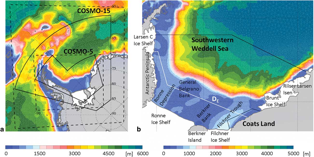
Fig. 1a Bathymetric map depicting the domains of the two implementations of the regional COSMO model (dashed lines) and the areas where the data is applied as forcing to the FESOM model (solid lines). b. Bathymetric map of the study area depicting the south-western Weddell Sea and and Coats Land regions (black lines) and the demarcation line DE (white line). Bathymetry is derived from the Rtopo-1 dataset (Timmermann et al. Reference Timmermann, Le Brocq, Deen, Domack, Dutrieux, Galton-Fenzi, Hellmer, Humbert, Jansen, Jenkins, Lambrecht, Makinson, Niederjasper, Nitsche, Nøst, Smedsrud and Smith2010).
For both COSMO realizations, as with GME, the variables provided are ten-metre wind velocity, two-metre air temperature, two-metre dew point temperature, sea level air pressure, precipitation rate and relative cloud cover. The calculation of the required quantities for FESOM is the same as for the GME forcing data.
In the COSMO-forced FESOM runs, GME forcing was not only applied during the period 1 April 2007 to 29 February 2008, but the regional model data was also complemented by the GME dataset to achieve global coverage from March to August 2008.
Mean patterns
To analyse the large-scale differences between the forcing datasets, maps of the major forcing variables, wind and air temperature, and the resulting sea ice concentration and ice production per unit area are presented in Figs 2–5 showing the mean for April to August in 2007–09 for NCEP and GME forcing and for 2008 for COSMO-15 and COSMO-5 forcing. A quantitative overview is given in Table I.

Fig. 2 Wind field maps averaged over April to August. a.–c. NCEP analysis and d.–f. GME analysis for 2007–09. g. & h. COSMO-15 and COSMO-5 forecasts for 2008. i. Difference between COSMO-5 and COSMO-15 forecasts. The arrows depict the vector mean and the background colours show the mean wind speed. Please note that i. uses a different scale. Units are the same for all plots.
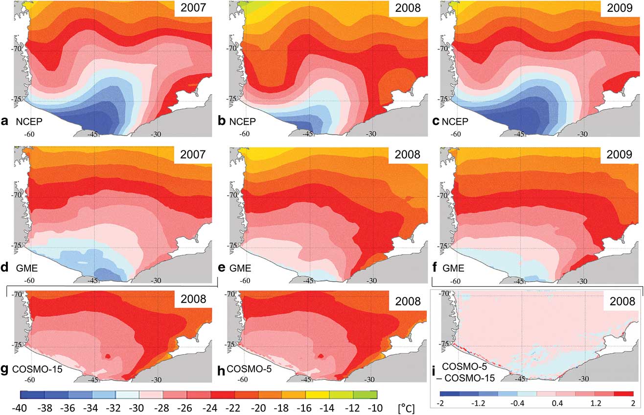
Fig. 3 Air temperature maps averaged over April to August. a.–c. NCEP analysis and d.–f. GME analysis for 2007–09. g. & h. COSMO-15 and COSMO-5 forecasts for 2008. i. difference between COSMO-5 and COSMO-15 forecasts. Please note that i. uses a different scale. Units are the same for all plots.
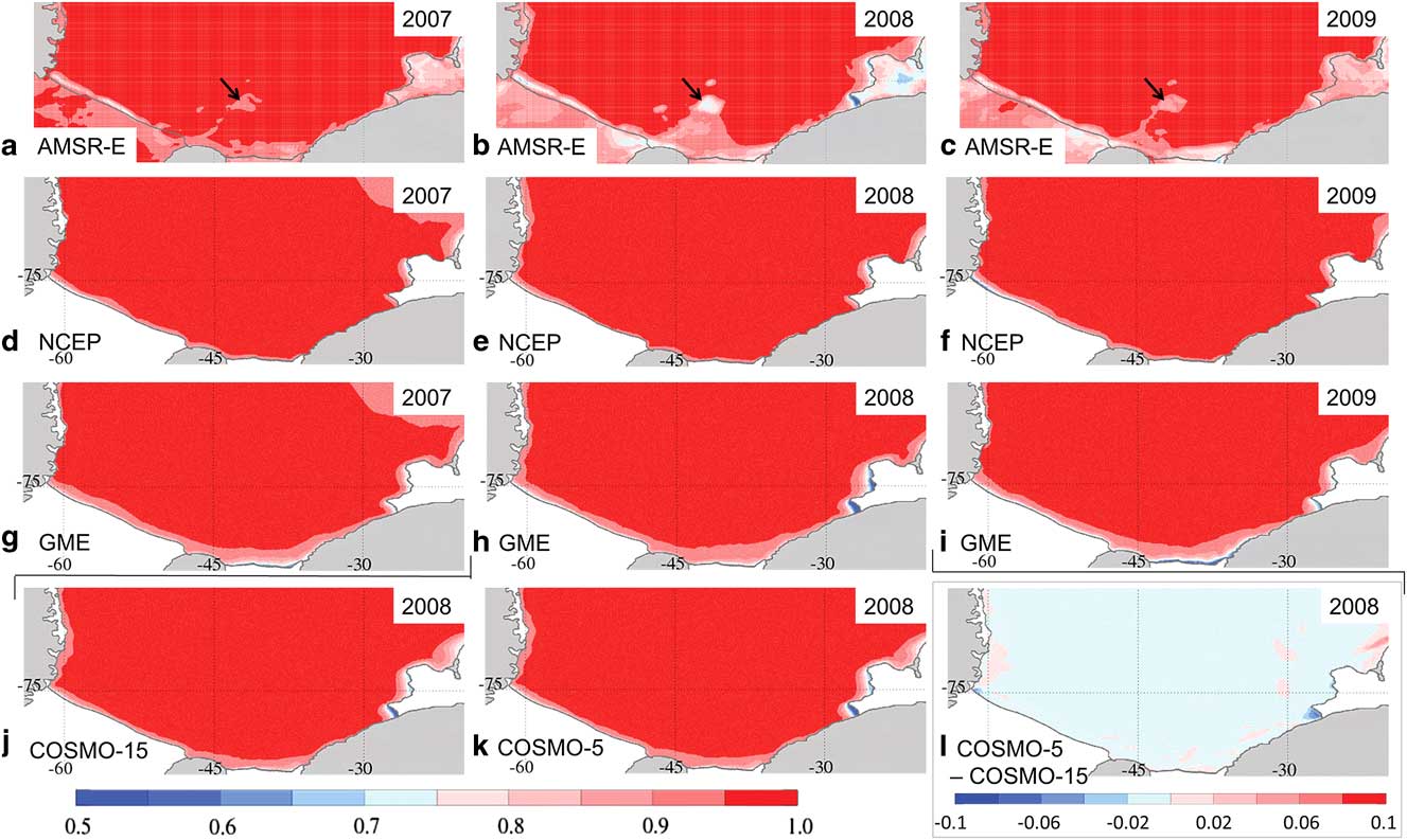
Fig. 4 Sea ice concentration maps averaged over April to August. a.–c. AMSR-E observations (black arrows mark the location of iceberg A23). d.–f. NCEP analysis and g.–i. GME analysis for 2007–09. j. & k. COSMO-15 and COSMO-5 forecasts for 2008. l. Difference between COSMO-5 and COSMO-15 run. Please note that l. uses a different scale. Since the ice shelf fronts are subject to change, the coastline drawn may differ from the actual location of the coastline in the depiction of satellite data.
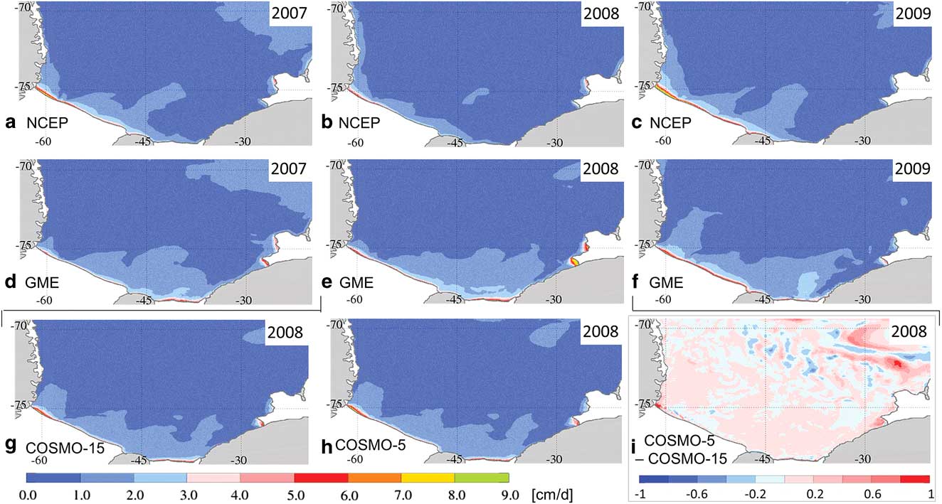
Fig. 5 Sea ice production maps averaged over April to August. a.–c. NCEP analysis and d.–f. GME analysis for 2007–09. g. & h. COSMO-15 and COSMO-5 forecasts for 2008. i. Difference between COSMO-5 and COSMO-15 run. Please note that i. uses a different scale. Units are the same for all plots.
Table I Number of polynya days and mean polynya area, wind speed, air temperature and ice production in the south-western Weddell Sea for April to August in 2007–09. Polynya area is provided as a percentage of the region’s area and polynya sea ice production is provided as a percentage of the regional sea ice production.

Ten-metre wind field
The wind field over the south-western Weddell Sea in the 5 month winter mean (Fig. 2) reveals substantial differences between the forcing datasets. In the NCEP data, for all 3 years, strong easterly to north-easterly winds dominate the area around Brunt Ice Shelf. A lesser maximum with south-westerly winds is found at the (south-)western coastline. In the space between the two maxima, the winds of the NCEP forcing are generally weak (<4.5 m s-1).
In contrast, in the GME forcing almost the entire area features mean wind speeds >4.5 m s-1 with a tendency for increased wind speeds over the open ocean. In all 3 years, a minimum is found at the western coastline, where southerly winds occur as expected from observations (Schwerdtfeger Reference Schwerdtfeger1975, Parish Reference Parish1983). In 2007, the coastline of Coats Land features very weak winds. At this location, a wind speed reduction is also indicated in 2009, although less distinct. However, in 2008 a strong wind speed maximum covering the northern part of the Coats Land coastline next to Brunt Ice Shelf is found.
Furthermore, in 2008 the GME wind speed maximum over the open ocean was exceptionally strong in both mean wind speed and vector mean. The flow connecting the two maxima results in a cyclonic pattern, the centre of which is located at roughly 28°W, 72°S. The NCEP data also features a cyclonic wind pattern in 2008, but it is weaker, larger in extent and centred further west (43°W, 73°S).
The distinctions which set the 2008 wind field apart from other years may be connected to the La Niña/ positive Southern Oscillation Index (SOI) event in this year. The strengthening of cyclonic air flow in the south-western Weddell Sea correlates well with the local wind anomalies pattern found by Kwok & Comiso (Reference Kwok and Comiso2002) for a positive SOI scenario.
The two COSMO datasets feature almost identical wind fields. The pattern is also very similar to the GME wind pattern; however, the mean wind speeds are significantly lower in almost the entire area, except for narrow stretches along the fronts of the Filchner and Ronne ice shelves.
Differences in the wind field between the two COSMO datasets are small, but in general the higher resolved COSMO-5 model results in higher wind speeds. This effect is enhanced along the coastline and most significant where the coastline is not bordered by ice shelves and the influence of small-scale topography is strongest.
Two-metre air temperature
For the air temperatures (Fig. 3), the large-scale distributions in NCEP and GME forcing are similar; with warm air temperatures in the north, which decrease toward a minimum near Berkner Island. Along the eastern coast comparatively warm air temperatures (often with a gradient in a northward direction) are shown. However, in the NCEP data strong undulations are visible (probably related to the spectral method used in the NCEP/NCAR reanalysis model), while the GME temperatures feature a much smoother picture. Further, the minimum in the NCEP temperatures is more pronounced and located to the west of Berkner Island, while it is weaker and to the east of the island in the GME data. In both datasets, 2008 is the warmest of the 3 years, as is expected during a La Niña/ positive SOI event (Kwok & Comiso Reference Kwok and Comiso2002, Yuan Reference Yuan2004).
The two COSMO implementations, again, have very similar results and the pattern resembles that of the GME temperatures. However, the minimum at the southern ice shelf front is slightly less pronounced than in the GME data and located west of Berkner Island. The air at and downstream of the Brunt polynyas (and the polynya at Riiser-Larsen Ice Shelf) experienced warming from the open water areas and local temperature maxima are visible. A southward indent of elevated temperatures in the COSMO air temperature fields, which is also visible in the GME data, is connected to the signature of the grounded iceberg A23 (c. 42°W, 76°S) and the surrounding polynyas, which are represented as areas of reduced ice concentration in the lower boundary conditions of the COSMO model.
In both COSMO data fields and less pronounced in the GME air temperatures, a narrow stretch of very cold air temperatures is visible in front of the Ronne Ice Shelf (where it is best visible, but not limited to) followed by small local maxima of the temperature. The cold temperatures are spurious and result from the use of different land masks in the atmospheric and oceanic models, they represent areas where the atmospheric model still assumes the presence of an ice shelf. The small temperature maxima indicate the presence of polynyas at the ice shelf front in COSMO’s forcing dataset. It is this very narrow band of polynyas along the coastline where the largest differences between COSMO-15 and COSMO-5 temperatures are found. COSMO-5 usually, but not at all locations, features slightly higher temperatures.
Sea ice concentration
In the sea ice concentration fields from Advanced Microwave Scanning Radiometer for EOS (AMSR-E) data (Spreen et al. Reference Spreen, Kaleschke and Heygster2008; Fig. 4a–c), no mask is used to cover the data over the ice shelves in order to underline the characteristics and potential errors of the satellite data. Areas of ice shelves, icebergs or fast ice can lead to similar signals as low sea ice concentration in the AMSR-E data (best visible in Fig. 4b). Therefore, difficulties in the interpretation arise especially at the changeable ice shelf edge if the correct location is unknown.
The most striking features in the satellite data are the Ronne polynya, the iceberg A23 (black arrows in Fig. 4a–c) with a fast ice bridge connecting it to the southern coastline, and the polynyas in front of Brunt Ice Shelf. The presence of A23 and its influence on the surrounding sea ice (Markus Reference Markus1996) preclude a robust decision on which forcing performs better in the area of the Filchner Ice Shelf. Unfortunately, this is the area where the sea ice concentrations differ most between the model runs. While in the NCEP run in all 3 years only a very weak and narrow signature of reduced sea ice concentration is visible in front of Filchner Ice Shelf due to the weak winds, the GME run features the widest and (except in 2008) strongest polynya signature here, which is created by the strong south-easterly winds in this area (Fig. 2).
The Ronne polynya in the NCEP run is widest at its western border and narrows toward the east. This is similar to the signature in the satellite observations, while the GME forcing creates a belt of reduced sea ice concentrations of almost invariable width along the Ronne Ice Shelf front, which continues and widens along the Filchner Ice Shelf front and slowly narrows at the Coats Land coastline.
The polynyas off Brunt Ice Shelf show little interannual variability in the NCEP run (except for a slight weakening in 2009). In the GME run, while overestimating polynya activity compared to the AMSR-E observations, interannual variations are reproduced well (weakest polynyas in 2007, strongest in 2008). Furthermore, the often blurred shape of the polynya areas in this region is recreated in the GME run, although not always matching the observations in detail.
For 2008, the COSMO runs yield the best fit to the AMSR-E observations. Although both COSMO runs underestimate the width of the Ronne polynya (it is slightly more pronounced in the COSMO-5 run, especially in the western corner), the eastern polynyas are very well recreated with a strong signature of the southern Brunt polynya (stronger in COSMO-5) and a less active northern Brunt polynya. Even the blurred western edge of the polynya in front of Riiser-Larsen Ice Shelf can be found in both the satellite observations and the COSMO runs. Here the COSMO-5 run features a higher ice concentration than the COSMO-15 run and is, again, closer to the observations. Along Filchner Ice Shelf the COSMO runs feature a pattern similar to the GME run; however, it is significantly reduced in extent and intensity. The sea ice concentrations in both COSMO runs are very similar. However, the differences generally make the COSMO-5 results a slightly better match to the observations.
Sea ice production
In the NCEP run, the highest freezing rates are found at Ronne polynya (Fig. 5), followed by the northern Brunt polynya. The GME run features the southern Brunt polynya with higher freezing rates than the northern Brunt polynya and besides the Ronne polynya an additional maximum in front of Filchner Ice Shelf. Between years, the relative importance of those regions shifts in the GME run (2007: maxima at Filchner Ice Shelf front and southern Brunt polynya, 2008: maxima at Brunt polynyas, 2009: maximum at Ronne polynya); while in the NCEP run, the relations appear stable and only overall intensity changes (minimum in 2008, maximum in 2009). The only exceptions in the NCEP simulation are the western polynyas at the Antarctic Peninsula coastline, which feature maximum ice production in 2008.
In summary, most of the sea ice production in the NCEP run occurs on the western part of the continental shelf (connected to Ronne polynya), while in the GME run (except in 2009) it occurs on the eastern part of the shelf at the Brunt polynyas and in front of Filchner Ice Shelf.
The two COSMO runs again yield very similar results. The distribution of the ice production also resembles the results of the GME run. However, while the Ronne polynya west of General Belgrano Bank (c. 55°W) features higher freezing rates than in the GME run, all areas east of 55°W have lower sea ice production, especially the Brunt polynyas. As a result, the highest freezing rates in the COSMO runs are found at Ronne polynya and the sea ice production along the coastline is more evenly distributed than in the NCEP or GME runs.
The largest differences in the sea ice production between the two COSMO runs are found over the deep ocean, where small differences in the localization of convective cells cause a high local impact on the sea ice production. However, on a larger scale these differences cancel each other out almost completely. Over the continental shelf, the most dominant differences are again linked to the coastal polynyas. In the COSMO-5 run, higher ice production is found in the Brunt polynyas and the Ronne polynya (especially the western corner) and also a more localized ice production with higher values close to the coastline and lower values slightly farther offshore along the Ronne and Filchner ice shelves.
Spatial-mean sea ice production
A comparison of the mean sea ice production from April to August 2008 in the south-western Weddell Sea (see Fig. 1b for the area of interest) and in the polynyas within the south-western Weddell Sea shows that while sea ice production per unit area in polynyas (blue line in Fig. 6a–c; Table I) exceeds the regional mean (red line in Fig. 6a–c; Table I), the bulk of the sea ice volume (Fig. 6d–f) does not originate from polynyas due to the small total area. The temporal variations reveal that anomalies generally occur consistently across all four datasets, but the magnitude of the anomalies can differ strongly. Great coherence is shown between simulations, especially in regional sea ice volume produced (red line in Fig. 6d–f) and polynya sea ice production after day 170 (blue line in Fig. 6a–c). However, in the polynya sea ice production during the April and May there are substantial differences between the simulations. For example, a maximum on day 112 occurs in the GME and COSMO experiments but this event is not reflected in the NCEP results. The NCEP polynya sea ice production features a maximum on days 154/155, which cannot be found with a comparable intensity in the GME results. The COSMO results yield values between those of the NCEP and GME forced simulations.
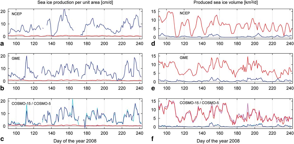
Fig. 6a.–c Time series of sea ice production per unit area and d.–f. accumulated sea ice production in the south-western Weddell Sea for April to August 2008; mean regional (red) and polynya ice production (blue; in a.–c. only when polynyas exist). Light blue and light red curves in c. and f. depict the COSMO-5 values.
The mean regional sea ice production is lowest in the NCEP run (Table I). The GME run on average has higher values than the COSMO-5 results, which in turn feature a higher sea ice production per unit area than the COSMO-15 results. However, all the values are within a small range of 0.06 cm d-1 m-2 around a mean of 0.51 cm d-1 m-2 (Table I).
In contrast to the mean regional sea ice production, the polynya sea ice production per unit area is highest in the NCEP simulation (closely followed by the GME results), while the COSMO-15 experiment yields the lowest numbers (Table I). For the polynya sea ice volume produced, the GME forcing results in the highest value (101 km3), as it has both the largest mean polynya area (9800 km2) and a high mean polynya ice production per unit area (6.8 cm d-1 m-2) due to the highest mean wind speed (5.7 m s-1). The NCEP run features the lowest mean wind speed by a clear margin and, therefore, typically the smallest and least frequent polynyas. In total ice volume and as a percentage of the regional sea ice production, the polynyas in the COSMO runs contribute least.
The Coats Land region in the south-eastern corner (Fig. 1b) is the only region in the south-western Weddell Sea where mountains border the ocean without being separated by ice shelves. Therefore, katabatic winds originating from the mountain slopes reach the coastline with little deceleration. The spatial resolution of the atmospheric model is thought to be crucial for the representation of katabatic winds (Jourdain & Gallée Reference Jourdain and Gallée2011). Therefore, it was expected that the four model runs would yield substantially different results here.
In the Coats Land region (Table II), the NCEP run features hardly any polynyas, because the mean wind field (Fig. 2a–c) in this region is parallel to the coast (causing ice drift toward the coastline), and also has the lowest variability compared to the other atmospheric datasets. In the GME run, frequent and very large polynyas at the Coats Land coastline (Fig. 4g–e) are facilitated by the more easterly winds. The COSMO runs, which have the finest spatial resolution in the atmospheric forcing, feature less frequent and smaller polynyas than the GME run and the resulting polynya ice volume is much smaller, which suggests that the polynya formation and sea ice production in the Coats Land region is overestimated in the GME simulation.
Table II Number of polynya days and mean polynya area, wind speed, air temperature and ice production in the Coats Land region for April to August 2007–09. Polynya area is provided as a percentage of the region’s area and polynya sea ice production is provided as a percentage of the regional sea ice production.
Furthermore, along the Antarctic Peninsula, we find a high mountain range close to the coastline. Therefore, the local coastal wind field is strongly influenced by the channelling effect of the nearby valleys. This entails that the performance of the atmospheric model depends essentially on its capability to resolve the orography. As an example, the coastal polynyas adjoining the southern part of the Antarctic Peninsula on 29 August 2008 (Fig. 7) feature significant differences between the experiments conducted with different forcing data. The satellite data (Fig. 7a) shows coastal polynyas open between 71.5°S and 75°S. The widths vary strongly and reach maxima at ≈72°S, ≈73.5°S and, although with less intensity, ≈74.5°S.
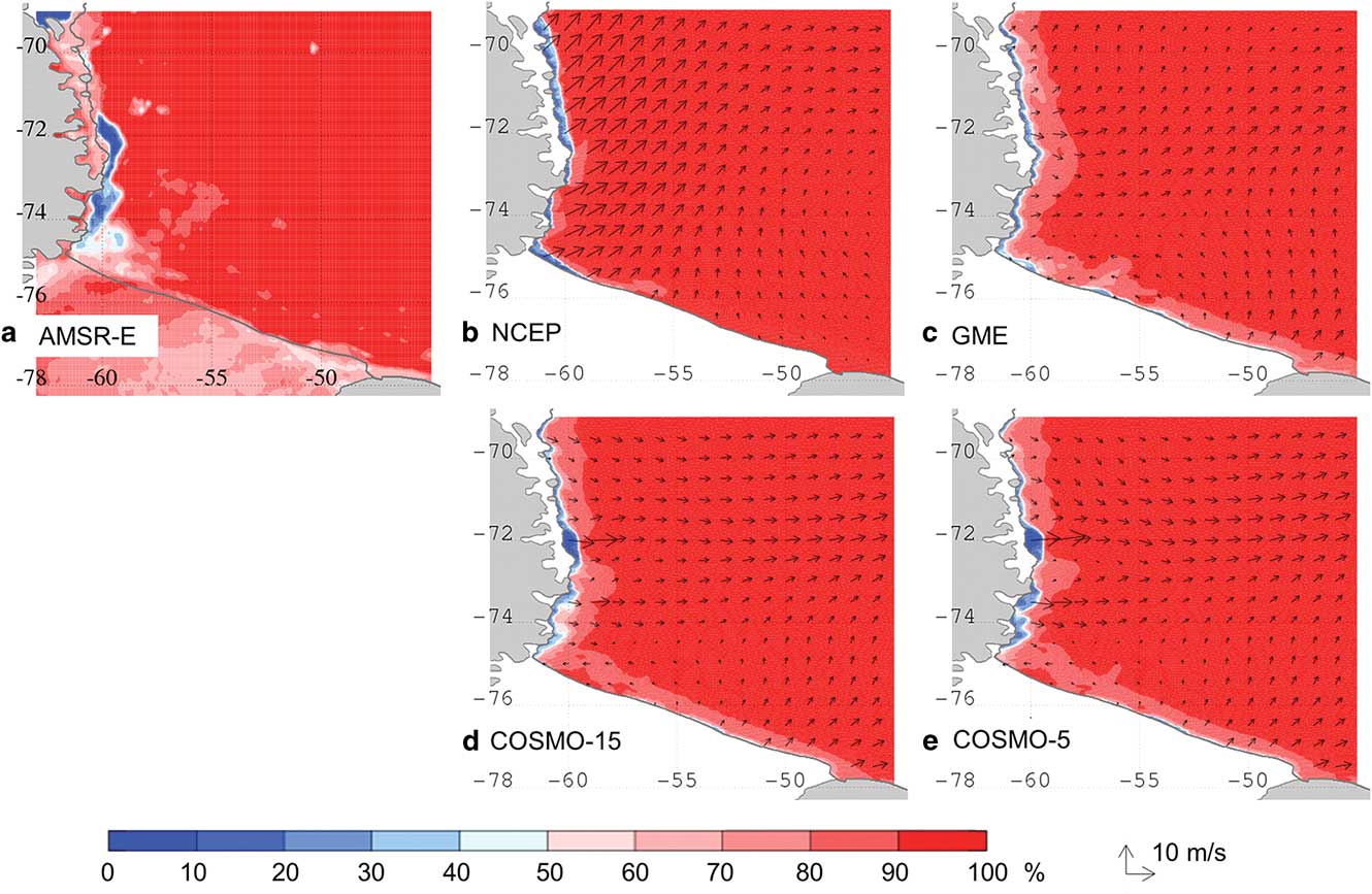
Fig. 7 Sea ice concentration on 29 August 2008. a. AMSR-E satellite data, b. NCEP, c. GME, d. COSMO-15 and e. COSMO-5 simulations. The corresponding wind field is superimposed as black arrows in panels b.–e.
The two simulations with coarser resolution forcing data (NCEP and GME, Fig. 7b–c) feature a belt of reduced sea ice concentration with only few interruptions along the entire western coastline. Both datasets feature a wind field and accordingly a polynya width with little variation along the coastline, although with different characteristics in the respective experiments. Much better agreement with the satellite measurement is achieved by the two simulations with high-resolution COSMO forcings (Fig. 7d–e). Both feature a narrow polynya along the entire western coastline but also capture the strong widening of the polynyas at ≈72°S, ≈73.5°S and ≈74.5°S (slightly more distinct with COSMO-5 than with COSMO-15). This local intensification is also visible in the wind field and is caused by the steering effect of the large valleys facing the coastline. It is clear that the small-scale features of the inland topography have a substantial effect on the formation of coastal polynyas here and that increasing resolution in the atmospheric simulations improves the performance of the sea ice model.
Although locally the results of the experiments can differ substantially, in a basin-scale view of the entire south-western Weddell Sea (Table I) most of these local differences compensate each other, thus mean values are similar between the simulations with different forcing datasets.
High Salinity Shelf Water production and export
Salinity increase
During autumn and winter, the sea ice production exerts a strong influence on the shelf waters by accumulating salt in the water column. Thus, the differences in ice production are propagated to changes in salinity. From April to August, the salinity on the continental shelf increases in all experiments. In general, we find the strongest increase in bottom salinity is found over the shallowest part of the coastline in front of Berkner Island and the eastern part of Ronne Ice Shelf (Fig. 8). In the NCEP run (Fig. 8a–c), the outer part of the Berkner Bank and the Ronne Depression (except in 2008) also feature maxima of bottom salinity increase. With the exception of small areas at the Antarctic Peninsula coastline, the rest of the continental shelf experiences no major salinity increase at the bottom.
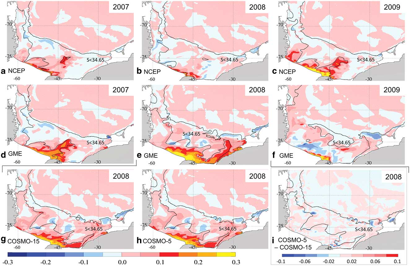
Fig. 8 Increase of bottom salinity maps over April to August. a.–c. NCEP analysis and d.–f. GME analysis for 2007–09. g. & h. COSMO-15 and COSMO-5 forecasts for 2008. i. Difference between COSMO-5 and COSMO-15 forecasts. The solid black line marks the bottom salinity contour of 34.65 at the end of August. In i. the salinity contour of the COSMO-5 data is plotted for orientation. Please note that i. uses a different scale and that
 $$S$$
>34.65 is typical for both High Salinity Shelf Water and Warm Deep Water.
$$S$$
>34.65 is typical for both High Salinity Shelf Water and Warm Deep Water.
This pattern of salinity increase results in water with
 $$S$$
>34.65 (solid black line in Fig. 8) filling the western area from Ronne Depression to Larsen C Ice Shelf. Furthermore, high salinity waters are found between General Belgrano Bank and Berkner Bank (see Fig. 1b for location) and locally in front of the eastern Ronne Ice Shelf and at the northern Berkner Bank (less abundant in 2008). In 2009, additional to the aforementioned regions the entire western part of Berkner Bank features bottom salinities >34.65.
$$S$$
>34.65 (solid black line in Fig. 8) filling the western area from Ronne Depression to Larsen C Ice Shelf. Furthermore, high salinity waters are found between General Belgrano Bank and Berkner Bank (see Fig. 1b for location) and locally in front of the eastern Ronne Ice Shelf and at the northern Berkner Bank (less abundant in 2008). In 2009, additional to the aforementioned regions the entire western part of Berkner Bank features bottom salinities >34.65.
The GME experiment, as seen before in other variables, has more variability in the interannual patterns. In 2007, similarities are seen to the NCEP run; however, the bottom salinity increase over Berkner Bank is much stronger and in the Ronne Depression the change is slightly weaker. Further, there is a substantial increase of the bottom salinity under the southern Brunt polynya and to a lesser degree along the Coats Land coastline. Salinities >34.65 are found in the same areas as in the NCEP run, but also covering the entire western part of Berkner Bank. In 2008, the strong sea ice production along the entire coastline from the Brunt Ice Shelf to the Ronne Ice Shelf in the GME run (Fig. 5e) causes a substantial increase in the bottom salinity on most of the eastern continental shelf. The maxima occur at the Brunt polynyas and along the Coats Land coastline, and high values are observed along the eastern slope of Filchner Trough. The area north of Berkner Island and the eastern part of Ronne Ice Shelf feature exceptionally high bottom salinity increases, and in the west a moderate increase stretching from the Ronne Depression along the western side of General Belgrano Bank are apparent. This causes the salinity to rise over the 34.65-threshold of HSSW in extensive areas of the continental shelf.
In 2009, the bottom salinity changes in the GME run are low in most areas of the shelf. A very high salinity increase is visible at the shallow coastline over Berkner Bank, but it remains restricted to a relatively small area. Most of the continental shelf experiences freshening in 2009. However, the preconditioning the on-shelf waters experienced in 2008 leaves the continental shelf almost entirely covered with water with salinities >34.65. Only east of the Filchner Trough, at the outer shelf between 35°W and 50°W, and over the moraine in front of Larsen C Ice Shelf are there lower salinities at the ocean floor.
The changes in the bottom salinity in the COSMO runs again result in almost identical patterns. As the distribution of the sea ice production already indicates, the COSMO results show a pattern of salinity changes similar to the GME run, but reduced in the eastern parts and enhanced in the Ronne Depression. Especially the strong increase of bottom salinity on the eastern flank of Filchner Trough and at the Brunt polynyas is reduced to much weaker maxima and consequently the eastern part of the shelf features lower values.
In 2008, the COSMO experiments show water with
 $$S$$
>34.65 in very much the same areas as in the GME experiment. Only in the northern part of the Filchner Trough and beneath the southern Brunt polynya the threshold is not reached by the bottom waters in the COSMO simulation to a similar extent. The differences in salinity change between the two COSMO runs are primarily found at the shelf break, where dense water plumes and warm water intrusions occur, and on the shelf close to the 34.65 isoline, where dense water plumes show up at different locations. In all simulations, the signatures of decreasing salinities in Fig. 8 are mostly associated with the relocation of salinity maxima from the previous winter by the ocean currents. Mixing with less saline ambient water contributes to the effect.
$$S$$
>34.65 in very much the same areas as in the GME experiment. Only in the northern part of the Filchner Trough and beneath the southern Brunt polynya the threshold is not reached by the bottom waters in the COSMO simulation to a similar extent. The differences in salinity change between the two COSMO runs are primarily found at the shelf break, where dense water plumes and warm water intrusions occur, and on the shelf close to the 34.65 isoline, where dense water plumes show up at different locations. In all simulations, the signatures of decreasing salinities in Fig. 8 are mostly associated with the relocation of salinity maxima from the previous winter by the ocean currents. Mixing with less saline ambient water contributes to the effect.
High Salinity Shelf Water volume and export
The changes in salinity have a direct influence on the production of HSSW. In 2007 and 2009 the volume increase of HSSW (Fig. 9a) is similar in the NCEP and GME runs; in 2008, however, the HSSW volume develops very differently between the runs. Of the 3 years, the NCEP run features the lowest production of HSSW (2.4·104 km3) in 2008, while the GME run has a maximum production (6.8·104 km3) in the same year. With the initial volume difference from the previous summer season, this results in a difference of 7.1·104 km3 in HSSW volume, most of which (4.5·104 km3) is maintained over the course of the following year.
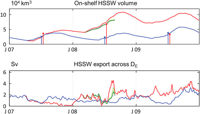
Fig. 9a On-shelf High Salinity Shelf Water (HSSW) volume and seasonal increase (vertical lines). b. HSSW export across DE (Fig. 1b) in the NCEP (blue), GME (red), COSMO-15 (dark green) and COSMO-5 (light green) model simulations for 2007–09.
The large differences in HSSW volume in the first years after the branch-off are still under the influence of a spin-up phase and do not show an equilibrium state in the GME (and COSMO) run. However, we consider the strong tendency toward a larger HSSW volume in the GME run to be persistent. In the COSMO runs, the HSSW volume features a similar behaviour as in the GME run, but the increase is slightly less steep, which is consistent with the smaller ice production in the COSMO simulations.
In the NCEP simulation, the HSSW volume features a seasonal cycle but no substantial differences between the 3 years. In 2008, slightly less HSSW is produced than in the previous year and 2009 features the maximum production. These interannual differences of the NCEP simulation, however, are small compared to the differences between experiments that are predominantly linked with events in 2008.
In 2007, much of the HSSW in the GME run is produced near Berkner Island and the eastern part of Ronne Ice Shelf (Fig. 8d). Therefore, it has to be advected far to the west and north before it leaves the continental shelf. Since on the western part of the shelf, especially over the Ronne Depression, little salt is added to the water column, the export of HSSW in the GME experiment is small in 2007. Although the HSSW volume increases, the export drops to almost zero at the end of the year (Fig. 9b) and causes the HSSW volume to increase even late in the year. Consequently, in autumn 2008, a large volume of preconditioned water is visible on the continental shelf. The HSSW production occurs extensively in the eastern part of the shelf and also in the west over the Ronne Depression (Fig. 8e). The HSSW volume reaches very high levels and covers large areas of the shelf. The export recommences and export rates increase rapidly at the end of July to peak in August with a maximum of 4.6 Sv (Fig. 9b); thereafter, the HSSW export drops again to values ≈2 Sv. In 2009, HSSW export rates increase again.
The HSSW export in the NCEP run features maxima of 2 Sv and minima of 0.5 Sv, alternating in a rugged seasonal cycle, during most of the 3 year period. In spring 2009, however, export maxima of 3.5 Sv are reached. This gives a mean export rate of 1.3 Sv for the NCEP run, while the GME run yields a higher mean export rate of 1.7 Sv. The COSMO experiments during the first half of the experiment feature higher HSSW export rates than the GME run, but in the second half the values stay below the GME results. Unfortunately, the COSMO time series are too short to conclude on the behaviour over longer time scales.
Summary and conclusion
To investigate the impact of differences in the atmospheric forcing data on the extent of coastal polynyas, sea ice production and shelf water properties in the south-western Weddell Sea, simulations of the sea ice–ocean model FESOM were conducted using atmospheric forcing data from the NCEP/NCAR reanalysis, GME, and two configurations of the regional COSMO model. Both GME and NCEP forcing fields and results were compared for three consecutive autumn/winter periods (April to August 2007–09); COSMO output was only available for 2008.
The mean wind field reveals substantial differences between the forcing models. At the coastline of the Antarctic Peninsula, where the NCEP forcing features a wind speed maximum with south-westerly wind directions, the GME data feature weak southerly winds. Further, at the Brunt Ice Shelf the NCEP wind speed has a maximum, while the GME data (except in 2008) features reduced wind speeds. However, in general, GME features the strongest winds of all of the datasets. The centre of the basin-scale rotation of the wind is farther east in the GME data than in the NCEP data and, therefore, south-westerly winds over the basin’s centre are only found in the GME data. The air temperatures feature no blatant differences in their spatial patterns; however, the NCEP data has the coldest mean air temperatures and the COSMO forcings the warmest.
While the NCEP forced simulation tends to underestimate polynya size (with the exception of the Antarctic Peninsula region), the GME experiment seems to overestimate polynya formation (especially on the eastern part of the shelf). The most striking difference between the two coarser datasets is found in front of Filchner Ice Shelf, where the effects of the iceberg A23 prevent a clarifying comparison to satellite data.
Sea ice formation, which is highest in coastal polynyas and, therefore, very dependent on the wind field, is most active in the GME run. The most notable difference to the NCEP run is the strong activity on the eastern part of the continental shelf. Furthermore, in the COSMO runs substantial ice production is visible in the east, but less than in the GME run; the ice formation of the COSMO runs at the westernmost part of Ronne Ice Shelf is higher than in both NCEP and GME runs (since NCEP features exceptionally little polynya activity in 2008). An evaluation of variability shows that most major short-term events are consistently found in all four atmospheric datasets.
The large differences are striking between NCEP and GME forcing for 2008, a year with a pronounced La Niña/positive SOI event. While in the GME run the largest polynyas are formed and consequently ice production is high, the NCEP forcing features the least activity in this year. In both datasets, a strengthened cyclonic flow in the mean wind field can be seen; however, in the GME data it is located to the east and causes strong south-westerly winds over the central open ocean that drive the sea ice north and out of the basin, while in the NCEP forcing the centre of the cyclonic circulation is further west (consistent with the composite analysis of Kwok & Comiso Reference Kwok and Comiso2002) and sea ice drift out of the basin is not supported.
At the Coats Land coastline the differences between the NCEP run, where almost no polynyas are formed, and the GME experiment, where we find large polynyas, are consistently seen in all years. In contrast, differences between the coarse-scale GME data and the high-resolution COSMO datasets are comparatively small. However, the offshore winds at the Coats Land coastline in the COSMO data are consistently smaller than the offshore winds in the GME data. At a basin-scale consideration, however, most of the local differences compensate each other and the results for sea ice formation from the different atmospheric forcings agree well.
For the salinity, the quantity and distribution of sea ice formation are both important. The area in front of Berkner Island and the western Ronne Ice Shelf, due to its shallow water column, always features the highest increases in salinity. In the NCEP run, the maxima of salinity increases are usually in the Ronne Depression and the outer part of Berkner Bank, while in the GME run the pattern changes between years. In 2008, a very low salinity increase was seen in the NCEP run, while the GME run (responding to increased sea ice formation) features a strong salinity increase, most prominently in the eastern areas between Brunt Ice Shelf and Berkner Bank but also along the Ronne Ice Shelf front and moderately in Ronne Depression. Compared to the GME pattern, the COSMO runs feature lower salinity increases in the eastern regions, but an amplified salinity increase in the area of the Ronne Depression.
In consequence, the HSSW volume increases strongly in 2008 in the GME experiment, but only slightly in the NCEP simulation, while in 2007 and 2009 the increase in HSSW volume is similar in both cases. However, the strong increase of HSSW volume in the GME experiment in 2008 affects the total HSSW volume present on the shelf and the salinity in the subsequent years. The export of HSSW is higher with GME forcing and its strong variations differ from the export found in the NCEP simulation. The mean export of HSSW for the 3 year period is 1.3 Sv in the NCEP simulation and 1.7 Sv in the GME experiment.
In a slightly more general view, several interesting findings arise from this study. Evaluating the differences between the various forcing fields and simulations, it turns out that the differences in the far field, namely the locations of the centre of the cyclonic pattern that dominates the large-scale wind field (and thus the sea ice drift) in the Weddell Sea, are more important for the formation of coastal polynyas than the local wind field. Despite strong offshore winds in the Ronne region in the NCEP experiment, polynya area in this simulation is not particularly high, because the far field wind pushes the sea ice into the south-west corner of the Weddell Sea (instead of driving it northward into the central Weddell Sea, as is the case in the GME and COSMO runs). As a consequence, the regional sea ice production in the Ronne area in the NCEP experiment is comparatively small.
The importance of the large-scale wind pattern is also illustrated by the effect of the different signatures of the La Niña event in 2008. Both show an enhanced cyclonic circulation (consistent with the pattern suggested by Kwok & Comiso Reference Kwok and Comiso2002), but due to the different locations of the centre of this cyclone, the effect on sea ice formation rates is very different with increased sea ice formation with GME forcing, and reduced sea ice formation in the NCEP case. Offshore winds that potentially drive the formation of coastal polynyas are sufficiently present in all simulations, but large polynyas only occur if the large-scale ice drift field allows for an easy export of newly formed ice.
While it seems reasonable to expect a consistent, monotonous change in properties from the coarse-scale NCEP dataset via the higher-resolution GME data to the high-resolution COSMO results, this is really not the case. Instead, the NCEP and GME results mark the extremes of the range for wind speed, polynya area and sea ice formation / salt release in many cases; with GME always representing the maximum. The COSMO results are consistently closer to those of the GME run than to those of the NCEP run, but generally do not exceed the maximum given by the GME results. The COSMO model was forced with lateral boundary conditions from GME; therefore, it is not surprising to find COSMO results close to the GME fields. However, it is surprising that compared to the GME results the COSMO results are always towards the lower end of the range; which leads to the conclusion that many of the relevant processes discussed here are overestimated in the GME simulations. In contrast to NCEP, the resolution of GME is sufficient to simulate modifications of the wind field by Berkner Island, which results in large differences in ice production at the Filchner Ice Shelf front.
Finally, high-resolution atmospheric forcing, as represented by the COSMO results here, has been shown to make a difference mainly in mountainous areas, where katabatic winds occur and air flow is strongly guided by surface topography. In these regions, namely close to Coats Land and along the Antarctic Peninsula, the use of a high-resolution wind field results in a substantial improvement of the representation of polynya formation in a sea ice-ocean model.
The change from 15 km to 5 km resolution in the atmosphere model seems to lead to further improvement. However, the changes are small when averaged over a winter period and very local, thus for many purposes other than kilometre-scale studies the use of a 15 km atmospheric dataset may well be appropriate and certainly help to reduce the computational burden. Furthermore, while insufficient for studies of regional effects (e.g. the circulation under the Ronne-Filchner Ice Shelf), a coarse-scale reanalysis dataset with a well-validated large-scale wind pattern still appears to be an appropriate choice for basin-scale mean values.
Acknowledgements
This study was supported by Deutsche Forschungsgemeinschaft in the framework of the priority programme SPP 1158 ‘Antarctic Research with comparative investigations in Arctic ice areas’ under grant numbers Ti 296/5 and He 2740/10. The authors wish to thank DWD for providing the COSMO model and GME data and the DKRZ (Hamburg) for providing computing time. The NCEP/NCAR reanalysis data was obtained from NOAA Climate Diagnostics Center, Boulder, CO, USA via the website http://www.cdc.noaa.gov. The AMSR-E data was obtained from Zentrum für Marine und Atmosphärische Wissenschaften, Hamburg, Germany via the website ftp://ftpprojects.zmav.de/seaice/. We thank Alexandra Weiss and an anonymous reviewer for their helpful comments.
Author contribution
Verena Haid: sea ice–ocean simulation, visualization of results, writing of manuscript. Ralph Timmermann: support of sea ice–ocean simulation, substantial support of manuscript. Lars Ebner: atmosphere model simulations, support of manuscript. Günther Heinemann: support of atmosphere model simulations and manuscript.


