2. Retail Prices

2.1 The most recent series used for the Retail Prices Index is the one called just that, RPI, and not RPIX, CPI, HPI or any of the other alternative series produced for the UK in recent years. As before, we denote the RPI index at time t as Q(t), and we calculate the “force” of inflation over the year t−1 to t, denoted I(t), as I(t) = lnQ(t) – lnQ(t−1), so that Q(t) = Q(t−1).expI(t). In Figure 2.1 we show the values of I(t) from 1900 to 2009.

Figure 2.1 Annual force of inflation, I(t), 1900–2009

2.2 One can observe that in the 15 years or so up to the most recent year the value of I(t) had been much more stable than in many earlier periods, having settled down to a range of about 0.01 to 0.04 since it reduced after the instability of the 1970s and 1980s. But for the year ending June 2009 the value of I(t) was negative, for the first time since 1959, and by a larger amount negative than in any year since 1933. If the long period of stability had continued, it would suggest that a different model, or at least a model with different parameters, might be more appropriate. The return to negative inflation indicates that it might be very difficult at this point to be at all sure. But first we investigate how the 1995 model has fared since that date.

2.3 The original model for I(t) was:

that is QZ(t) is assumed to be a series of independent, identically distributed, unit normal variates, i.e. they have zero mean and unit standard deviation.

2.4 The values of the parameters suggested in 1995, based on the experience from 1923 to 1994, were: QMU = 0.047; QA = 0.58; QSD = 0.0425. In 1995 the experience from 1982 to 1994 was investigated in two ways, first by looking at the residuals, the difference between the ‘forecast’ and the actual values year by year, the observed QEs, or their ‘standardised’ versions, the QZs; and secondly by looking at the cumulative result, the logarithm of the RPI, and comparing it with the values that would have been forecast in 1982. We do the same this time, using the 1995 parameters and starting the forecasts in 1994. The methodology is described in Appendix E of Wilkie (Reference Wilkie1995).

2.5 According to the model, the residuals, the QEs, are distributed N(0, QSD ²), i.e. normally with zero mean and variance QSD ²; it is convenient first to divide each QE by QSD to give QZs; these are assumed to be distributed N(0,1). The sum of n such QZs is distributed N(0, n ²), and the sum of the squares of n such QZs is distributed as χ_n ².

2.6 From 1995 to 2009 we have 15 new values. Table 2.1 shows, for each year, the observed value I(t), the expected value conditional on the relevant information up to year (t−1), E[I(t) |_{t −1}], the observed residual QE(t) = I(t) – E[I(t)|_{t −1}], and the standardised residual QZ(t) = QE(t)/QSD. The notation _t just means the ‘facts’ or the relevant information as known at time t, and is technically a statistical “filtration”.

Table 2.1 Comparison of actual and expected values of I(t), 1995–2009

2.7 We can compare the sum of the 15 values of QZ, which is −3.70, with the expected value, zero, and with the standard deviation √15 = 3.87. It is within one standard deviation away from its expected value. We can also compare the sum of the 15 values of QZ ², which is 3.27 with a χ ₁₅² distribution; the probability of a value of χ ² as great or greater is 0.9993, which suggests that this value of χ ² is exceptionally low. The biggest (absolute) value of QZ is 1.45. The value of QSD looks as if it were much too high, in comparison with the experience of the last 15 years. One might think that this reflected a change in “regime” (as indeed it did, in respect of the Bank of England's monetary policy) and hence that a change in the model, or at least in the parameter values, might be appropriate. But the big jumps in inflation, negative in June 2009, and above 5% in June 2010 suggest that a period of greater instability might be in prospect.

2.8 We can now consider the forecast values of ln Q(t), conditional on the information as at 1994. It is easier to work with the change in the logarithm, i.e. QF(t) = ln Q(t) – ln Q(1994), which is just the cumulative sum of the values of I given in Table 2.1. Using the formulae for the expected values and variances of the forecast log changes, which were set out in Appendix E.2 of the 1995 paper, we get the results shown in Table 2.2. This shows the value of QF(t) for each year, its expected value conditional on the relevant information up to 1994 E[QF(t)|₁₉₉₄], the observed deviation QF(t) – E[QF(t)|₁₉₉₄], the standard deviation of QF(t)|₁₉₉₄, and the standardised residual, the observed deviation divided by the corresponding standard deviation.

Table 2.2 Comparison of actual and expected values of QF(t), 1995–2009 all conditional on ₁₉₉₄.

2.9 The successive values of ln Q(t) are not independent, and the results represent only one experience for 15 years, not 15 independent experiences for 1, 2, …, 15 years. The deviations between the values of ln Q(t) and the forecast values are all negative, indicating that the forecasts based on the 1994 value were too high. This could indicate that the value of the mean estimated in 1995, QMU, was perhaps too high. All the values of ln Q(t) are within one standard deviation of their forecast values. Again, one might think that the ‘expanding funnel of doubt’ has been too wide over this period, i.e. that the value of QSD estimated in 1995 was too high.

2.10 We now re-estimate the parameters for the whole period, 1923–2009. In Table 2.3 we compare these with those that were estimated in 1995. We also show some statistics from both periods: first, the first autocorrelation coefficient of the residuals, the values of QZ(t), denoted r(QZ)₁; then the first autocorrelation coefficient of the squares of the residuals, the values of QZ(t)², denoted r(QZ ²)₁; next the skewness and kurtosis coefficients of the residuals, denoted √β ₁ and β ₂; finally the Jarque-Bera χ ² statistic, equal to the sum of the squares of the skewness and kurtosis coefficients, in each case divided by the squares of their standard errors, together with the probability of such a large value of χ ² being observed. Further details of these statistical tests are given in Wilkie (Reference Wilkie1995), Appendix C.

Table 2.3 Estimates of parameters and standard errors of AR(1) models for inflation, and relevant statistics, over different periods.

2.11 It can be observed that the values of the parameters do not change by much, though the values of QMU and QSD are reduced a little, being influenced by the several recent years of low and stable inflation. The skewness and kurtosis coefficients are increased, not because of any new large outlying values, but because the previous outlying values are divided by a smaller value of QSD. The autocorrelation coefficients, r(QZ)₁, are very low, demonstrating that the residuals have no first order autocorrelation, as one would expect; the autocorrelation coefficients of the squared residuals, r(QZ ²)_1, are a little larger, though far from significant. We do, however, investigate a heteroscedastic (ARCH) model for inflation, in Section 9.

2.12 Possible rounded values for practical use, based on the past experience, might now be:

However, the recent experience suggests that a lower mean value, such as QMU = 0.025, might be more appropriate for the future. We would not, however, recommend reducing the standard deviation, because, in the long run, the path of inflation may be very uncertain. We shall discuss the possibility of using short-term adjustments to the parameters, in the form of a “select period”, in a later article.

2.13 It is clear from the high values of the skewness and kurtosis coefficients that the residuals are far from being exactly normally distributed. We show in Section 9 that an ARCH model makes little difference to this. We shall discuss models for the distribution of residuals also in a later article.

2.14 It has been suggested (e.g. Huber, Reference Huber1997) that, when parameters are estimated over different periods, very different values may be obtained, indicating that the values of the parameters are not stable. We investigate this. Rather than calculate the parameter values over every possible subset of dates, we use only two subsets, those periods starting in 1923, and those periods ending in 2009. When the number of observations is small, less than 10 in this case, we omit the calculations. We display the results in a series of graphs, in Figures 2.2, 2.3 and 2.4, for QMU, QA and QSD respectively. These and subsequent graphs for other parameters all have the same format, which we now explain.

Figure 2.2 Estimates for parameter QMU for periods starting in 1923 and periods ending in 2009, with 95% confidence intervals (The meaning of the lines is described in ¶2.15 and ¶2.16)

Figure 2.3 Estimates for parameter QA for periods starting in 1923 and periods ending in 2009, with 95% confidence intervals (The meaning of the lines is described in ¶2.15 and ¶2.16)

Figure 2.4 Estimates for parameter QSD for periods starting in 1923 and periods ending in 2009, with 95% confidence intervals (The meaning of the lines is described in ¶2.15 and ¶2.16)

2.15 We explain the graphs by using Figure 2.2, for QMU, as an example. The heavy line shows the estimated values of QMU for periods starting in 1923 and ending in the given year. It begins with the period ending in 1932, for which there are 10 years of data from which to estimate the parameters. Over this period we can see that the estimated value of QMU is negative, at −0.0192. As the period increases the value increases, reaching a peak at 0.0503 for the period ending in 1980. Thereafter it drifts slightly down, ending in 2009 at 0.0429, as shown in Table 2.3.

2.16 The thinner continuous line in the graph shows the estimated values of QMU for periods ending in 2009. This line commences in 1923 at the value 0.0429, being the value for the whole period 1923–2009. The line rises gently as the earlier years of negative or low inflation are omitted, and reaches a peak at 0.0597 in 1968. For the most recent years it declines quite sharply, ending at 0.0261 for 2000, the last year for which we have 10 years data ending in 2009. The dotted lines on either side of the thinner continuous line show approximate 95% confidence intervals for the corresponding value; the dot and dash lines on either side of the heavy line do the same. These are based on an assumption that the parameter value is distributed normally, and are calculated as the estimated value plus or minus 1.96 times the calculated standard error.

2.17 It can be seen that the estimated values of QMU are fairly far apart in the earlier years and cross over in 1977. However, the confidence intervals overlap for all years from 1940 onwards. Further a value of 0.030 lies within both confidence intervals for QMU from 1949 onwards. As the periods shorten one would expect the confidence intervals to widen, being based on fewer observations. In fact they do the opposite. In the most recent periods the confidence intervals are quite narrow, being based on a period when the rate of inflation has been relatively low and very stable. This is most obviously seen from the very low values for QSD in the recent periods seen in Figure 2.4.

2.18 Figure 2.3 shows the same features for QA, using the same conventions. Coming forward from 1923, we see rather low values, starting at around 0.2, rising to a plateau of about 0.4 and then to another plateau of about 0.6. Then reducing the periods, but keeping the end point at 2009, the 0.6 value is apparent for a long period, but in the most recent years the value has dropped, to well below zero. The confidence intervals overlap for almost all the periods shown, but are comparatively wide, especially for the most recent years. When inflation is very stable, and has a low variability, any autoregressive tendency that might be observed when rates are much higher cannot be identified.

2.19 In Figure 2.4 one can see the graphs for QSD. The most obvious feature is how much lower the values have been in recent years, and how narrow the confidence interval has also been. This almost suggests that a “regime switching” model might reflect the facts rather better than a model with fixed parameters. But we discuss this further when considering an ARCH model in Section 9.

2.20 We have noted that the kurtosis of the residuals of the fitted model is large, indicating that the residuals are fatter-tailed than they would be if they came from a normal distribution. One possibility would be to use a different theoretical distribution, which was fatter-tailed than the normal one. If we were to do this, the standard errors for the estimates of the values of the parameter would very probably be larger, perhaps much larger, than we have shown in Table 2.3. Further, the confidence intervals shown in the partial-period graphs would be wider. In any case, the standard errors shown in Table 2.3 are not small, and would give 95% confidence intervals for the value of QMU of about 0.02 to 0.06 (i.e. about 2% to 6% mean inflation), for the value of QA of about 0.43 to 0.73, for the value of QSD of about 0.034 to 0.046. If we wish to simulate the values of Q(t) over a number of future years we would be well-advised both to allow for the quite large uncertainty in the values of the parameters, and to use a fatter-tailed distribution than the normal for the future random innovations. These observations apply to all our series, to a greater or lesser extent. However, further discussion of these points is deferred to later articles in this series.

3. Wages

3.1 For wages we use a series of indices, ending with the index for Monthly Earnings, All Employees, not seasonally adjusted. We denote the wages index at time t as W(t), and the force of wage inflation over the year t−1 to t as J(t), calculated as J(t) = lnW(t) – lnW(t−1), so that W(t) = W(t−1).exp J(t). In Figure 3.1 we show the values of Q(t) and W(t) from 1900 to 2009. We see that, after a rise from 1915 to 1920 and a subsequent fall, both series have risen on the same lines, but moving apart a little.

Figure 3.1 Retail prices index, Q(t), and Wages index, W(t), 1900–2009

3.2 In Figure 3.2 we show the logarithm of “real wages”, that is ln{W(t)/Q(t)}, and also a line of constant growth from 1923 to 2009, at a force of 0.0146 per year. We see how, since 1923, the difference between the two series, lnW(t) and lnQ(t), has tracked the line quite closely. This might suggest that the two series are co-integrated. We intend to investigate this idea in a later article in this series.

Figure 3.2 Logarithm of real wages, ln{W(t)/Q(t)} 1900–1923, and constant growth line based on 1923 to 2009

3.3 In Figure 3.3 we show the values of I(t) and J(t). These too have been quite similar over the period, especially since 1923. Since 1994 the wage inflation has, like price inflation, been at a much lower, and more stable, level than in previous years.

Figure 3.3 Price inflation, I(t), and Wage inflation, J(t), 1900–2009

3.4 The model for J(t) suggested in 1995 can be written as:

3.5 Two sets of values of the parameters were suggested in 1995, based on the experience from 1923 to 1994. In both the value of WA was taken as zero. In one (Model W1) the values of the other parameters were: WW1 = 0.60; WW2 = 027; WMU = 0.021; WSD = 0.0233. In the other (Model W2): WW1 = 0.69; WW2 = 1−WW1 = 031; WMU = 0.016; WSD = 0.0244. We investigate the experience from 1994 to 2009 in the same two ways as for I(t) and Q(t). In the first we look at the forecast residuals for year t conditional on knowledge both of _{t –1} and of I(t), i.e. assuming that we know the rate of price inflation in year t. In the second we look at the cumulative result and compare it with the values that would have been forecast in 1994.

3.6 From 1995 to 2009 we have 15 new values. Table 3.1 shows, for each year, the observed value J(t), and for each model the expected value conditional on the relevant information including the current inflation, E[J(t)|_{t− 1} & I(t)], the observed residual WE(t) = J(t) – E[J(t)|_{t− 1} & I(t)], and the standardised residual WZ(t) = WE(t)/WSD. We can see that the standardised residuals are very low, only recently getting bigger (absolutely) than 1.0, and with a total and a value of the sum of squares that are all very low. We might assume that the value of WSD found in 1995 has been too big, compared with the experience of the last 15 years.

Table 3.1 Comparison of actual and expected values of J(t), 1995–2009, conditional on _{t −1} and I(t), using Models W1 and W2.

3.7 In Tables 3.2a and 3.2b we see the same, all based only on the data as at 1994, ₁₉₉₄, and using models W1 and W2 respectively. The standard deviations allow for the uncertainty of forecast inflation, as well as that of real wages, and the deviations are all negative, since inflation has been lower than the expected in 1994. However, all the deviations except the last for W1 are within one standard deviation, and that for W1 for 2009 is only −1.02.

Table 3.2a Comparison of actual and expected values of WF(t), 1995–2009, using Model W1, all conditional on ₁₉₉₄.

Table 3.2b Comparison of actual and expected values of WF(t), 1995–2009, using Model W2, all conditional on _1994.

3.8 We now re-estimate the parameters for the whole period, 1923–2009. We do this for four different models, with WA free or set to zero, and with WW2 free or set to 1−WW1. In Tables 3.3a and 3.3b we compare these with those that were estimated in 1995, in each case along with the same statistics as shown for inflation in Table 2.3.

Table 3.3a Estimates of parameters and standard errors of two models for wages, with WA = 0, and relevant statistics, over different periods.

Table 3.3b Estimates of parameters and standard errors of two models for wages, with WA free, and relevant statistics, over different periods.

3.9 We can observe that, as in 1995, the addition of the WA term improves the log likelihood by very little, and in one of the cases it worsens the fit, and further that the value of WA is not significantly different from zero. So the WA term can be omitted. In 1995 there was not a very big difference between the model with WW2 free and the one with WW2 = 1−WW1. The same is true on this occasion, though the fit on both occasions is not so good. There is therefore good reason to prefer the model with WW2 free, even though this does not give a “unit gain” from inflation to wages.

3.10 Possible rounded values for practical use, based on the past experience, might now be:

or alternatively

These are almost the same as those suggested in 1995. Both omit the WA term. In the first model, when WW2 is free, the kurtosis coefficient is not exceptionally large, and the Jarque-Bera statistic is acceptable. In the other model, the high value of the kurtosis coefficient indicates that the residuals are not close to being normally distributed, though they are less far away than the inflation residuals, partly because the values of inflation are already included in the formula, and the wage residuals represent variation over and above the variation due to inflation.

3.11 We now show, as for inflation, graphs of the estimated values of the parameters over various subperiods, those starting in 1923 and those ending in 2009. We do this only for our preferred model, with WW2 free and WA = 0, and show graphs for WW1, WW2, WMU and WSD in Figures 3.4 to 3.7 respectively.

Figure 3.4 Estimates for parameter WW1 for periods starting in 1923 and periods ending in 2009, with 95% confidence intervals (The meaning of the lines is described in ¶2.15 and ¶2.16)

Figure 3.5 Estimates for parameter WW2 for periods starting in 1923 and periods ending in 2009, with 95% confidence intervals (The meaning of the lines is described in ¶2.15 and ¶2.16)

Figure 3.6 Estimates for parameter WMU for periods starting in 1923 and periods ending in 2009, with 95% confidence intervals (The meaning of the lines is described in ¶2.15 and ¶2.16)

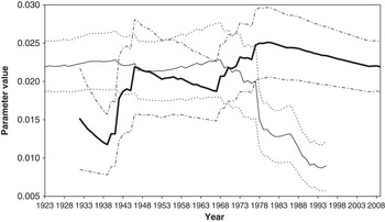
Figure 3.7 Estimates for parameter WSD for periods starting in 1923 and periods ending in 2009, with 95% confidence intervals (The meaning of the lines is described in ¶2.15 and ¶2.16)

3.12 In Figure 3.4 we can see that the estimates for WW1 for periods starting in 1923, the solid black line, are reasonably constant, whereas those for periods ending in 2009, the thinner continuous line, drop quite sharply in the most recent years. The same is true for the estimates for WW2, which is even more stable in the earlier years. The considerable reduction in these two factors in recent years is consistent with rather stable increases in both prices and wages, which gives the impression that the two series have little connection, even though the connection is very strong when inflation is high.

3.13 The charts for WMU are reasonably stable too, except that the estimated value has risen in the most recent years. This compensates for the reduction in WW1 and WW2; if wage increases are not dependent on inflation, from which they would obtain roughly the mean increase in prices, they must have their own, larger, mean increase.

3.14 The charts for WSD, however, are much less stable, and show much reduced values for the shorter recent periods. This is consistent with the much more stable pattern of wage increases in recent years, but it would be premature at this point to assume that this stability will continue indefinitely.

4. Share Dividend Yields

4.1 The share dividend yield is based on a number of indices, since 1962 on the FTSE-Actuaries All-Share Index. The yield for most of the period has been based on the gross dividend index, i.e. gross of income tax, which non-tax paying investors, such as UK pension funds, could reclaim. However, during the 1990s this was confused by the introduction of Foreign Income Dividends, which carried a non-reclaimable tax credit, and then in 1998 the tax credit was reduced to 10% of the gross amount, and in almost all circumstances this tax credit could not be reclaimed. Thus companies started declaring “actual dividends”, to which a tax credit of one-ninth was added, and the published dividend yield was based on actual dividends. In order to keep continuity with the past, we have grossed up the actual yields by one-ninth since 1999. But if one is looking to the future, other adjustments should be made, which we describe in ¶4.8.

4.2 The dividend yield is shown in Figure 4.1, at annual intervals, from 1919 to 2009. We can see that it reached very low levels during the bubble of the late 1990s, but has risen recently and is now above its long run mid-point of around 4%. We should observe, however, that the published dividend yield is based, in general, on recent past dividends (i.e. is a “historic” yield), rather than on prospective future dividends. The rise in yields in 2008 and 2009 was mainly because of a fall in share prices, though the dividend index did rise considerably in the year to June 2008, falling again in the year to June 2009. The fact that share prices do to some extent anticipate changes in dividends is reflected in the YE(t–1) term in the model for dividends.

Figure 4.1 Share dividend yield, Y(t), %, 1919–2009

4.3 The original model for Y(t) was:

4.4 The values of the parameters suggested in 1995, based on the experience from 1923 to 1994, were: YW = 1.8; YMU = 0.0375; YA = 0.55; YSD = 0.155. We investigate the forecast, using these parameter values, in Table 4.1 and Table 4.2. We assume in Table 4.1, which shows the one-step ahead forecasts, that we know the value of I(t) before we forecast Y(t). There were several years on either side of 2000 when the dividend yield was very low, so there are rather large negative values of YZ(t), but in the last two years the reverse has occurred, with relatively large positive values. Nevertheless, the sum of the values of YZ(t) is comfortably within a confidence region, as is the sum of squares, which has a p-value of 0.25.

Table 4.1 Comparison of actual and expected values of ln Y(t), 1995–2009, conditional on _{t −1} and I(t).

Table 4.2 Comparison of actual and expected values of lnY(t), 1995–2009, all conditional on _1994.

4.5 In Table 4.2 we show the forecast values of lnY(t), conditional on the information as at 1994. Most of the deviations are negative, though the most recent ones are positive, but in 1999 to 2001 the values of the standardised deviations were below −2.0, showing that the “bubble” of that period was rather outside what might have been forecast in 1994. But overall the results are satisfactory.

4.6 In Table 4.3 we compare the parameters estimated for the whole period, 1923–2009, with those that were estimated in 1995, along with the usual statistics.

Table 4.3 Estimates of parameters and standard errors of models for dividend yield, and relevant statistics, over different periods

4.7 It can be observed that the values of the YMU and YSD are almost unchanged, while YW is reduced and YA is increased. The skewness and kurtosis coefficients are quite close to zero and 3 respectively, and the Jarque-Bera test is quite satisfactory, although higher than previously, but still indicating that the residuals can be assumed to be fairly close to being normal. The autocorrelation coefficients are reasonably low, showing that we do not need to look for a heteroscedastic model for this series.

4.8 Possible rounded values for practical use, based on the past experience, might now be:

However, because of the change in the way in which dividends are now taxed, as described in ¶4.1, it may be appropriate for the future to use the “actual yield” basis, in which case the value of YMU should be reduced by 10% to give a value of 0.03375 or 3.375%.

4.9 The values of the skewness and kurtosis coefficients, and of the Jarque-Bera statistic, show that the residuals are close to being normally distributed. The extremes that exist in the original data are taken care of by the influence of inflation.

4.10 We show, as before, graphs of the estimated values of the parameters over various subperiods, those starting in 1923 and those ending in 2009. We show graphs for YW, YMU, YA and YSD in Figures 4.2 to 4.5 respectively.

Figure 4.2 Estimates for parameter YW for periods starting in 1923 and periods ending in 2009, with 95% confidence intervals (The meaning of the lines is described in ¶2.15 and ¶2.16)

Figure 4.3 Estimates for parameter YMU for periods starting in 1923 and periods ending in 2009, with 95% confidence intervals (The meaning of the lines is described in ¶2.15 and ¶2.16)

Figure 4.4 Estimates for parameter YA for periods starting in 1923 and periods ending in 2009, with 95% confidence intervals (The meaning of the lines is described in ¶2.15 and ¶2.16)

Figure 4.5 Estimates for parameter YSD for periods starting in 1923 and periods ending in 2009, with 95% confidence intervals (The meaning of the lines is described in ¶2.15 and ¶2.16)

4.11 In Figure 4.2 we see that the influence of inflation on dividend yields, expressed through YW, has been fairly steady over the longer periods, which include the 1940s to the 1970s. But over the early and later shorter periods, the influence has been small or negative, and the confidence intervals are very wide.

4.12 In Figure 4.3 we see that the estimates of YMU are very stable, though the confidence intervals widen when there are fewer observations. The values of YA and YSD are also fairly stable, except in the short early periods.

5. Share Dividends

5.1 Share dividends and share prices come from the same source as the share dividend yield and are subject to the same comments about tax as the dividend yield. The published figures are for share prices, P(t), and dividend yields, Y(t), and the dividend index, D(t), is first calculated as D(t) = P(t) × Y(t)/100, and is then rescaled as convenient. The dividend index is plotted in Figure 5.1, along with Share prices and the Retail prices and Wages indices. We can see that all four series tend to move broadly together, which indicates possible co-integration. We take account of the co-integration of share dividends and share prices by explicitly modelling their ratio, Y(t).

Figure 5.1 Share dividends, D(t), share prices, P(t), 1919–2009 also Retail prices, Q(t), and Wages, W(t), 1900–2009

5.2 We calculate the “force” of increment in the dividend index t−1 to t, denoted K(t), as K(t) = lnD(t) – lnD(t−1), so that D(t) = D(t−1).expK(t). In Figure 5.2, we show the values of D(t) from 1920 to 2009, along with the rate of inflation, I(t).

Figure 5.2 Increase in share dividends, K(t), 1919–2009 and Inflation, I(t), 1900–2009

5.3 The model for D(t) proposed in 1984 and used again in 1995 was:

In this the function DM(t) is an exponentially weighted moving average of inflation up to time t. DI(t) takes a proportion of this and a proportion of the latest rate of inflation. DX is constrained to equal 1−DW, so that there is ‘unit gain’ from inflation to dividends. K(t) is also influenced by the residuals from the previous year of dividend yields and the dividend index itself.

5.4 The values of the parameters suggested in 1995, based on the experience from 1923 to 1994, were: DW = 0.58; DD = 0.13; DX = 1−DW = 0.42; DMU = 0.016; DY = −0.175; DB = 0.57; DSD = 0.07. We investigate the performance against this model since 1994 in Table 5.1, on a year-to-year basis, and Table 5.2 based on starting in 1994. We see that the model did very well, with fairly low values of DZ(t), mixed in sign, until 2008. In that year there was an unexpectedly big rise in dividends (“unexpected” in the sense of being rather outside that expected by the model on the assumption of a normal distribution of innovations), of about 22%, giving a DZ(t) of +2.54, followed in 2009 by an even more unexpected 16% drop, with a DZ(t) of −3.48. The sum of the squares of DZ is 26.83, giving a p-value of 0.03, which is not too extreme.

Table 5.1 Comparison of actual and expected values of K(t), 1995–2009, conditional on _{t −1} and I(t) and Y(t).

Table 5.2 Comparison of actual and expected values of DF(t), 1995–2009, all conditional on ₁₉₉₄.

5.5 In Table 5.2 we show the forecasts since 1994, based on conditions at that date, and showing the forecasts of the cumulative change since that date in lnD(t), denoted DF(t) and calculated as lnD(t)−lnD(1994). From 1999 onwards the deviations are all negative, but are hardly outside one standard deviation. The main reason for the negative deviations is that inflation has been much lower than would have been expected on the 1995 model.

5.6 In Table 5.3 we compare the parameters estimated for the whole period, 1923–2009, with those that were estimated in 1995, along with the usual statistics. They are all different, but not excessively so, and the changes are well within a reasonable confidence interval.

Table 5.3 Estimates of parameters and standard errors of models for dividends, and relevant statistics, over different periods.

5.7 Possible rounded values for practical use, based on the past experience, might now be:

5.8 The residuals are only marginally different from being normally distributed.

5.9 We show, as before, graphs of the estimated values of the parameters over various subperiods, those starting in 1923 and those ending in 2009. We show graphs for DW, DD, DMU, DY, DB and DSD in Figures 5.3 to 5.8 respectively, but not for all subperiods.

Figure 5.3 Estimates for parameter DW for periods starting in 1923 and periods ending in 2009, with 95% confidence intervals (The meaning of the lines is described in ¶2.15 and ¶2.16)

Figure 5.4 Estimates for parameter DD for periods starting in 1923 and periods ending in 2009, with 95% confidence intervals (The meaning of the lines is described in ¶2.15 and ¶2.16)

Figure 5.5 Estimates for parameter DMU for periods starting in 1923 and periods ending in 2009, with 95% confidence intervals (The meaning of the lines is described in ¶2.15 and ¶2.16)

Figure 5.6 Estimates for parameter DY for periods starting in 1923 and periods ending in 2009, with 95% confidence intervals (The meaning of the lines is described in ¶2.15 and ¶2.16)

Figure 5.7 Estimates for parameter DB for periods starting in 1923 and periods ending in 2009, with 95% confidence intervals (The meaning of the lines is described in ¶2.15 and ¶2.16)

Figure 5.8 Estimates for parameter DSD for periods starting in 1923 and periods ending in 2009, with 95% confidence intervals (The meaning of the lines is described in ¶2.15 and ¶2.16)

5.10 The number of parameters is larger than for other models, and their instability is very great. We therefore omit subperiods of less than 20 years, at both the start and the end of the period. Then for many periods, including most periods starting in or after 1971, the maximum likelihood estimate of the value of DW is negative, and sometimes also the estimated value of DD is greater than 1, which would imply that the further back we look at inflation, the greater the effect on dividend increases. This makes no sense, so we omit the values of DW and DD for these periods. The values of the other parameters, however, seem quite sensible, and we leave them in. Sometimes DW is greater than 1, which implies that past inflation has a positive effect, but current inflation a negative one; this is not entirely implausible.

5.11 Where we show it, the value of DD is stable, as is the value of DMU, which is generally greater than zero, but not by much. The values of DY seem to have been increasing, and those of DB and DSD decreasing.

6. Long Term Bond Yields

6.1 For long-term bond yields, C(t), the earlier values are the yield on Consols, later the yield on the FTSE-Actuaries BGS Indices irredeemables yield, which is now purely the yield on War Stock (War Loan). These indices have the advantages of being yields on near-irredeemable stocks (they could be redeemed if market yields fall enough), so are independent of coupon or redemption date; also there is a very long past history. However, the stocks have had special features, and are now relatively small, so they are not fully representative of the long end of the market. But there is no other index that is any better.

6.2 For short-term bond yields, B(t), discussed further in Section 7, Bank Rate or Bank Base Rate has been used. This is not suitable for measuring short-term movements of yields, because it changes only occasionally, so is a step function. But this is not a problem when it is sampled at annual intervals, and it too has a very long past history.

6.3 For index-linked yields, R(t), discussed further in Section 8, the yield from the FTSE-Actuaries BGS indices on index-linked stocks, over 5 years, with an assumption of 5% future inflation. This assumption is perhaps too low for the earlier period and too high for the more recent; the market must assume a varying forecast future rate, but this is a matter for further investigation in a later part of this series.

6.4 Figure 6.1 shows the long-term yield, C(t), and the short-term yield, B(t), from 1900 to 2009, and the index-linked yield, R(t), from 1981 to 2009. One can see how the two nominal yields were low in the first part of the century, rose substantially in the 1980s, and have reduced a lot in recent years. The index-linked yield has always been lower than the nominal yields, but has fallen roughly in line with them. It can be seen that the index-linked yields, for their first few years, were not very different from the nominal yields at the beginning of the century, though they have now dropped to much lower levels.

Figure 6.1 Consols yield, C(t), Base rate, B(t), 1900–2009 also Index-linked yield, R(t), 1981–2009

6.5 The model for C(t) proposed in 1984 included a third order autoregressive part, but in 1995 was simplified to a first order one. The model became:

In this CM(t) is an exponentially weighted moving average of inflation up to time t. CW is taken as 1, so that CR(t) represents the “real” part of C(t), the CM(t) part being assumed to be an allowance for expected future inflation. CN(t) is a zero mean adjustment to CR(t). It is influenced by the residual from the current year of dividend yields. This could equally well have been expressed as a simultaneous correlation between the residuals.

6.6 The value of CD was fixed in 1995 at 0.045, and was not optimised. This ensured that the values of CR(t) in the period considered were never negative. If the value of CR(t) in the historical period were negative we could not take its logarithm, as we wish to do in the model. However, since then inflation has reduced, but interest rates have reduced much faster than the values of CM(t), and in some years CR(t) would have been negative if we had not adjusted the formula. We now put:

with still

where CMIN = 0.5%, an assumed minimum real rate of interest. If the first condition inside the Max(,) function applies, then CM(t) and CR(t) are calculated as before, but if the second applies, then CR(t) = CMIN and the value of CM(t) is reduced below what it would otherwise have been and this reduced value is carried forward to the next year. This happened in each year from 1998 to 2000 and again in 2005.

6.7 The values of the parameters suggested in 1995, based on the experience from 1923 to 1994, were: CD = 0.045; CW = 1; CMU = 3.05%; CA = 0.9; CY = 0.34; CSD = 0.185. We compare the performance of this model since 1994 in Table 6.1, on a year-to-year basis forecasting the value of CN(t), allowing also for knowledge of I(t) and YE(t), and in Table 6.2 on the basis of conditions in 1994, forecasting the value of C(t)%. In Table 6.1, after three reasonable years, we find that in 1999 long-term interest rates dropped to 5.74%, having been 7.23% a year earlier; this resulted in a value of CZ(t) of −6.15. In three further years there were bigger than expected changes, with (absolute) values of CZ(t) exceeding 3.0. The sum of squares, at 98.77, is far larger than expected from a χ ₁₅² distribution.

Table 6.1 Comparison of actual and expected values of C(t) %, 1995–2009, conditional on _{t −1}, I(t) and Y(t).

Table 6.2 Comparison of actual and expected values of C(t), % 1995–2009, all conditional on _1994.

6.8 The problem lies in the rather too large values of CM(t), the moving average of past inflation. In a period when the explicit target of the government and the Bank of England was to keep inflation near to 2.5%, and policies to do this were generally successful, it might be assumed that market participants were happy to assume future inflation of around 2.5%, rather than the levels shown by 100CM(t) reducing slowly to about 3.5%. Even so, a real rate of 2% to 3%, which is what would be implied by an inflation assumption of 2.5%, is below the historic average, as represented by the estimated value of CMU of 3.05%.

6.9 In Table 6.2 we see forecasts of C(t)%, in which all the deviations except the first are negative, and rather large. But the standard deviations are also large, so none of the standardised deviations is exceptional. The fairly high standard deviation for inflation, with QSD = 0.0425, is a big contributor to this effect. So the reduction in inflation in itself was not unexpected, although interest rates did not follow it down quickly enough.

6.10 In Table 6.3 we compare the parameters estimated for the whole period, 1923–2009, with those that were estimated in 1995, along with the usual statistics. Except for CD and CW, whose values are fixed arbitrarily, the values are all somewhat different from before, with CMU decreasing and CSD increasing quite a lot, but with CA and CY being similar to what they were in 1995.

Table 6.3 Estimates of parameters and standard errors of model for “consols”, and relevant statistics, over different periods

6.11 Possible rounded values for practical use, based on the past experience, might now be:

We can see from the skewness and kurtosis coefficients that the residuals are far from being normally distributed.

6.12 In Figures 6.2 to 6.5 we show graphs in the usual way for the estimates of the parameters CMU, CA, CY and CSD over various subperiods. Estimates for this model are rather unstable, and we have omitted periods of less than 15 years at the beginning and end. In some cases the maximum likelihood estimate of CA is greater than one, which would give a non-stationary and unstable model for C(t). Further, if CA = 1 the value of CMU is indeterminate, and if CA is very close to 1 (we find in practice if it is greater than 0.98), then the value of CA is quite uncertain, and the standard errors cannot all be calculated because the information matrix is singular or nearly so. We have therefore omitted (for all parameters) those periods where this occurs, which are all in the “up” series, periods starting in 1923 and ending in 1941, 1946, 1974 and 1975. However, there are still some periods where the standard errors are very high. The vertical scale has been truncated, so that not all the confidence intervals are shown. We should note also that the distribution of the estimated value of the CA parameter is not necessarily normally distributed when it is close to 1.

Figure 6.2 Estimates for parameter CMU for periods starting in 1923 and periods ending in 2009, with 95% confidence intervals (The meaning of the lines is described in ¶2.15 and ¶2.16)

Figure 6.3 Estimates for parameter CA for periods starting in 1923 and periods ending in 2009, with 95% confidence intervals (The meaning of the lines is described in ¶2.15 and ¶2.16)

Figure 6.4 Estimates for parameter CY for periods starting in 1923 and periods ending in 2009, with 95% confidence intervals (The meaning of the lines is described in ¶2.15 and ¶2.16)

Figure 6.5 Estimates for parameter CSD for periods starting in 1923 and periods ending in 2009, with 95% confidence intervals (The meaning of the lines is described in ¶2.15 and ¶2.16)

6.13 With these caveats, the values of most of the parameters are reasonably stable, except for CMU, which jumps around a lot, and CSD, which has been increasing.

7. Short Term Bond Yields

7.1 As noted in ¶6.2, we have used the Bank of England's Bank Rate or Bank Base Rate to represent short-term interest rates, denoted B(t). Values from 1900 to 2009 are shown in Figure 6.1. The model suggested in 1995 was for what we call “log spread”, BD(t) which was defined as:

Values of the negative of this function from 1900 to 2009 are shown in Figure 7.1. Note that B(t) is less than C(t) more often than not, though sometimes it is higher, and the function has wandered around a middle level a bit below zero, like a typical first order autoregressive series, until this last year, when B(t) has been reduced to an unprecedented 0.5%, without there being a corresponding fall in long-term interest rates.

Figure 7.1 Negative of log spread, BD(t) = ln(C(t)/B(t)), 1900–2009

7.2 The stochastic model for BD(t) proposed in 1995 was

so that:

7.3 The values of the parameters suggested in 1995 were: BMU = 0.23; BA = 0.74; BSD = 0.18. The usual comparisons on this basis are shown in Table 7.1 and Table 7.2. In both tables, up to 2009, we see quite nice results, with one largish value of BZ(t), 2.26 in 1998 and a standardised deviation of almost the same size for 1998 in Table 7.2. However, in 2009 the extreme reduction of bank base rates to 0.5% has produced a value of BZ(t) of −12.08, giving a sum of squares of 161.25, far outside what might be expected, and giving also a standardised deviation of −7.35, also huge. It is too early to say whether the exceptional circumstances of 2009 will last for long, or whether short-term interest rates will soon move back to more normal levels. It is noteworthy that long-term interest rates, with C(t) at 4.51%, have hardly shown any reduction, and are at much the same level as they have been for many recent years.

Table 7.1 Comparison of actual and expected values of BD(t), 1995–2009, conditional on _{t −1} and C(t).

Table 7.2 Comparison of actual and expected values of BD(t), 1995–2009, all conditional on ₁₉₉₄.

7.4 When we re-estimate the parameters for the whole period, 1923–2009, as shown in Table 7.3, we find that the extreme value in 2009 gives extremely high skewness and kurtosis coefficients. It is reasonable to suspect that the extreme value also distorts the estimation of the parameters. So we modify the model, introducing an “intervention variable”, BInt(t), which has the value 1 in 2009 and 0 otherwise. We then modify the formula to give:

and fit the parameters. The resulting value of BI is such that the residual BE(t) in 2009 is zero. We show the parameter estimates also in Table 7.3. We can see that the estimated values of BA and BSD are not very different from those estimated over the period 1923 to 1994, though the value of BMU is rather different. We also see that the skewness and kurtosis are very satisfactory. The parameter values are almost the same as those we obtain when fitting 1923 to 2008, omitting the final year, but the method we have used would be more satisfactory if the outlier were an intermediate year.

Table 7.3 Estimates of parameters and standard errors of model for short-term interest rates, and relevant statistics, over different periods

7.5 We then recalculate the residuals for the period 1923 to 2009, using the values for BMU and BA that we estimated using the intervention variable, but otherwise omitting the intervention variable; we calculate the standard deviation of the residuals, thus including the extreme value; and we calculate the relevant statistics. These are shown in the final column of Table 7.3. The standard deviation is now a very little higher than it was when we did not use the intervention variable, and the statistics are similar. Estimating a higher standard deviation in this way gives some compensation for the extreme value, if we choose to simulate using normally distributed residuals. It would be better to use a different and fatter-tailed distribution, but this is a topic for a later article in this series.

7.6 Possible rounded values for practical use, based on the past experience, might now be:

7.7 The residuals for this model are very far from being normally distributed, although the statistics are quite acceptable when the extreme value in 2009 is allowed for separately. The economic and financial circumstances in 2009 are quite exceptional, and it is most uncertain whether short-term interest rates will stay at their exceptionally low level for a long time, or whether they will revert reasonably soon to a more normal level in relation to long-term rates. But this reversion might involve long-term rates falling to very low levels too. The uncertainty is large, so a high standard deviation seems appropriate.

7.8 The values of BMU, BA and BSD over various subperiods are shown in Figures 7.2 to 7.4. We have included the intervention variable for 2009 in every case where it is relevant, so the values of BSD are at their lower level, not the higher one when the extreme in 2009 is included. We can see that the values of all three parameters have been reducing somewhat in the most recent periods, and that none shows any exceptional values.

Figure 7.2 Estimates for parameter BMU for periods starting in 1923 and periods ending in 2009, with 95% confidence intervals (The meaning of the lines is described in ¶2.15 and ¶2.16)

Figure 7.3 Estimates for parameter BA for periods starting in 1923 and periods ending in 2009, with 95% confidence intervals (The meaning of the lines is described in ¶2.15 and ¶2.16)

Figure 7.4 Estimates for parameter BSD for periods starting in 1923 and periods ending in 2009, with 95% confidence intervals (The meaning of the lines is described in ¶2.15 and ¶2.16)

8. Index-linked Bond Yields

8.1 As noted in ¶6.3 we have used the yield from the FTSE-Actuaries BGS indices on index-linked stocks, over 5 years, with an assumption of 5% future inflation, to represent the yield on index-linked stocks. We denote this as R(t). It is available only since 1981. A graph is shown in Figure 6.1.

8.2 The model for R(t) suggested in 1994 was:

The term with CE(t) represents simultaneous correlation with the residuals of the consols yield model. We include also a parameter R0 = R(1980), the unknown value for the year prior to 1981. Estimating this is equivalent to setting the residual, RE, for 1981 to zero.

8.3 The parameter values suggested in 1995 were: RMU = 4.0%; RA = 0.55; RBC = 0.22; RSD = 0.05. However, these were based on only 13 observed values, and had very large standard errors.

8.4 Forecasts showing how these parameters have performed since 1994 are shown in Tables 8.1 and 8.2. In comparison with many other parts of the model, these are appalling. After a few years of reasonable stability, index-linked yields have dropped fairly steadily to below 1% in 2008 and 2009. This is quite incompatible with 4% mean, a fairly strong autoregressive pull, and a smallish standard deviation, and both tables show this. But the 1995 model was based on only 13 observed values, and the extra 15 may help us to estimate a more appropriate model with more reliable parameters.

Table 8.1 Comparison of actual and expected values of ln R(t), 1995–2009, conditional on _{t −1} and on CE(t).

Table 8.2 Comparison of actual and expected values of lnR(t), 1995–2009, all conditional on ₁₉₉₄.

8.5 We can observe that the UK index-linked market has perhaps been distorted in recent years. The UK government is the only issuer of such bonds, and restricts its issue to a limited proportion of all government borrowing, so the supply of these bonds is limited, in spite of their low yield and correspondingly high price. Corporations in the UK do not find it at all tax-efficient to issue such bonds. However, actuaries in the UK have been pointing out to pension fund trustees that index-linked bonds are a very satisfactory hedge against pensions wholly or partially linked to the RPI, so there has been high demand for these bonds, even at low yields, from pension funds and insurance companies that write such business. It is difficult to say whether these conditions will continue, or whether the UK government will issue many more such bonds, or whether the requirements of pension funds will be satisfied at some point.

8.6 We can estimate the parameters for the index-linked model only over the period 1981 to 2009, which is a much shorter period than for the other series but much longer than we had in 1995. We see from the graph in Figure 6.1 that the index-linked yield rose reasonably steadily from 1981 to 1991, and since then has fallen reasonably steadily. When we estimate parameters over the whole period for the model suggested in 1994, which are shown in Table 8.3 we find that the estimated value of RA is 1.0853, which produces an unstable model for ln(R(t)), in which the value of ln(R(t)) is certain to move in the long run towards either +∞ or −∞. A value of −∞ means a long-run value R(t) of zero. We originally took logarithms to avoid zero or negative values. However, it is not impossible for the yields on index-linked to be zero or negative, and indeed the yields on short-term index-linked bonds, at some inflation assumption, have been negative.

Table 8.3 Estimates of parameters and standard errors of different models for index-linked interest rates, and relevant statistics, over different periods

8.7 We try two ways of avoiding this instability. First, we set the value of RA arbitrarily to 0.95. This is a little outside twice the estimated standard error away from 1.0853. We then estimate the other parameters. The values are shown in Table 8.3. The log likelihood is worsened by 2.21. However, the skewness and kurtosis coefficients, which were very large in our first model, are slightly higher in this. This results substantially from the fall in yields from 1.67 in 2007 to 0.87% in 2008, almost halving. Another solution we try is therefore to use the unlogged values of R(t) in the formulae, instead of their logarithms. In our first trial the estimated value of RA is still greater than 1, at 1.0385, so again we fix the value of RA at 0.95 and estimate the other parameters. On this occasion the log likelihood is worsened by only 1.35, quite a small amount. However, for both the unlogged models the skewness and kurtosis coefficients are reasonably small and the Jarque-Bera probability is satisfactory.

8.8 Our preference for future use is therefore to model R(t) rather than lnR(t), using the formula:

with possible parameters, rounded:

The preferred model gives the possibility that the value of R(t) can be negative. The probability of this happening, which would depend on the actual parameter values used and on the initial conditions chosen, may be investigated in a later paper in this series.

8.9 The period for which values of R(t) are available is so short that it is not worth showing the results for shorter periods.

9. An ARCH Model for Inflation

9.1 In Wilkie (Reference Wilkie1995) an autoregressive conditional stochastic (ARCH) model for inflation, I(t), was suggested. Although the model is a simple one, it is of a quite non-standard type, since the varying value of the standard deviation, QSD(t), is made to depend on the previously observed value of the principal variable, I(t−1), which itself is modelled by an autoregressive series. The suggested model (with a slight alteration in the notation) was:

Thus the variance depends on how far away last year's rate of inflation, I(t−1), was from some middle level, QSC (in fact similar to the mean, QMU), but with the deviation squared, so that extreme values of inflation in either direction would increase the variance.

9.2 The values of the parameters suggested in 1995 were: QMU = 0.04; QA = 0.62; QSA = 0.256, QSB = 0.55, QSC = 0.04. Note that if QSB ≥ 1−QA ² then the value of QSD(t) tends to infinity, which may be inconvenient for modelling. But with the suggested parameter values, all is well.

9.3 In Table 9.1 and Table 9.2 we show forecasts for I(t), first on a year-to-year basis, and secondly assuming forecasts on the basis of ₁₉₉₄. The analytical calculation of the standard deviations for the multi-year forecasts are particularly complicated, so we have estimated these by random simulations using the model and calculating the means and variances of the results. With 200,000,000 simulations the means agree almost exactly with the values calculated analytically so for the standard deviations we show the simulated values.

Table 9.1 Comparison of actual and expected values of I(t), 1995–2009, using an ARCH model

Table 9.2 Comparison of actual and expected values of QF(t), 1995–2009 using an ARCH model, all conditional on _1994.

9.4 The forecasts can be compared with Table 2.1 and Table 2.2, which show forecasts of inflation on the basic model, with a fixed value of QSD. Since I(t) over the period has been fairly stable, the values within the range from 0.01 to 0.045, the value of QSD(t) has been smaller than the fixed value of QSD (0.0425), ranging from 0.0257 to 0.0338. The values of the standardised deviations, QZ(t), have been larger than with the fixed model. This is desirable, because we observed in ¶2.7 that the fixed value of QSD looked as if it had been much too high. However, the model has been caught out a little in 2009, where the negative inflation produced a larger deviation of −0.0588, against a standard deviation of 0.0258, giving a value of QZ(t) of −2.27. Even so, the value of the sum of squares, at 7.47, is very low for a χ ₁₅² distribution, with a p-value of 0.94.

9.5 Estimates of values of the parameters for the period from 1923 to 2009 are shown in Table 9.3, along with estimates of the values already found for the basic inflation model, in which QSB = 0 and QSD is a constant equalling QSA. We show two ARCH models, one with QSC free, the other with QSC = QMU. The log likelihood for these two are very close, and the values of the other parameters are little changed by the constraint, so, as in 1994, we prefer this model. The log likelihood for the ARCH model is distinctly better than for the basic inflation model, but the skewness and kurtosis are little changed. Even with an ARCH model, the residuals for inflation are considerably fatter-tailed than normal.

Table 9.3 Estimates of parameters and standard errors of model for inflation, using an ARCH model, and relevant statistics, over different periods.

9.6 Possible rounded values for practical use, based on the past experience, might now be:

However, a value of QMU = 0.025 might be preferred, as we have suggested in 2.12.

9.7 When we try to estimate the ARCH model of shorter subperiods, we often find that the estimated value of QSB is negative. This is inconsistent, because it would produce cases in simulations where the variance, QSD ², was negative, as could happen also if QSA were negative. If the estimate of QSB is negative we can set it to zero, and revert to the non-ARCH model for inflation, with QSD = QSA. In the graphs for subperiods, shown in Figures 9.1 to 9.4 for QMU, QA, QSA and QSB, we show the values of the non-ARCH model for the first three parameters, and omit the value of QSB if it has been set to zero. One can see that this happens for all subperiods starting in 1923 and ending before 1975, and also for the subperiod starting in 1981 and ending in 2009. However, for every subperiod starting after 1985 and ending in 2009 the estimated value of QSB is greater than 1, so the value of QSD(t)² would, in the long run, tend to infinity, and the model is unstable. It is only in the periods that include the 1960s and 1970s that the ARCH model is a useful description.

Figure 9.1 Estimates for parameter QMU for ARCH model for periods starting in 1923 and periods ending in 2009, with 95% confidence intervals (The meaning of the lines is described in ¶2.15 and ¶2.16)

Figure 9.2 Estimates for parameter QA for ARCH model for periods starting in 1923 and periods ending in 2009, with 95% confidence intervals (The meaning of the lines is described in ¶2.15 and ¶2.16)

Figure 9.3 Estimates for parameter QSA for ARCH model for periods starting in 1923 and periods ending in 2009, with 95% confidence intervals (The meaning of the lines is described in ¶2.15 and ¶2.16)

Figure 9.4 Estimates for parameter QSB for ARCH model for periods starting in 1923 and periods ending in 2009, with 95% confidence intervals (The meaning of the lines is described in ¶2.15 and ¶2.16)