1. Introduction
It is widely recognised that proper risk management of financial institutions is fundamental to maintain confidence in financial markets and encourage growth in the economy as a whole. Identifying, quantifying and managing risks are the critical ingredients in developing a strong financial risk management framework where all market participants can operate on a level playing field. Requiring financial institutions to hold adequate risk-based, or economic, capital to back their risk exposures, is a key tool available to regulators to encourage and incentivise firms to manage their risks properly.
Over the years, regulatory risk quantification of the banking and insurance sectors has gradually evolved from ad hoc, formula-based approaches to a more formal and rigorous economic capital approach advocated by the recent regulations – Basel 2 for banks and Solvency 2 for insurers. This overall trend is driven by the philosophy that adequacy of capital, backing a business risk, should be measured using sound scientific principles. Although there are still many divergent views on the actual definition of economic capital, there is unanimous agreement on the advantages of developing and formalising a unified risk management framework applicable for the entire financial services sector.
It is then only natural that regulators and policy-makers are turning their attention to the pension sector, the other key player in the financial markets. The emerging view is that aligning the pension sector regulations with the broad framework of economic capital principles employed by the banking and insurance sectors would ensure coherent treatment of all the major players in the financial markets and avoid regulatory arbitrage. Similarities between some of the annuity products offered by insurers and the retirement benefits provided by pension schemes highlight clear inconsistencies: it is not clear why, if insurers are required to comply with Solvency 2 capital requirements, pension schemes should be exempted.
However, it needs to be recognised that there is a fundamental way in which pension schemes differ from other financial institutions. Unlike banks and insurers, who aim to maximise returns for their capital providers, the primary objective of employer-sponsored pension schemes is not to make profit for their sponsors but to provide adequate retirement income for their scheme members. Moreover, the sponsoring employer is essentially an unlimited liability shareholder of a pension scheme. But above all, pension schemes’ wider role, from the social policy perspective, also needs to be taken into account while developing any regulations for the sector. So regulators have so far refrained from imposing formal capital requirements for the pension sector.
In recent times, membership of UK defined benefit (DB) occupational pension schemes has seen a sharp decline, with a trend of moving away from DB to defined contribution schemes, primarily owing to the increasing unwillingness of sponsors to bear the risks inherent in DB pension schemes. This general decline in DB scheme membership may not seem beneficial from the social policy perspective, as the responsibility of looking after individuals in old age with inadequate pensions will ultimately fall on the state. In this context, it is important to take a holistic view of the pension sector, and its role in the financial services markets, before imposing any capital requirement regulations on DB pension schemes, to avoid further accelerating the sector’s decline.
However, it is absolutely vital to have a clearer understanding and appreciation of risks underlying DB pension schemes. In particular, the impact of the UK’s Pension Protection Fund (PPF), which takes over eligible schemes with deficit, in the event of sponsor insolvency, needs to be addressed adequately to appreciate its role in the overall risk assessment of the entire pension sector in the United Kingdom. This will not only help the policy-makers and regulators, but also the sponsors of DB schemes, in order to arrive at an informed decision on the regulatory approach to capital adequacy that is acceptable to all relevant stakeholders.
Given this backdrop, the aim of this paper is to quantify economic capital of individual DB pension schemes on a stand-alone basis, and also for the UK pension sector as a whole by quantifying economic capital of PPF. We develop a high-level model of the UK DB pension sector using publicly available information. To keep the model tractable we have made a number of simplifying assumptions and the results are based on projections over long time horizons. So results presented in this paper need to be interpreted with appropriate caution, with particular emphasis on the relative, rather than the absolute, size of the numbers. We hope that the results of this paper will inform a wider debate on the impact of regulatory capital requirement on UK’s pension sector.
The paper is structured as follows. In section 2, we provide a brief review of the recent regulatory developments, along with relevant academic literature, to provide the background for this research. In section 3, we discuss economic capital and its formulation in the context of DB pension schemes and the PPF. In section 4, we outline the stochastic models we have used for our simulations. Section 5 provides details of all the other underlying assumptions in our model. In section 6, we present our economic capital results for individual schemes on a stand-alone basis. In section 7, we present our economic capital results for the PPF. In section 8, we summarise our conclusions.
2. Background
Recent regulatory developments within the banking, insurance and pensions sectors have been key drivers towards a formal economic capital approach towards financial risk management. Moreover, the financial crisis of 2008 and the aftermath felt worldwide have added to the additional scrutiny of the risk assessment practices of the financial sector. So any study of the financial risk assessment of pension schemes needs to be set within this wider framework. However, by their very nature, regulatory developments evolve fast based on the changing global economic and political landscape and any discussion on these can at best provide only a broad snapshot at a point in time. Based on this view, and in order to provide the broad context within which our study is based, in section 2.1 we give a very brief commentary on the regulatory developments in the banking and insurance sector and in section 2.2 we cover pensions regulations in the United Kingdom. In section 2.3, we review academic literature relevant to our work.
2.1. Regulatory developments in banking and insurance sector
The banking sector started the initiative towards economic capital-based financial risk management through Basel 1, in 1988, followed by a revised accord, Basel 2, which came into force on 1 January 2007. Following the financial crisis of 2008, the Basel rules are being strengthened further in Basel 3, which is planned to be implemented in phases over 2013–2021. For EU insurers and reinsurers, a fundamental review of capital adequacy is currently underway through the Solvency 2 project, which is expected to come in force from 1 January 2016.
With Solvency 2 regulations imminent, the other integral part of the financial markets, the pension sector has come under increasing scrutiny to be regulated under consistent risk-based supervisory rules to avoid regulatory arbitrage. The European Commission launched a wide-ranging public consultation through a Green Paper (European Commission, 2010) and followed this with a call for advice (CfA) from the European Insurance and Occupational Pensions Authority (EIOPA) on 30 March 2011 (European Commission, 2011) for a review of the current Institutions for Occupational Retirement Provision (IORP) Directive (2003/41/EC) adopted in 2003.
The CfA envisaged an economic risk-based supervisory system to assess the overall financial position of an IORP taking into account the true risk position. It proposed a three pillar approach:
(a) Pillar 1: quantitative requirement to calculate technical provisions and solvency capital requirement covering all risks.
(b) Pillar 2: qualitative requirements covering rules of governance and supervisory review process.
(c) Pillar 3: transparency and disclosure requirements.
EIOPA was also requested to run a Quantitative Impact Study (QIS) to study the impact of these changes.
On 15 February 2012, EIOPA published a 500-page document as its final response to the CfA (EIOPA-BoS-12/015). The technical specifications for the QIS were published on 8 October 2012 and the exercise was carried out between October and December 2012 with the final report published on 4 July 2013 (European Commission, 2013). The report highlighted the need for a holistic balance sheet approach to allow for the specificities of occupational pension schemes and concluded that more quantitative modelling work is required to inform any future legislative initiatives on solvency. The report also states that the European Commission has announced that it is unlikely to propose solvency rules for IORPs until further technical work in this area is completed.
2.2. Pensions regulations
The pensions sector in the United Kingdom has also seen a large amount of regulatory change over recent years. In particular, the Pensions Act 2004 initiated a move towards liability-focused scheme-specific funding standard. It also brought into being the PPF and put in place The Pensions Regulator. The Pensions Regulator has the powers to investigate schemes in order to identify and monitor risks. It can require scheme sponsors to put in place funding plans to eliminate scheme deficits.
The PPF, established in 2005, acts as a central fund collecting premiums from eligible pension schemes in the form of a compulsory levy. In return, if the sponsoring employer goes bust, when the scheme is still in deficit, the assets and liabilities of the scheme are transferred to the PPF, which guarantees pension payments, up to certain limits. Most DB occupational pension schemes and DB elements of hybrid schemes in the United Kingdom are eligible for the PPF. Schemes exempt from the PPF are those schemes that are unfunded or covered by a crown guarantee, liabilities of which are underwritten by the government.
According to The Purple Book 2012 (The Pension Protection Fund and The Pensions Regulator, 2012b), over the period 2008–2012, the total number of pensioners in receipt of PPF compensations has increased from 3,596 to 57,506, with total amount paid out by PPF increasing from £17 to £203 million. Over the same period, according to PPF’s 2011/2012 “Annual report and accounts” (The Pension Protection Fund and The Pensions Regulator, 2012a), PPF’s liabilities have increased from <£1 to over £8 billion. Although some of this rapid enlargement of PPF can be attributed to one of the worst recessions in history, it is still very important that a thorough analysis of the PPF’s risks is carried out to ascertain the long-term sustainability of the fund and also evaluate its supporting role in the UK pension sector.
2.3. Literature review
Given the topical nature of the subject, there are several papers in academic literature on risk assessment of pension schemes. We focus only on those papers that investigate DB pension scheme risk using an economic capital approach.
Among these papers, Hari et al. (2008) used a simple DB pension model on Dutch population, to find that for a 5-year time horizon 97.5th percentile economic capital ranges from 10% to 33% of market consistent liabilities depending on the asset allocation strategy. Boerger (Reference Boerger2010) investigated mortality risk in deferred life annuities using risk-free assets and different mortality stresses over a 1-year time horizon, to report an economic capital of 5.7% of best-estimate liabilities at 99.5th percentile level. Olivieri & Pitacco (2008) used stochastic mortality rates in conjunction with a fixed investment return to find a 99.5th percentile economic capital of 10% of best-estimate liabilities on a run-off basis.
The short time horizons used by Hari et al. (2008) and Boerger (Reference Boerger2010), and the absence of market risks in Boerger (Reference Boerger2010) and Olivieri & Pitacco (2008) make it difficult to extend the results of these papers to a real DB pension scheme. Some of these issues, namely time horizons and market risk, were addressed by Stevens et al. (Reference Stevens, Waegenaere and Melenberg2009), who quantified economic capital for immediate annuities but not for a representative DB pension scheme. The authors found that on a run-off basis 97.5th percentile economic capital for joint life annuities can range from 20% to 88% of best-estimate liabilities depending on the underlying investment strategy.
Porteous et al. (Reference Sweeting2012) proposed a comprehensive approach towards quantifying economic capital for a real DB pension scheme using a high-level model of UK’s Universities Superannuation Scheme (USS). The authors found that the amount of capital needed to ensure solvency of USS on a run-off basis at a 99.5th percentile level is about 60% of best-estimate liabilities. In our paper, we will adopt this approach to quantify economic capital for a representative sample of DB pension schemes in the United Kingdom. However, for quantifying the economic capital of PPF, we needed to adapt and extend the approach of Porteous et al. (Reference Sweeting2012), as discussed in section 3.
In terms of the analysis of PPF’s financial risk, an excellent qualitative discussion can be found in Blake et al. (Reference Blake, Cotter and Dowd2007), which argues that, although harmonisation of capital regulations across the financial sector is desirable, blind adoption of risk management principles of banking or insurance sector might not be appropriate for the particular context of DB pension schemes. Specifically for the PPF, the UK government’s reluctance to underwrite the PPF is deemed contradictory, as PPF is expected to provide guarantees while having limited capacity to protect its own solvency. The authors conclude that PPF faces permanent risk of insolvency, in the event of which the government will either have to bail it out or let the full system collapse. In our paper, we aim to quantify PPF’s financial risk, by assuming a hypothetical “sponsor” to provide an estimate of the quantum of risk involved.
There are a number of papers devoted towards deriving a fair PPF levy structure. McCarthy & Neuberger (Reference McNeil, Frey and Embrechts2005b) proposed a levy structure that balances the need for levies to be punitive, but also reformative and correctional to ensure that penal levies do not force weaker schemes to insolvency. Sweeting (Reference Sweeting2006) focused on the impact of correlations, between pension scheme assets and firm values, to arrive at levies that are significantly higher than that of PPF’s, suggesting serious under-estimation of premium if correlations are ignored. Liu & Tonks (Reference Hari, De Waegenaere, Melenberg and Nijman2008) investigated PPF levy structure of USS, a multi-employer scheme, and found significant cross-subsidies between participating institutions. We do not consider the specific case of multi-employer schemes in this paper.
In a separate paper, McCarthy & Neuberger (Reference McCarthy and Neuberger2005a) used a simplified model of the UK DB pension sector to conclude that periodically, PPF is likely to face very large claims that could threaten its solvency. Accumulation of risk-rated fair premiums might not then be adequate unless additional measures of lower guarantees and stringent funding requirements of DB pension schemes are not applied in tandem. The finding in our paper supports this view as we find that PPF’s economic capital requirement is not particularly sensitive to the PPF levy.
Charmaille et al. (Reference Charmaille, Clarke, Harding, Hildebrand, Mckinlay, Rice and Reynolds2013) provided a detailed discussion of the qualitative and quantitative financial risk management of PPF. The authors calculate a success probability of 87% for PPF’s stated objective of being “self-sufficient” by the year 2030, with a maximum deficit of £7 billion at 90th percentile level. However, the authors also report that, even if market risk is eliminated, a margin of close to 30% of PPF’s liabilities will be required in 2030, to protect against outstanding longevity and claims risk at 99.5% probability. All these facts highlight the significant risk that PPF is running.
As mentioned in Charmaille et al. (Reference Charmaille, Clarke, Harding, Hildebrand, Mckinlay, Rice and Reynolds2013), there are also a number of other countries, namely Germany, Sweden, Switzerland, Finland and the United States, who run similar pension protection regimes. In particular, Pension Benefit Guarantee Corporation (PBGC) of the United States formed in 1974, which is very similar to PPF, has seen very large claims in the recent years. Since 2002, it has been in deficit, which has reached a staggering $35 billion in 2013. It also reports that without structural changes, the fund will become insolvent within the next 10–15 years. So, the important lesson from the fate of PBGC is to ensure that risk underlying PPF is assessed adequately and appropriate risk management techniques, including quantification of economic capital, are considered and employed by the policy-makers and regulators to ensure long-term sustainability of the PPF.
3. Economic Capital for Pension Schemes and PPF
3.1. Definition of economic capital
Although the term economic capital has been widely used within the banking and insurance sectors, it still does not have a commonly accepted standard definition. In particular, in the context of capital requirement for DB pension schemes, the concept is still in its infancy. For the purposes of this paper, we will adapt the definition of economic capital for DB pension schemes proposed by Porteous et al. (Reference Sweeting2012), as outlined below:
Definition: Economic capital is the excess of assets over liabilities in respect of accrued benefits, required to ensure that assets exceed liabilities on all future valuation dates over a specified time horizon, with a prescribed high probability.
We will apply the broad framework of this definition to the following entities:
(a) Eligible UK DB pension schemes that have not yet been transferred to the PPF. For brevity we will refer to these schemes as the eligible schemes in the rest of the paper.
(b) Schemes transferred to PPF, which we will collectively refer to as the PPF schemes, or simply PPF.
We will also use schemes to refer collectively to all eligible and PPF schemes.
For a detailed discussion of the different aspects of the definition of economic capital for DB pension schemes, please refer to Porteous et al. (Reference Sweeting2012). The main issues pertinent to this paper are as follows:
(a) For the valuation of assets, we use market value, which is consistent with the approaches proposed in Financial Reporting Standard (FRS 17) and the Solvency 2 regime.
(b) For valuing liabilities, we employ the s179 valuation approach, as outlined in Section 179 of Pensions Act 2004 (as updated on 8 October 2009). The main purpose of s179 valuation is to determine the funding levels of an eligible scheme, so that a recovery plan is triggered if a scheme is underfunded, i.e., when the scheme’s assets fall below the level of s179 liabilities. Under the s179 valuation approach, all active members of eligible schemes are assumed to have become deferred as of the valuation date. Compensations are assumed to be at the level provided by the PPF, which requires a number of adjustments and caps to the original benefits, as will be outlined in section 5. The discount rates applicable for different types of benefits are prescribed and are not linked to the investment strategy of the underlying eligible scheme.
(c) The s179 valuation used in this paper differs from the best-estimate liability valuation used in Porteous et al. (Reference Sweeting2012), Boerger (Reference Boerger2010), Olivieri & Pitacco (2008) and Stevens et al. (Reference Stevens, Waegenaere and Melenberg2009), and the market consistent valuation used in Hari et al. (2008). We specifically chose the s179 valuation approach in order to maintain consistency with the data and results published by the PPF and The Pensions Regulator. However, the techniques developed in this paper are general enough to cope with any valuation approach deemed appropriate.
(d) Along the lines of Porteous et al. (Reference Sweeting2012) and Stevens et al. (Reference Stevens, Waegenaere and Melenberg2009), we use a run-off approach to calculate economic capital, advocating the view that most DB pension scheme risks arise in the long term and this should be taken into account while assessing solvency. Note that both Basel 2 and Solvency 2 use a short assessment period of 1 year for solvency capital calculations, which if employed for DB pension schemes, would fail to capture the long-term nature of the risks involved.
(e) We assume that all schemes’ balance sheets are produced at annual intervals. Although the current regulations only require triennial valuations of eligible schemes, annual valuations are more prudent as they enable quicker corrective actions. This is also consistent with the solvency assessments of other financial institutions like banks and insurance firms. To keep the modelling simple, we also assume that all scheme-related cash flows occur at the end of the year.
3.2. Notations
Let [0,T] be the entire run-off of a scheme under consideration, i.e., T is the time by when all the current members leave the scheme either through death or withdrawal. Consider a single realisation of the future economic and demographic experience of this scheme, along with the relevant cash flows. For 0≤s≤t≤T, let:
X t denote the net cash flow of the scheme, which includes benefit payments, expenses and contributions, but excludes investment returns;
L t denote the value of s179 liability of the scheme;
I s,t denote the accumulated value of £1 over the time period [s,t] based on the particular investment strategy of the scheme;
D s,t denote the discount factor applicable at time s for £1 payable at time t, so that
 $$D_{{s,t}} =I_{{s,t}}^{{{\minus}1}} $$
.
$$D_{{s,t}} =I_{{s,t}}^{{{\minus}1}} $$
.

Using these notations, we define profit vector, P t, at every valuation date, as follows:
 $$P_{t} =L_{{t{\minus}1}} I_{{(t{\minus}1,t)}} {\minus}X_{t} {\minus}L_{t} ,\;{\rm where}\;t=1,2, \ldots ,T;\;{\rm and}\;P_{0} ={\minus}X_{0} {\minus}L_{0} .$$
The profit vector quantifies the amount of surplus (or deficit) at every valuation date.
The profit vector, P t, leads to the following related concepts, which will be used to formally define economic capital requirement:
-
$$R_{t} =\Sigma _{{s=0}}^{t} P_{s} I_{{s,t}} $$
, which quantifies the amount of accumulated retained profits until time t, if the scheme is allowed to build up surplus (or deficit); and
-
$$V_{t} =\Sigma _{{s=t{\plus}1}}^{T} \,P_{s} D_{{t,s}} $$
, which quantifies the present value of future profits at time t, based on the profit vector emerging over [t+1,T].


3.3. Capital requirement of an eligible scheme
According to current regulations, a sponsor can run an eligible scheme with just enough assets to cover its s179 liabilities. So, default of a sponsor at time t, when present value of future profits is negative, i.e., V t<0, implies that the scheme will not be able to meet all of its future obligations. The problem will be most acute if the sponsor defaults when the discounted present value of future losses is maximum. This motivates our formulation of the amount of required capital, C t, at time t (0≤t≤T), as follows:
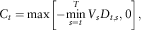 $$C_{t} =\max \left[ {{\minus}\!\mathop {\min }\limits_{s=t}^T V_{s} D_{{t,s}} ,0} \right],$$
where a floor of 0 ensures that C t is never negative.
We assume that a separate capital fund is set up with an initial capital, C 0, at time 0. At each successive valuation date t, if the sponsor is solvent:
(a) any surplus (or deficit) of the scheme, P t, is released to (or injected from) the sponsor to ensure that the scheme assets exactly equal scheme liabilities; and
(b) required capital, C t, is calculated afresh and any excess accumulated assets in the capital fund over and above C t are released back to the sponsor.
If the sponsor becomes insolvent at time t, the capital fund ensures that the eligible scheme remains self-sufficient to meet all its future obligations. Note that the formulation of C t ensures that once the initial capital fund is set up at time 0, no further capital injection is required till run-off. In other words, if the eligible scheme has sufficient assets to cover both its liabilities and required capital at time 0, the accumulated total assets will always exceed scheme liabilities till run-off.
A schematic diagram showing all the relevant cash flows of an eligible scheme is given in Figure 1.

Figure 1 The cash flow structure for an eligible scheme.
3.4. Capital requirement of PPF
To calculate PPF’s required capital, we use the same notations, as introduced in section 3.2, but adapt net cash flow, X t, to reflect PPF-specific cash flows, i.e., levies collected from eligible schemes, transferred assets of insolvent schemes, compensations paid out to transferred schemes’ members and expenses. Profits (or losses) are retained within (or paid out from) the PPF itself.
A schematic diagram of all the cash flows relevant to PPF is shown in Figure 2. As can be seen from the figure, we have persisted with the notion of a “sponsor”, even though for PPF there is none. In this context, the “sponsor” can be thought of as a hypothetical entity, providing capital to back PPF’s risks.
Figure 2 The cash flow structure for the Pension Protection Fund (PPF).
To quantify PPF’s economic capital, the relevant question is whether its accumulated assets are large enough to accommodate the maximum aggregate loss that can arise in the future. This is formalised by the following formulation of PPF’s capital requirement, C t at time t (0≤t≤T):
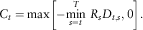 $$C_{t} =\max \left[ {{\minus}\!\mathop {\min }\limits_{s=t}^T \,R_{s} D_{{t,s}} ,0} \right].$$
At time 0, a separate capital fund is set up with an initial capital amount of C 0. At each valuation date, surplus (or deficits) are retained within PPF and excess assets are allowed to build up over time. In parallel, the capital fund is maintained in such a way that, at time t, the aggregate of the capital fund and the accumulated surplus within PPF meets the required capital amount of C t. Any excess accumulated capital is periodically released.
We have used different approaches to calculate capital requirement of eligible schemes and the PPF to capture the fundamental differences between the two funding philosophies. On one hand, solvent sponsors are fully responsible for meeting any deficits in eligible schemes; but in return any surplus can also be notionally released, e.g., through contribution holidays. However, PPF, with an aim to achieve self-sufficiency, needs to meet any deficits from funds built up from its own preceding surpluses.
3.5. Economic capital requirement
The required capital calculated in sections 3.3 and 3.4 are based on a single realisation of the future. Generalising the notions to multiple realisations provides a distribution of required capital, C t, at each time t. Economic capital requirement at time t is then defined as ρ(C t), where ρ(·) is a specific risk measure. For the purpose of this paper, we have chosen to use the value-at-risk measure. So, economic capital, ρ(C t) at confidence level p, signifies the amount of capital required at time t, to ensure that the scheme under consideration remains solvent till run-off with probability p under multiple projections of the underlying stochastic model.
Value-at-risk is a standard risk measure used by most financial services firms and is consistent with the approaches proposed in Basel 2 and Solvency 2. However, limitations of value-at-risk, as a risk measure, are well documented (see e.g. McNeil et al., 2005). Moreover, there are other risk measures, such as conditional tail expectation or tail value-at-risk, which have their own advantages and disadvantages. We are of the opinion that as long as the entire distribution of capital requirement, C t, can be estimated, one can choose to employ any risk measure and interpret the results in the light of the chosen risk measure.
Specifically, for the purposes of this paper, economic capital has been quantified as the value-at-risk at p=0.995, i.e., 99.5% confidence level, using 100,000 simulations of the underlying stochastic model.
4. Stochastic Model
There are many stochastic models available in actuarial literature, and elsewhere, which we could have used for our purposes. In this paper, we adopt the stochastic economic model of Porteous et al. (Reference Sweeting2012) and the stochastic mortality model of Sweeting (Reference Sweeting2008) to provide a full stochastic framework for economic capital calculation. These models are relatively straightforward and easy to implement, whilst still capturing the key features of the variables of interest.
4.1. Economic variables
Porteous et al. (Reference Sweeting2012) model is a subset of a much bigger model proposed by Porteous & Tapadar (2005, Reference Stevens, Waegenaere and Melenberg2008a, Reference Sweeting2008b). This model incorporates the principles of graphical structure to explain very high dimensional dependency relationships using low-dimensional clusters, or cliques, which makes it easy to implement these models. It is also capable of producing heavy-tailed distributions and tail dependence that are consistent with real-world observations. Porteous & Tapadar (2005) provides evidence that this model generates broadly similar economic capital amounts to those determined by an equivalently calibrated Wilkie (Reference Wilkie1995) model, which has been very extensively tested and used for modelling economic variables.
The main economic random variables of our stochastic model are depicted in Figure 3. The stochastic model is a standard multivariate Normal first-order autoregressive time series model, used to model yields and growth rates.
Figure 3 Graphical model of the economic variables. RPI, Retail price index.
The economic random variable, Z it, for ith variable at time t, are modelled as:
 $$Z_{{it}} =\mu _{i} {\plus}Y_{{it}} ,\;{\rm where}\;Y_{{it}} =\beta _{i} Y_{{i(t{\minus}1)}} {\plus}{\varepsilon}_{{it}} .$$
The error terms  $${\varepsilon}_{{it}} \!\sim \!N\left( {0,\sigma _{i}^{2} } \right)$$
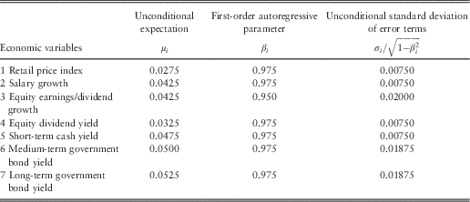
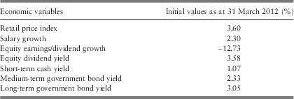
and are assumed to be independently distributed across time t. Table 1 shows the parameterisation of the individual economic random variables. Note that the stochastic economic model generates variables at monthly time intervals, which are then used to produce the annual cash flows and balance sheets for all schemes.
$${\varepsilon}_{{it}} \!\sim \!N\left( {0,\sigma _{i}^{2} } \right)$$
and are assumed to be independently distributed across time t. Table 1 shows the parameterisation of the individual economic random variables. Note that the stochastic economic model generates variables at monthly time intervals, which are then used to produce the annual cash flows and balance sheets for all schemes.
Table 1 Economic model parameterisation.
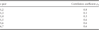
As discussed in Porteous et al. (Reference Sweeting2012), the multivariate dependency structure of the variables is handled using a graphical model approach. The error terms of the economic random variables, which are directly connected to each other in Figure 3, are dependent, with the assumed constant correlation coefficient values, ρ ij, as set out in Table 2. The error terms of economic random variables, which are indirectly connected in Figure 3, via other direct connections, are still statistically dependent, but more weakly so. For a more detailed discussion of this model, please refer to Porteous et al. (Reference Sweeting2012) and Porteous & Tapadar (2005, Reference Stevens, Waegenaere and Melenberg2008a, Reference Sweeting2008b). Graphical models are discussed in detail in Lauritzen (Reference McCarthy and Neuberger1996).
Table 2 Correlation coefficients of error terms.
The initial values of the economic variables, as at 31 March 2012, are given in Table 3. The rates for cash and government bond yields are obtained from Bank of England website (http://www.bankofengland.co.uk/statistics/Pages/yieldcurve/archive.aspx). Retail price index (RPI) figure is obtained from the “Consumer price indices” (Office for National Statistics, 2012a) and salary inflation figure is taken from “Labour market statistics” (Office for National Statistics, Reference Porteous and Tapadar2013a). Initial values for equity dividend yield and earnings growth are derived from FTSE All Share Indices obtained from http://markets.ft.com.
Table 3 Initial values of economic variables as at 31 March 2012.
4.2. Demographic variables
The longevity risk inherent in DB pension schemes stems from the uncertainty surrounding estimates of mortality improvements over potentially many decades into the future. This has huge implications for DB pension scheme costs, value of liabilities and economic capital requirements.
Cairns et al. (Reference Cairns, Blake, Dowd, Coughlan, Epstein, Ong and Balevich2009), and references therein, provides a rich literature on stochastic mortality models and any of these models could have been used in our modelling work. However, we follow the approach used in Porteous et al. (Reference Sweeting2012) to use Sweeting (Reference Sweeting2008) in conjunction with standard mortality tables published by the Institute and Faculty of Actuaries, as this would be consistent with most actuarial valuations carried out by eligible schemes.
The mortality model used in this paper is developed in three steps:
Step 1: we choose S1PM and S1PF as the baseline mortality tables for males and females, respectively, as published by the Institute and Faculty of Actuaries in their Continuous Mortality Improvement (CMI) Working Paper No. 34 (Institute and Faculty of Actuaries, 2008).
Step 2: we then project these base mortality tables from year 2006 to year 2012 using the mortality projection table published by the Institute and Faculty of Actuaries in their CMI Working Paper No. 63 (Institute and Faculty of Actuaries, 2013).
Step 3: finally, we model the future stochastic mortality improvements starting from 2012 using the approach of Sweeting (Reference Sweeting2008), who has developed a pragmatic method of modelling stochastic uncertainty around a central mortality projection. Specifically, if q x,f denotes the central projection of mortality rate for future year f and age x, the logit of central mortality rate is defined as:
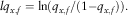 $$lq_{{x,f}} =\ln (q_{{x,f}} /(1{\minus}q_{{x,f}} )).$$
Then the logit of the stochastic mortality rate, modelling future uncertainty, is defined as:
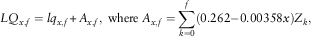 $$LQ_{{x,f}} =lq_{{x,f}} {\plus}A_{{x,f}} ,\;{\rm where}\;A_{{x,f}} =\mathop{\sum}\limits_{k=0}^f (0.262{\minus}0.00358x)Z_{k} ,$$
and Z k is independent standard normal variable.
Sweeting’s (Reference Sweeting2008) proposed stochastic mortality fluctuations are based on England and Wales male lives aged 50–90. We have used the same approach for all members in our model.
5. Model Assumptions
To quantify economic capital for eligible schemes and PPF, in addition to the stochastic models for economic and demographic projections discussed in section 4, we need to develop a high-level model of the UK DB pension sector to project the assets and liabilities of the eligible schemes and also the PPF. The modelling assumptions relevant for all schemes are provided in this section. Some additional assumptions that are specific to the PPF are discussed in section 7.
5.1. Benefit structure
We assume that all schemes take the same generic final salary DB pension benefit structure where the normal retirement age is assumed to be 65 for both males and females. Early and late retirements are not considered as these options are roughly cost-neutral.
5.1.1. Eligible schemes pension benefits
Pensions and cash lump sum benefits on retirement is calculated using an accrual rate of 80ths (giving a pension of half the final salary after 40 years of service) plus a lump sum of three times the annual pension, i.e.:
 $${\rm Annual}\,{\rm pension}={\rm Accrual}\,{\rm rate}{\times}{\rm Pensionable}\,{\rm service}{\times}{\rm Pensionable}\,{\rm salary,}$$
 $${\rm Lump}\,{\rm sum}\,{\rm payment}={\rm 3}{\times}{\rm Annual}\,{\rm pension,}$$
where pensionable service denotes the duration of employment and pensionable salary is the final salary at the date of retirement. The annual pension is assumed to increase in line with RPI as generated by the stochastic economic model discussed in section 4.1.
The particular choice of accrual rate is based on the findings of “Chapter 6 of pensions trends” (Office for National Statistics, Reference Porteous, Tapadar and Yang2013b). According to this report, in 2011, a majority of the DB scheme members (84% of public sector and 64% of private sector scheme members) were accruing benefits at an accrual rate of 80ths plus an additional lump sum at retirement of three times the annual pension or at 60ths without a lump sum payment. Both structures are deemed to be broadly comparable in terms of benefits. To avoid too many variables in the model, we have chosen to only model the accrual rate of 80ths plus lump sum at retirement to represent all schemes. However, we acknowledge that an accrual rate of 60ths would have produced a higher economic capital.
The age and gender-specific salary distributions of eligible scheme members, as at 31 March 2012, are assumed to follow the promotional salary scale of LG59/60 table with an average annual earnings of £26,500, which is consistent with the average earnings in the United Kingdom, as reported in the “Annual survey of hours and earnings, 2012 provisional results” (Office for National Statistics, Reference Olivieri and Pitacco2012b). LG59/60 promotional salary scale is widely used for actuarial valuation of eligible schemes (see e.g. the 2011 actuarial valuation of the superannuation arrangements of University of London; SAUL, 2012).
Future salary increases are assumed to follow the salary inflation generated by the stochastic economic model discussed in section 4.1.
5.1.2. Eligible schemes death benefits
Scheme death benefits are assumed to be as follows:
∙ For active members, death in service benefits comprise a lump sum payment of three times annual salary and a spouse’s pension of half the pension that the member would have received if the member had survived until normal retirement.
∙ On the death of a deferred pensioner, a lump sum equal to the present value of the deferred lump sum payable at normal retirement age is provided along with a spouse’s pension of half the amount of the deferred pension at date of death.
∙ On the death of a pensioner, a spouse’s pension equal to half the member’s pension is paid to the surviving spouse.
This is broadly in line with the benefit structure of the USS, which is one of largest DB schemes in the United Kingdom.
The proportions of married scheme members for relevant ages and gender are assumed to follow the trends of the general UK population as published in the “Population estimates by marital status, mid 2010” (Office for National Statistics, 2011). For simplicity, we have assumed that for a married couple, husband and wife are of the same age.
5.1.3. Eligible schemes withdrawal benefits
For members withdrawing from an eligible scheme, deferred RPI-linked pension benefits are provided based on accrued service on withdrawal. RPI indexation of salaries between the date of leaving and retirement is provided.
Although withdrawal experience would normally vary between schemes, for simplicity we have assumed the same withdrawal rates for all eligible schemes, set at 270% and 113% of the LG59/60 withdrawal rates for males and females, respectively. This is the assumption used for the 2011 actuarial valuation of the USS (2012).
5.1.4. PPF schemes compensations
Our assumptions on PPF compensations are based on PPF’s 2011/2012 “Annual report and accounts” (The Pension Protection Fund and The Pensions Regulator, 2012a). According to this document, PPF operates two levels of compensation for members of schemes that are transferred to the PPF.
For members who have already retired or are in receipt of survivor pensions before the transfer date, PPF pays 100% of pensions in payment.
For other members, including active and deferred members on the transfer date, PPF pays 90% of pensions in deferment, subject to an age-adjusted compensation cap, which, on 31 March 2012, was £34,049.84/annum at age 65. This deferred compensation is revalued annually in line with inflation between the date of transfer and the date of compensation commencement, where the annual increase is subject to a cap of 5% for compensation linked to pensionable service before 6 April 2009, and a cap of 2.5% in respect of compensation linked to pensionable service on or after 6 April 2009.
For pensions in payment, PPF increases the part of the compensation relating to pensionable service from 5 April 1997 in line with inflation, subject to a maximum of 2.5%/annum. Compensation relating to service before that date is not increased.
For future projections of PPF benefits, we will use the RPI variable generated by the stochastic economic model as discussed in section 4.1. Although PPF has moved from retail price to consumer price indexation of benefits from 2011, we will not make this distinction in this paper.
5.2. Valuation of liabilities
As discussed in section 3.1, we will use s179 liability valuation approach for the purposes of this paper. The discount rates for calculating s179 liabilities are prescribed in regulations and are complex functions of yields on a number of UK fixed interest and index-linked bond indices. Details on the different discount rates used for the 2012 actuarial valuation of the PPF are given in PPF’s 2011/2012 “Annual report and accounts” (The Pension Protection Fund and The Pensions Regulator, 2012a).
In our paper, to calculate s179 liabilities, we propose a simplified approach of using a discount rate linked to the long-term government bond yield generated by the stochastic economic model described in section 4.1. First, we note that the long-term government bond yield on 31 March 2012 was 3.05% as set out in the initial values in Table 3. Then, based on all the different discount rates used in the 2012 actuarial valuation of the PPF (The Pension Protection Fund and The Pensions Regulator, 2012a), we obtain an average rate of 2%, i.e., 65% of the long-term government bond yield, which provides a very good fit for the model points developed in section 5.3.1. For calculating s179 liabilities at future valuation dates, we use a discount rate of 65% of the long-term government bond yield generated by the stochastic model discussed in section 4.1.
5.3. Model points
5.3.1. Eligible schemes
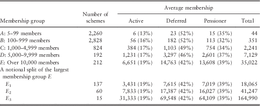
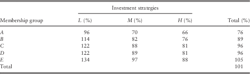
To represent membership profiles of eligible schemes, we propose a realistic but simple high-level model based on publicly available data. According to The Purple Book 2012 (The Pension Protection Fund and The Pensions Regulator, 2012b), as at 31 March 2012, there were 6,316 eligible schemes with a total of 11.7 million members. The number of schemes and the average profile of each membership group are given in Table 4.
Table 4 Average membership profile of eligible schemes.
Although there were only 212 schemes in group E, it has more members than that of all the other groups put together. So, the impact of an insolvency event of one of these large schemes can have far-reaching consequences for the PPF. In order to capture this feature, we have notionally sub-divided the membership group E into three sub-groups E 1, E 2 and E 3, also shown in Table 4. The total membership of group E is equally split between the three sub-groups, but the number of schemes in each sub-group is allocated notionally, broadly based on the data from the Top 100 Pension Schemes 2010 (Professional Pensions, 2010) document. As can be seen from Table 4, the variation of membership profiles within the sub-groups of membership group E can be large and can have a significant bearing on the overall risk assessment of the PPF.
To keep the modelling simple, we assume that every eligible scheme within the same membership group is identical, with the same average profile as given in Table 4.
For all membership groups, male and female active members are assumed to be uniformly distributed across ages between 25 and 65, represented by ages 30, 40, 50 and 60. Deferred members and pensioners are represented by single ages 50 and 70, respectively, for both genders. The gender composition is assumed to be 66% males and 34% females for all categories. The age assumption for deferred members and pensioners, as well as the gender composition of eligible schemes, are consistent with the data on PPF schemes available in PPF’s 2011/2012 “Annual report and accounts” (The Pension Protection Fund and The Pensions Regulator, 2012a).
Past service for active members, accrued pension for deferred members and annual pension for pensioners are modelled by calculating the s179 liabilities using a discount rate of 2%/annum, as discussed in section 5.2. The fitted model points are given in Table 5. Table 6 shows that the fit of the model points to the PPF data is very good.
Table 5 Eligible schemes model points.
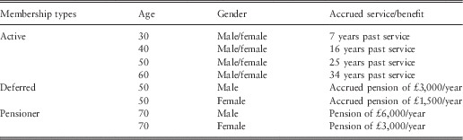
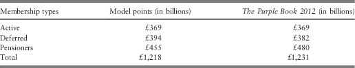
Table 6 Comparison of s179 liabilities between model points and The Purple Book 2012.
We will not consider new entrants to the eligible schemes. Instead, we will focus entirely on the risk profile of the existing members of the UK DB pension sector including schemes under PPF assessment, as at 31 March 2012.
5.3.2. PPF schemes
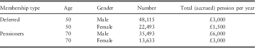
For schemes transferred to the PPF, the members, by definition, are either deferred or pensioners. From the PPF’s 2011/2012 “Annual report and accounts” (The Pension Protection Fund and The Pensions Regulator, 2012a), the actual average ages for PPF schemes deferred members are 49.5 and 47.8 for males and females, respectively, while those for pensioners are 68.4 and 67.8 for males and females, respectively. To maintain consistency with the eligible schemes’ model points, for PPF schemes we use the same model points of age 50 for deferred members and age 70 for pensioners for both genders. Table 7 shows the PPF schemes model points along with the number of members and accrued benefits as at 31 March 2012.
Table 7 Pension Protection Fund schemes model points.
5.4. Funding levels and asset allocation
5.4.1. Eligible schemes
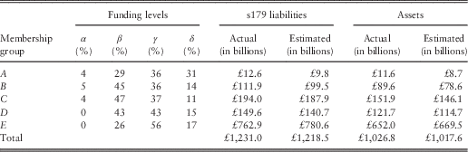
For projecting eligible schemes’ assets forward in the future, we need the starting level of scheme assets, as at 31 March 2012. Although this information is not directly available, The Purple Book 2012 (The Pension Protection Fund and The Pensions Regulator, 2012b) provides total s179 liabilities for each membership group A–E, and the distribution of funding levels (as percentages of s179 liabilities). The schemes are classified according to 0–50%, 50–75%, 75–100% and over 100% funding levels, which we assume to be represented by average funding levels of 45%, 65%, 85% and 120%, respectively, and denoted by α, β, γ and δ, respectively, for ease of reference.
The distribution of eligible schemes according to funding levels, in each membership group, is given in Table 8. Table 8 also provides the estimated total assets and s179 liabilities for each membership group based on this assumption, which shows a very good fit to the actual levels of assets, again taken from The Purple Book 2012 (The Pension Protection Fund and The Pensions Regulator, 2012b).
Table 8 Actual and estimated s179 liabilities and total assets of eligible schemes by membership groups and funding levels.
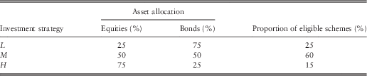
According to The Purple Book 2012 (The Pension Protection Fund and The Pensions Regulator, 2012b), in each year between 2006 and 2012, >80% of all eligible schemes’ assets are invested in a combination of equities and bonds. So, in this paper, we will focus entirely on equities and bonds. However, actual allocation of assets between equities and bonds vary from scheme to scheme. We propose a simple model with three possible investment strategies: L (low equity/high bond investment strategy), M (equal equity and bond investment) and H (high equity/low bond investment strategy), broadly based on the asset allocation distribution given in The Purple Book 2010 and The Purple Book 2011, as this particular piece of information was not included in The Purple Book 2012 (The Pension Protection Fund and The Pensions Regulator, 2012b). Table 9 shows the modelled asset allocation strategies along with the proportion of eligible schemes adopting these strategies.
Table 9 Distribution of eligible scheme by investment strategies.
5.4.2. PPF schemes
To project PPF’s assets forward in the future, the starting level of assets, as at 31 March 2012, is £11.139 billion according to PPF’s 2011/2012 “Annual report and accounts” (The Pension Protection Fund and The Pensions Regulator, 2012a). The corresponding s179 liability was £8.375 billion giving a surplus of £2.764 billion.
According the PPF’s “Statement of investment principles” (The Pension Protection Fund and The Pensions Regulator, 2012c), PPF aims for a strategic asset allocation of 70% in fixed interest (cash and bonds), 10% in equities and 20% in alternatives, including properties. As our focus in this paper is only on equity and bond investments, we will assume that PPF’s assets are invested in 25% equities and 75% bonds, making it consistent with eligible schemes’ investment strategy L, defined in section 5.4.1
5.5. Eligible schemes’ contribution rates
Using projected unit method on the active membership profile for all eligible schemes, we obtain an average standard contribution rate of 23.2% of an active member’s annual salary. Although the contribution rate will usually vary from scheme to scheme and from year to year based on the membership profile and investment strategy, we use the same average contribution rate for all schemes for modelling simplicity.
5.6. Expenses
For all schemes, we use the same expense assumption of:
(a) a fixed annual expense of £60 per member, increasing in line with RPI as generated by the stochastic economic model; and
(b) a variable expense of 0.1% of the fund under management per annum.
This assumption is based on Porteous et al. (Reference Sweeting2012), who use these expense assumptions to calculate economic capital for USS.
6. Eligible Schemes Results
In this section, we quantify economic capital of eligible schemes, based on the technique outlined in section 3.3. For presentation purposes, we will extend the notations developed in section 3 as follows:
-
$L_{t}^{X} $
denotes the s179 liability at time t of an eligible scheme in membership group X;
-
$\rho _{t}^{{XY}} $
denotes the economic capital requirement at 99.5% confidence level at time t of an eligible scheme in membership group X pursuing investment strategy Y;


where X=A, B, C, D, E 1, E 2, E 3 and Y=L, M, H. Note that s179 liability of an eligible scheme is not affected by the scheme’s investment strategy.
6.1. Eligible schemes’ economic capital requirement as at 31 March 2012
Table 10 shows economic capital requirements, as percentages of s179 liabilities, as at 31 March 2012, for all membership groups and for different investment strategies, i.e.,  $$\rho _{0}^{{XY}} /L_{0}^{X} $$
, where 31 March 2012 is referred to as time t=0. As the split between active/deferred/pensioner memberships is assumed to be the same for E 1, E 2 and E 3, the economic capital requirements, as percentages of s179 liabilities, are the same for all these three sub-groups and are shown against the consolidated group E in the table.
$$\rho _{0}^{{XY}} /L_{0}^{X} $$
, where 31 March 2012 is referred to as time t=0. As the split between active/deferred/pensioner memberships is assumed to be the same for E 1, E 2 and E 3, the economic capital requirements, as percentages of s179 liabilities, are the same for all these three sub-groups and are shown against the consolidated group E in the table.
Table 10 Eligible schemes’ economic capital as percentages of s179 liabilities, for all membership groups and for different investment strategies, as at 31 March 2012.
We observe the following:
(a) The aggregate economic capital requirement of all eligible schemes is 101% of the aggregate s179 liabilities. In other words, if UK eligible schemes were required to hold economic capital, as is the case for the UK insurers, an additional aggregate amount of £1,231 billion capital will be needed on top of the aggregate s179 liabilities. Note that as at 31 March 2012, the eligible schemes had assets worth £1,026.8 billion, which does not even cover the s179 liabilities.
(b) Economic capital requirements, as at 31 March 2012, range from 66% to 134% of s179 liabilities depending on scheme sizes and investment strategies pursued. This is broadly in line with the findings of Porteous et al. (Reference Sweeting2012), who report an economic capital requirement of 60% of best-estimate liabilities for USS. Note that, USS falls in membership group E with a very high 90% equity investment strategy.
(c) Economic capital requirements, as at 31 March 2012, as percentages of s179 liabilities, broadly increase with the size of the membership group. This trend is explained by the increasing proportion of active members in the larger schemes, as can be seen in Table 4. Higher proportions of active members means larger benefit payments far into the future, leading to greater risk, thus requiring higher economic capital backing.
(d) Economic capital requirements, as at 31 March 2012, as percentages of s179 liabilities, increases with greater bond investments, for the strategies L, M and H. This is consistent with the findings of Porteous et al. (Reference Sweeting2012), who reported similar findings. The pattern can be explained by analysing the evolution of economic capital requirements over the entire run-off of eligible schemes as discussed in section 6.2.
6.2 Eligible schemes’ economic capital requirement over entire run-off
Figure 4 shows the s179 liabilities and economic capital requirements for different investment strategies for two representative schemes – one from the smallest membership group A and the other from the largest group E 3.
Figure 4 Liability and economic capital requirements for different investment strategies of an eligible scheme in each of the membership groups A and E 3.
We make the following observations:
(a) As the mortality model assumptions, outlined in section 4.2, provides mortality rates for up to 120-year olds, the projection period stretches until 2102, when the last of the current 30-year-old active members die.
(b) The shapes of the s179 liabilities and economic capital graphs are broadly similar for both schemes but the magnitudes are vastly different. For the scheme in group A, s179 liabilities start at around £4 million, while for the group E 3 scheme, it starts at >£17 billion. Similarly, the economic capital graphs, for the group A scheme, reach a maximum of approximately £10 million at around year 2040, while for the scheme in group E 3, the maximum is >£50 billion.
(c) The s179 liabilities curves increase in the initial years, as the active members continue accruing benefits, but fall subsequently as the members eventually age and die. The kinks in the s179 liability curves are owing to the model points assumptions that, on 31 March 2012, active members are all aged either 30, 40, 50 or 60, while deferred members are all aged 50. As cash lump sums are paid out on members’ retirements in the years 2017, 2027, etc., the liabilities fall sharply in those years, producing the kinks. The largest fall is in the year 2027 when the current 50-year-old active and 50-year-old deferred members retire all together.
(d) The shapes of the economic capital graphs are characteristics of the method outlined in section 3.3. The economic capital requirements are negligible near the end of the run-off period, as the future risk inherent in the benefit payments of the few remaining surviving members is insignificant. Working backwards through time, the economic capital requirements are highest at around year 2040. The lower economic capital requirements, in the years before 2040, can be interpreted as funds to be set aside to attain the maximum economic capital requirement at around year 2040.
(e) Investment strategy H, with the highest equity content, produces the highest peaks of economic capital requirement among the investment strategies L, M and H, as expected. However, higher expected returns for investment strategy H compensates for this by requiring relatively smaller economic capital initially. On the other hand, investment strategy L, with the highest bond content, produces a lower peak but a larger economic capital requirement in the initial years. Investment strategy M, with equal bond and equity investment, produces the smallest peak along with an initial economic capital requirement, which is only slightly higher than that of H and significantly lower than that of L. So, it can be seen that the choice of investment strategy can have a significant bearing on an eligible scheme’s risk profile and economic capital requirement.
In Figure 4, we have not shown the s179 liabilities and economic capital requirements for all membership groups, as all these graphs are qualitatively similar. Instead, in Figure 5, we present the scaled s179 liabilities and economic capital requirements graphs, in order to make consistent comparisons.
Figure 5 Liabilities and economic capital of eligible schemes as proportions of the liability values as at 31 March 2012, shown as multiple of the corresponding values for the membership group A.
First, we divide the s179 liabilities,  $L_{t}^{X} $
, and economic capital requirements,
$L_{t}^{X} $
, and economic capital requirements,  $$\rho _{t}^{{XY}} $$
, by the relevant s179 liabilities at time 0,
$$\rho _{t}^{{XY}} $$
, by the relevant s179 liabilities at time 0,  $L_{0}^{X} $
, for each membership group X and investment strategy Y. Then in Figure 5, we present the resulting scaled values as a multiple of that of a scheme from group A. As the scaled s179 liabilities and economic capital requirements are the same for all three sub-groups E 1, E 2 and E 3, we present these results for the consolidated group E.
$L_{0}^{X} $
, for each membership group X and investment strategy Y. Then in Figure 5, we present the resulting scaled values as a multiple of that of a scheme from group A. As the scaled s179 liabilities and economic capital requirements are the same for all three sub-groups E 1, E 2 and E 3, we present these results for the consolidated group E.
We make the following observations:
(a) Group E scheme’s scaled s179 liabilities are the highest in the long run, as these schemes have the highest proportion of active members. Schemes in groups C and D have broadly the same proportion of active members, but group C has a higher proportion of deferred members, which explains a slightly higher scaled s179 liabilities compared with that of a group D scheme. Group A schemes have the least proportion of active numbers, followed by group B, which is evident from the relative positions of the scaled liability curves for these two groups.
(b) The scaled economic capital requirement graphs are also affected by the proportion of active members in a membership group. Group E has the highest number of active members implying highest risk and the highest scaled economic capital requirement. Groups C and D are broadly similar in their scaled economic capital requirement. Group B has lower proportion of active members compared with the schemes in groups C, D and E resulting in a lower scaled economic capital requirement. Group A has the lowest risk profile.
(c) Both the scaled s179 liabilities and economic capital requirements beyond 2082 become fixed as multiples of the respective values for a group A scheme, because all pensioners currently aged 70 and deferred members currently aged 50 dies by then. Beyond 2082, the relative differences in the schemes are only because of the proportion of current active members aged 30 and 40 in the respective schemes.
7. PPF Results
In this section, we quantify PPF’s economic capital using the technique outlined in section 3.4. For this purpose, we need to discuss some further assumptions, which are specific to PPF, in addition to the ones already mentioned in section 5.
7.1. PPF-specific assumptions
7.1.1. PPF levy
PPF collects annual levies from all eligible schemes to cover the insolvency risks of the sponsors. The levy is made up of two parts – a scheme-based part based on a scheme’s total s179 liabilities and a risk-based part based on under-funding risk and probability of sponsor insolvency. The exact formulation of the levy has been a subject of substantial debate and has been updated a number of times. For the purposes of this paper, we make a simplified assumption that the aggregate levy collected is a constant proportion, c, of the total s179 liabilities of all eligible schemes. We have also checked (not shown here) that PPF’s economic capital is not sensitive to the levy assumption.
We estimate the parameter c using the principle that the aggregate levy charged should be just enough for PPF to meet the total expected deficit arising from transferred schemes with insolvent sponsors. We have used our stochastic model, discussed in section 4, to simulate future deficits transferred to the PPF and future total s179 liabilities of eligible schemes. An estimate of c=0.072% is obtained by equating the expected net present value of levies to future deficits.
The above estimate of c is broadly consistent with the data available from The Purple Books, which shows the actual average levies charged were 0.069%, 0.066%, 0.067%, 0.068% and 0.048% of the total s179 liabilities for the years 2008–2012.
7.1.2. Insolvency rates of sponsors of eligible schemes
For calculating economic capital of eligible schemes, we ignored sponsor insolvencies. As an eligible scheme is solely dependent on the existence and solvency of a single entity, i.e., its own sponsor, the laws of probability do not apply. So our economic capital calculation approach for eligible schemes is designed to ensure that the scheme stays solvent, irrespective of the future solvency status of its sponsor. Note that we do not consider multi-employer schemes in this paper.
However, existence of more than 6,000 eligible schemes makes the assumption on sponsor insolvency rates crucial for quantifying PPF’s economic capital.
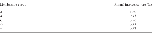
For our model, the average annual insolvency rates of sponsoring employers of eligible schemes are taken from The Purple Book 2012 (The Pension Protection Fund and The Pensions Regulator, 2012b) and reproduced in Table 11. For future projections, we have assumed that the number of annual defaults for each membership group follow Poisson distribution with parameters set at the average rates. We also assume that sponsor insolvency events are independent of each other and also across years.
Table 11 Average annual insolvency rates of sponsors of eligible schemes.
7.1.3. Eligible schemes’ amortisation period and funding cap
Reflecting current practice, our starting base assumption is that eligible schemes themselves are not specifically required to set aside economic capital. However, during the projection period, if the value of a scheme’s assets fall below the level of s179 liabilities, the scheme is required to make up the deficit over an amortisation period of 10 years.
We also impose a maximum funding cap of 120% of s179 liabilities, to prevent eligible schemes from building up excessive surpluses and using them as tax avoidance devices. This assumption is consistent with McCarthy & Neuberger (Reference McCarthy and Neuberger2005a). If, during the projection period, eligible schemes’ assets exceed the funding cap, the surplus is assumed to be released back to the sponsor.
7.2. Base case results
Based on these assumptions, Figure 6 shows the evolution of PPF’s liability and economic capital from 2012 till run-off. Henceforth, this will be referred to as the base case result. PPF’s liability starts at around £8 billion in 2012 (consistent with the number reported in the PPF’s 2011/2012 “Annual report and accounts”; The Pension Protection Fund and The Pensions Regulator, 2012a), before reaching its peak of about £150 billion in 2050 and finally falling to 0.
The base case economic capital in 2012, is approximately £35 billion, rising to around £75 billion in 2030. Economic capital falls to 0 soon after 2050, implying that by then PPF would have accumulated enough additional assets within its own fund to sustain itself going forward and thus explicit backing of economic capital is not required any further.
In reality, PPF’s 2011/2012 “Annual report and accounts” (The Pension Protection Fund and The Pensions Regulator, 2012a) shows a surplus of <£3 billion, which when compared against an economic capital of £35 billion, reflects a substantial deficit in economic capital required to back the true underlying risks involved.
However, to keep matters in perspective, recall from the results in section 6, that if each individual eligible scheme is required to hold economic capital, then the entire sector would be required to raise >£1,200 billion of additional capital in aggregate. As an alternative, a shortfall of £32 billion in PPF’s economic capital appears reasonable. This huge reduction in the order of magnitude in economic capital amount is primarily because of the incorporation of sponsor insolvency rates in PPF’s economic capital calculation. In other words, large diversification benefits can be achieved by pooling of risks across different sponsor profiles and membership groups.
As can be appreciated, we have made a large number of assumptions to calculate PPF’s base case economic capital. So, it is important to analyse the sensitivity of the base case result to a number of key variables. These are presented in the rest of this section. Figure 6 also shows PPF’s economic capital in 2012 for the base case (shown by the vertical dotted line at £35 billion) and other scenarios for which sensitivity analysis have been carried out.
7.3. Impact of eligible scheme funding levels and amortisation period
The base case PPF result does not require eligible schemes to hold any more than the s179 liabilities with a funding cap of 120% of s179 liabilities. In addition, a 10-year amortisation period is applied for schemes in deficit. So in this section, we check the following scenarios:
(a) We increase the cap of 120% maximum funding level to 150%. As shown in Figure 6, PPF’s economic capital, in this scenario, falls from £35 to £23 billion in 2012. In Figure 7, the evolution of PPF’s liabilities and economic capital shows that the liability curve has a substantially lower peak at approximately £60 billion. The economic capital also peaks at a lower value of around £50 billion, and falls to 0 faster. The increased funding cap ensures that more eligible schemes would be in surplus if and when their sponsors become insolvent, requiring fewer schemes being transferred to PPF.
(b) A more pro-active alternative to increasing the funding cap is to require eligible schemes to build up a specified amount of buffer assets over the amortisation period. For buffers of 50% and 100% of s179 liabilities, Figure 6 shows substantial relief in PPF’s economic capital requirements in 2012, which fall to £21 and £14 billion, respectively. The evolution of economic capital, in Figure 7, shows that requiring a 50% buffer has a bigger impact than increasing the maximum funding cap to 150%. Incidentally, a 100% buffer is broadly equivalent to requiring eligible schemes to hold economic capital, as quantified in section 6. Figure 7 shows that a requirement of 100% buffer means a significant reduction in PPF’s economic capital, which never exceeds £25 billion and falls to 0 much faster. However, note that even a 100% buffer will not completely eliminate PPF’s economic capital requirement as:
(1) PPF would still require economic capital for schemes already transferred to PPF;
(2) PPF still bears the risk of scheme insolvencies during the amortisation period over which the buffer requirement is met;
(3) different eligible schemes have different risk profiles and thus different economic capital requirement, which is not consistent with a blanket requirement of 100% buffer, for all eligible schemes.
(c) Finally, in this section, we look at the impact of amortisation period, by reducing it from 10 to 4 years. PPF’s economic capital requirement drops to £25 billion (Figure 6) in 2012 and it also fallsto 0 sooner (Figure 7).
However, a dramatic impact is observed in Figures 6 and 7, when the amortisation period of 4 years is imposed in conjunction with a buffer requirement. In this case, PPF’s economic capital in 2012 falls below £15 and £10 billion for buffer requirements of 25% and 50%, respectively. In addition, PPF’s requirement of economic capital backing would cease much earlier than 2040.
Figure 6 Pension Protection Fund’s (PPF) base case liability and economic capital requirements and PPF’s economic capital requirements as at 31 March 2012 for different scenarios.
This analysis shows that a judicious mixture of a shorter amortisation period and a reasonable buffer requirement for eligible schemes can bring down PPF’s underlying risk and economic capital requirement drastically.
7.4. Impact of asset allocation strategy
The base case PPF result assumes the investment strategy that 75% of PPF’s assets are invested in bonds while 25% are in equities, which is equivalent to investment strategy L defined in section 5. In this section, we analyse the impact of asset allocation strategy on PPF’s economic capital requirement by looking at alternative investment strategies, M (50/50 in bond/equity) and H (25/75 in bond/equity).
To maintain consistency, PPF levies needs to be recalculated to reflect the long-term returns of the alternative investment strategies. The revised PPF levies are 0.066% and 0.061% for strategies M and H, respectively. Recall from section 7.1.1 that PPF levy for base case investment strategy L was set at 0.072%.
Figure 6 shows that the impact on economic capital requirements are relatively modest in 2012, at £32 and £39 billion for strategies M and H, respectively. Figure 8 shows that PPF’s liabilities are unaffected by the choice of investment strategies.
Figure 7 Sensitivity of Pension Protection Fund’s liability and economic capital to maximum funding ratio, buffer requirements and amortisation period.
However, the evolution of PPF’s economic capital, shown in Figure 8 for these scenarios, shows interesting patterns. As expected, investment strategy H, with higher equity content, has a higher initial economic capital and also a higher peak compared with strategies L and M. But, economic capital for both M and H fall to 0 much earlier than that for strategy L. Between strategies L, M and H, investment strategy M seems to provide a good balance between PPF’s risk (as can be seen from its lowest overall peak) and returns (as evidenced from the shorter period of economic capital requirement).
7.5. Impact of longevity stress
In Figures 6 and 8, we also show the impact of increasing the size of the volatility (standard deviation) parameter in our stochastic mortality model, by two and five times. As expected economic capital increases everywhere. This is especially concerning given the lack of success that actuaries and others have had historically in estimating future improvements in longevity. Liabilities also increase quite significantly in the longer term. This is a feature of the stochastic mortality model we have used, where increasing the volatility causes the distribution of mortality rates to become more negatively skewed.
7.6. Impact of sponsor insolvency rates
In this section, we provide sensitivity analysis on the crucial assumption of sponsor insolvency rates. We check this by changing the base rates by +50% and −50%. The results are presented in Figures 6 and 9. A substantial impact is observed in both liabilities and economic capital over the entire duration of the projection period. In particular, a 50% increase in sponsor insolvency rates raises PPF’s economic capital requirement in 2012 by £10 billion; while a 50% reduction results in a fall of £15 billion.
Figure 8 Sensitivity of Pension Protection Fund’s liability and economic capital to investment strategy and future mortality rates.
We also observe that the insolvency rates, given in Table 11, show a strange pattern, where the membership group E has a higher sponsor insolvency rate than that of group D, which is unusual as one would expect bigger groups to have financially stronger sponsors with lower insolvency rates. So we check a scenario where E 1, E 2 and E 3, the sub-groups of the largest membership group E, have different sponsor insolvency rates. We notionally allocate insolvency rates of the sub-groups as follows. Sponsors of E 3 schemes with largest membership profile are assumed to have the lowest insolvency rates. Schemes in sub-group E 2 are assumed to have twice the insolvency rate of E 3, and the rate for E 1 being double that of E 2. Keeping the weighted average rate for the whole group E to be 0.72%, the insolvency rates for each sub-group is given in Table 12. Note that the new insolvency rate for E 1 is the same as that of group C, while E 2 and E 3 now have lower insolvency rates compared with group D.
Table 12 Average annual insolvency rate assumptions for membership sub-groups E 1, E 2 and E 3.
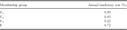
Figure 6 shows a £4 billion drop in PPF’s economic capital in 2012 and Figure 9 shows a substantial reduction throughout the projection period. This again highlights the importance of the sponsor insolvency rates assumptions for PPF’s economic capital calculation.
In this paper, we have used a simple Poisson distribution, with fixed average parameters, to model sponsor insolvencies. Given the sensitivity of the results to sponsor insolvency rates, a more comprehensive model, taking into account the dependency of these rates on relevant economic variables, would appear desirable. This will also be consistent with the experience that insolvency rates tend to increase in poor economic conditions. Incorporating such features in the model could potentially increase economic capital requirement substantially. However, we defer such a modelling approach to a future paper.
7.7. Impact of PPF taking over all schemes with insolvent sponsors
We conclude this section by focusing on one of the main underlying assumptions behind PPF’s defining role. As discussed in section 2.2, PPF only takes over schemes with insolvent sponsors, but only if they are in deficit. Schemes that are in surplus, on the date of sponsor insolvency, are not transferred to PPF. This is based on the assumption that these schemes in surplus can either continue operating on their own or secure benefits for their members with another provider using their own funds.
If a surplus scheme, with insolvent sponsor, decides to continue operating on their own, we have seen in section 6 that the surplus needs to be substantially high to meet the economic capital requirement. Alternatively, costs of securing benefits from a third party can be significantly higher than the asset values. So, in this section we investigate scenarios in which PPF takes over all schemes, with insolvent sponsors, irrespective of their funding status.
Figure 9 shows the results. It can be seen from the changes in the scales of the vertical axes that both PPF’s liability and economic capital increase substantially if PPF accepts all schemes with insolvent sponsors. In particular, all else being the same as the base case, PPF’s liability can exceed £500 billion during the run-off period, while economic capital can be as much as four times higher than the base case results.
Figure 9 Sensitivity of Pension Protection Fund’s (PPF) liability and economic capital to sponsor insolvency rates and if PPF takes over all schemes with insolvent sponsors.
Arguably, in this scenario, where PPF takes over all schemes with insolvent sponsors, the economic capital of approximately £130 billion in 2012, reflects the true underlying risk of the entire UK DB pension sector, taking PPF into account. Note that even the amount of £130 billion appears reasonable when compared with £1,200 billion, which would be required if each eligible scheme were required to hold economic capital separately.
Taking this analysis further, and based on the results of previous sensitivity analyses, we re-analysed this scenario with a shorter 4-year amortisation period in conjunction with a 50% buffer requirement. Figure 9 shows that in this case economic capital reduces substantially as expected, with a requirement of only £70 billion in 2012. Note that the liabilities are unaffected by changes in amortisation period and buffer requirements, as all schemes with insolvent sponsors are transferred to PPF. This again shows that some risk sharing across the sector, between individual eligible schemes and the PPF, can substantially reduce the risk of the entire sector.
8. Conclusions
Given the backdrop of intense scrutiny on financial risk management of firms, along with the implementation of banking and insurance regulations, in this paper, we quantify risks underlying the UK DB pension sector from an economic capital perspective. Apart from the increased regulatory interest, this is also relevant from a social policy perspective, as the UK DB pension sector shows signs of steady decline. So a proper risk assessment of the entire sector becomes paramount, so that the relevant stakeholders can make informed decisions. In particular, the impact of PPF needs to be addressed in a quantitative manner, for a holistic perspective of the entire UK DB pension sector risk.
In this paper, we have used an economic capital approach to quantify risks underlying individual eligible schemes on a stand-alone basis and also the PPF. We propose a run-off approach to quantify economic capital to capture the long-term nature of pension scheme risks. Stochastic models were used for economic and demographic variables. A high-level model of the entire UK DB pension sector was developed using publicly available information. The proposed model involves a large number of assumptions and results are based on projections over a long time horizon. So a lot of care needs to be taken to interpret the results. We suggest that more emphasis is given to the relative magnitudes, rather than absolute values, of the results.
We find that, on a stand-alone basis, economic capital for individual schemes are on average at the same level as the s179 liabilities. This translates to an aggregate requirement of £1,200 billion of additional capital for the entire sector. Although the economic capital for individual schemes can range between 66% and 134% of s179 liabilities, for most schemes it would be far too onerous. So imposition of any regulatory stand-alone economic capital requirement would need to be managed pragmatically and over an extended period. Otherwise, it will most certainly sound the death-knell for the sector.
On the other hand, pooling of risks ensures that PPF’s economic capital requirement is comparatively much lower, £35 billion, based on its current remit of absorbing deficit schemes with insolvent sponsors. It increases to £130 billion if all schemes with insolvent sponsors were transferred, irrespective of their funding status. Even on this extended remit, the requirement is still only about 10% of the aggregate economic capital quantified on a stand-alone basis. We also found that a reduced amortisation period, imposed in conjunction with a buffer requirement for all eligible schemes, can bring down the risk of the entire sector significantly.
In summary, our findings highlight the need for regulators and policy-makers to take a holistic view of the quantitative risk assessment of the UK DB pension sector. In particular, the existence of PPF needs to be appropriately accounted for, while devising capital adequacy regulations for the sector. In particular, a judicious approach, involving a stringent but reasonable capital buffer requirement in conjunction with shorter amortisation periods for eligible schemes, can bring down the risk of the sector to an acceptable level.
Acknowledgements
The authors are grateful to Bruce Porteous, Vaishnavi Srinivasan, Paul Sweeting, Mayukh Gayen, Clare Bellis and Andrew James for providing them with comments that have improved the article, they are also grateful to Mr Christian Hardy for providing LG59/60 table. The authors, nevertheless, remain responsible for the content and accuracy of the article.
Disclaimer
The views expressed in the paper are the authors’ views and not those of their employers.