1. Introduction
Non-homogeneous renewal theory has not been studied in depth; a check in Mathscinet reveals only two papers on the topic (Mode, Reference Mode1974; Wilson & Costello, Reference Wilson and Costello2005). On the other hand, a search for articles on non-homogeneous Poisson’s processes shows 101 papers on the topic, but only four have relevance to actuarial science; two of them are written in Chinese (Cheng et al., Reference Cheng, Feng, Zhou and Sun2006; Chen & Yang, Reference Chen and Yang2007) and the other two are in English (Grandell, Reference Grandell1971; Lu & Garrido, Reference Lu and Garrido2004). A search of actuarial literature on the IAA site reveals 95 papers and in the Casualty Actuarial Society site there are at least ten papers dealing with non-homogeneous Poisson’s processes. We recall Norberg (Reference Norberg1993, Reference Norberg1999) (who deals with the topic of claim reserve), as do Lu & Garrido (Reference Lu and Garrido2004), Pfeifer & Nešlehovathá (Reference Pfeifer and Nešlehovathá2003) (who deal with the topic more in a financial environment), the introductory paper by Daniel (Reference Daniel2008) and the book by Mikosch (Reference Mikosch2009). Considering the literature, it is clear that many researchers have worked with non-homogeneous Poisson’s processes.
The non-homogeneous Poisson’s process is a particular case of the non-homogeneous renewal process, but it has its “Achilles heel”, i.e., the waiting time distribution function (d.f.), which rules that renewals must be negative exponentials. This constraint, as will be seen from our application, is usually not satisfied in real-world problems.
We think that studying the non-homogeneous renewal processes in a general way is necessary to work with non-homogeneous time convolutions. The papers by Mode (Reference Mode1974) and Wilson & Costello (2005) take totally different approaches. The prior established that the random variables (r.v.s) of inter-arrival times were independent and not identically distributed, however, the convolution operation among the non-homogeneous “terminating” renewal processes was not non-homogeneous. The authors of the latter paper used an indirect approach, namely generalising a method in a general renewal environment that was presented in Kallenberg (Reference Kallenberg1975) for the definition of a non-homogeneous Poisson’s process starting from a homogeneous Poisson’s process. This approach is not general because it supposes that the arrival times are independent Bernoulli r.v.s. They used the thinning method to eliminate some of the arrival times. After the thinning application they assume that the inter-arrival times followed a gamma distribution. It is evident that, in a parametric environment, the probability distribution should be chosen by observed data and not decided in advance. Furthermore, a non-parametric study is not possible by means of this approach.
However, it should be noted that references on non-homogeneous convolutions were found neither on Google nor in Mathscinet. It must also be pointed out that, despite the great relevance of this topic to actuarial science, no papers on general non-homogeneous renewal processes were found in the actuarial literature.
Regarding the non-homogeneous convolutions, two recent papers, Martinez-Miranda et al. (Reference Martinez-Miranda, Nielsen and Verrall2012) and Martinez-Miranda et al. (Reference Martinez-Miranda, Nielsen, Sperlich and Verrall2013), presented both important generalisations of the Chain Ladder Model (CLM) in the first a two-time convolutions and in the second a continuous time CLM. Those models are useful for the calculation of claim reserving.
The double CLM (Martinez-Miranda et al., 2012) apply twice the CLM one for the calculation of IBNR (Incurred But Not Reported) claims and the second for the RBNS (Reported But Not Settled). The two CLMs are a photography of the situation at a given moment and it is not supposed that the behaviour of the two CLMs changes because of the running time. Regarding the convolution “de facto” they are fundamentally homogeneous. Indeed, in the relation that is four lines before the relation: (1) of the first paper there is a convolution between a two-time r.v. and a one-time r.v. However, the convolution is the usually homogeneous convolution that is transformed in relation (2) in a convolution between two one-time r.v.s. All the other relations in which are present convolutions are all similar to the first two. This confirm that these CLMs are homogeneous in time models.
It is also to outline that the model presented in this paper is useful for the calculation of the mean number of claims in function of the age. The two models given in Martinez-Miranda et al. (Reference Martinez-Miranda, Nielsen and Verrall2012) and Martinez-Miranda et al. (Reference Martinez-Miranda, Nielsen, Sperlich and Verrall2013) obtain different results, i.e., they solve the claim reserving problem and there is not a strong relation with our paper.
In a homogeneous renewal process, the system is renewed when the studied phenomenon is verified, then it restarts with the same initial characteristics. In the non-homogeneous case, the time when the renewal changes occurred changes the properties of the system. It is clear that a simple actuarial model, in which the age is the time variable taken into account, can be well simulated by this kind of stochastic process.
If the cumulating d.f. of the renewal process is of a negative exponential type, then the renewal process becomes a Poisson’s process (see Janssen & Manca, Reference Janssen and Manca2006; Mikosch, Reference Mikosch2009) and the related integral equation obtained for the calculation of the mean number of renewals in a time t, also in the non-homogeneous case, can be solved analytically (Çynlar, Reference Çynlar1975). This is a very particular case. In a more general case, the renewal equation cannot usually be solved analytically and it is necessary to solve the equation numerically.
In this light, this paper presents a straightforward method that deals directly with the numerical solution of the renewal equation. It proves that any kind of renewal process can be solved by means of this approach and that, in a very particular case of the general numerical solution (general because the d.f. is not specified), the related discrete time-renewal equation can be obtained.
Freiberger & Grenander (Reference Freiberger and Grenander1971) presented this approach in the homogeneous case without any theoretical justification, as did Xie (Reference Xie1989) in which the so-called “midpoint” formula was given with neither a general introduction nor a theoretical justification. Many other papers deal with the problem of discretisation of the homogeneous renewal equation (see, e.g. De Vylder & Marceau, Reference De Vylder and Marceau1996; Elkins & Wortman, Reference Elkins and Wortman2001), but as far as the authors are aware none of these papers state that it is possible to obtain the discrete time-renewal equation from the continuous one and the continuous from the discrete. The first paper to state this relation in the homogeneous case in a Markov renewal environment is Corradi et al. (Reference Corradi, Janssen and Manca2004). In the book by Janssen & Manca (Reference Janssen and Manca2006), the same relation for the homogeneous renewal process case is presented for the first time. Regarding non-homogeneity, Janssen & Manca (Reference Janssen and Manca2001) gave these results in a non-homogeneous semi-Markov environment. More recently, Moura & Droguett (Reference Moura and Droguett2009, Reference Moura and Droguett2010) presented a faster algorithm, which simplifies the problem and is useful for solving the non-homogeneous and the homogeneous semi-Markov evolution equation. Research aimed at numerically solving the non-homogeneous renewal equation has never been presented.
After ascertaining the strong relation between the continuous and discrete time-renewal processes, it is then possible to work with a general discrete time d.f. Consequently, constructing the non-homogeneous discrete time d.f. directly from the observed data is now possible. This approach leads to a d.f. that is constructed by the cumulative frequencies of the observed data. In this way, the model to be applied only needs raw data derived from observations. Subsequently, the so-called “physical measure” is applied and the results are a direct function of the observed data.
All the theoretical apparatus will be applied to a motorcar insurance environment. By means of the non-homogeneous renewal equation, the mean number of accidents that an insured person can have within 1 year, 2 years, 3 years and so on, is computed. The non-homogeneity allows the production of these results for each age of insured persons. We consider the age as a non-homogeneous time variable because it is well known that drivers have different claims experiences in relation to their age. Indeed, insurance companies offer different premiums dependent on age.
Applications of Poisson’s processes and their generalisations concerning motorcar insurance can be found in Lemaire (Reference Lemaire1995). The author uses these processes in order to find the distribution of the number of accidents in 1 year.
The application of the renewal process given in our paper shows how to construct the mean number of accidents involving an insured person within any year of his driving life, also taking into account the starting age. The d.f.s put into the renewal function are constructed by real data provided by an insurance company.
Other applications in actuarial sciences are possible, for example, one’s age is of great relevance when it comes to health insurance. By applying our model, an insurance company could gain an idea of whether an insured person is in poor health in relation to their age.
Another example is disability insurance where it is well known that the probability of death increases at the commencement of disability. However, as the running time advances, the probability of death between a healthy and a disabled person reduces. It could be interesting studying the influence of age on this phenomenon, but in this case the renewal environment should not enter the construction of the model.
The paper is organised as follows. In the second section the continuous time non-homogeneous convolutions and their properties are presented for the first time. The third section describes the continuous time non-homogeneous renewal processes and their evolution equation. In this section, also for purposes of completeness, the well-known properties of the homogeneous renewal process are reported. In the fourth section, the numerical solution of the evolution equation of the non-homogeneous continuous time-renewal process is presented. Furthermore, how to obtain the discrete time evolution equation from the continuous time evolution equation and vice versa is explained. In section 5, an application to motorcar insurance in both the homogeneous and non-homogeneous environment is reported. Section 6 presents some short conclusive remarks.
2. Continuous Time Non-Homogeneous Convolutions
The following definitions are reported for reasons of clarity.
Definition 2.1. A two variable function  $f(s,t),\,0\,\leq \,s\,\leq \,t$
, where s and t represent times, is time non-homogeneous if:
$f(s,t),\,0\,\leq \,s\,\leq \,t$
, where s and t represent times, is time non-homogeneous if:
 $$\exists (s,t)\,\ne\,(s',t'),\,t{ - }s=t'{ - }s':f(s,t)\,\ne\,f(s',t')$$
Definition 2.2. Given two-time non-homogeneous functions  $f(s,t),\,g(s,t)$
their convolution is defined in the following way:
$f(s,t),\,g(s,t)$
their convolution is defined in the following way:
 $$(f{\asterisk}g)(s,t)=\mathop{\int}\limits_s^t {g(s,\tau )f(\tau ,t)d\tau } ;\,\,s,t\in \hat{{\Bbb R}}=\left[ {{ - }\infty,{\plus}\infty} \right],s\lt t$$
where  $${\Bbb R}$$
represents the set of real numbers and
$${\Bbb R}$$
represents the set of real numbers and  $\hat{{\Bbb R}}={\Bbb R}{\cup}\left\{ {{ - }\infty,{\plus}\infty} \right\}$
is the enlarged set of real numbers.
$\hat{{\Bbb R}}={\Bbb R}{\cup}\left\{ {{ - }\infty,{\plus}\infty} \right\}$
is the enlarged set of real numbers.
Properties of a non-homogeneous convolution:
Associativity: given  $f(s,t),\,g(s,t),h(s,t)$
then:
$f(s,t),\,g(s,t),h(s,t)$
then:
 $$(f{\asterisk}(g{\asterisk}h))(s,t)=((f{\asterisk}g){\asterisk}h)(s,t)$$
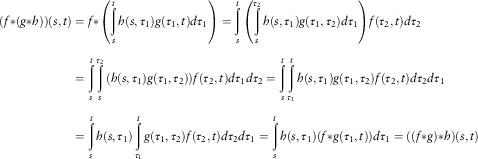 $$\eqalignno{ (f{\asterisk}(g{\asterisk}h))(s,t) & =f{\asterisk}\left( {\mathop{\int}\limits_s^t {h(s,\tau _{1} )g(\tau _{1} ,t)d\tau _{1} } } \right)=\mathop{\int}\limits_s^t {\left( {\mathop{\int}\limits_s^{\tau _{2} } {h(s,\tau _{1} )g(\tau _{1} ,\tau _{2} )d\tau _{1} } } \right)f(\tau _{2} ,t)d\tau _{2} } \cr =\mathop{\int}\limits_s^t {\mathop{\int}\limits_s^{\tau _{2} } {(h(s,\tau _{1} )g(\tau _{1} ,\tau _{2} )} )f(\tau _{2} ,t)d\tau _{1} d\tau _{2} } =\mathop{\int}\limits_s^t {\mathop{\int}\limits_{\tau _{1} }^t {h(s,\tau _{1} )g(\tau _{1} ,\tau _{2} )} f(\tau _{2} ,t)d\tau _{2} d\tau _{1} } \cr =\mathop{\int}\limits_s^t {h(s,\tau _{1} )\mathop{\int}\limits_{\tau _{1} }^t {g(\tau _{1} ,\tau _{2} )f(\tau _{2} ,t)} d\tau _{2} d\tau _{1} } =\mathop{\int}\limits_s^t {h(s,\tau _{1} )(f{\asterisk}g(\tau _{1} ,t))d\tau _{1} } =((f{\asterisk}g){\asterisk}h)(s,t)\,\,\,\,\,\,\,\,\,\,\,\,\,\,\,\,\,\,\,\,\,\,\,\,\,\,\,\,\,\,\,\,\,\,\,\,\,\,\,\,\,\,\,\,\,\,\, $$
Remark 2.1. The fourth step of the proof is the application of Dirichelet’s formula.
Distributivity: given  $f(s,t),\,g(s,t),h(s,t)$
it results that
$f(s,t),\,g(s,t),h(s,t)$
it results that
 $$(f{\asterisk}(g{\plus}h))(s,t)=(f{\asterisk}g)(s,t){\plus}(f{\asterisk}h)(s,t).\,{\rm Left} \ {\rm distributivity}$$
 $$((f{\plus}\,g){\asterisk}h)(s,t)=(f{\asterisk}h)(s,t){\plus}\,(g{\asterisk}h)(s,t).\,{\rm Right \ distributivity}$$
Proof: Indeed, it results:
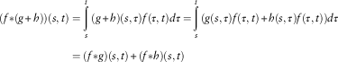 $$\eqalignno{ \qquad(f{\asterisk}(g{\plus}h))(s,t) & =\mathop{\int}\limits_s^t {(g{\plus}h)(s,\tau )f(\tau ,t)d\tau =} \mathop{\int}\limits_s^t {(g(s,\tau )f(\tau ,t){\plus}h(s,\tau )f(\tau ,t))d\tau } \cr & =(f{\asterisk}g)(s,t){\plus}(f{\asterisk}h)(s,t)\,\,\,\,\,\,\,\,\,\,\,\,\,\,\,\,\,\,\,\,\,\,\,\,\,\,\,\,\,\,\,\,\,\,\,\,\,\,\,\,\,\,\,\,\,\,\,\,\,\,\,\,\,\,\,\,\,\,\,\,\,\,\,\,\,\,\,\,\,\,\,\,\,\,\,\,\,\,\,\,\,\,\,\,\,\,\,\,\,\,\,\,\,\,\,\,\,\,\,\,\,\,\,\,\,\,\,\,\,\,\,\,\,\,\,\,\,\,\,\,\,\,\,\,\,\,\,\,\,\,\,\,\,\,\,\,\,\,\,\,\,\,\,\,\,\,\,\,\,\,\,\,\,\,\, $$
Bi-linearity: The additivity is ensured by the distributivity. It remains to be proven that  $\forall a\in {\Bbb R},\,\,\forall f(s,t),\,g(s,t)$
it results:
$\forall a\in {\Bbb R},\,\,\forall f(s,t),\,g(s,t)$
it results:
 $$(a(f{\asterisk}\,g))(s,t)=((af){\asterisk}\,g)(s,t)=(f{\asterisk}\,(ag))(s,t)$$
Proof:
 $$\eqalignno{ & (a(f{\asterisk}g)(s,t))=a\mathop{\int}\limits_s^t {g(s,\tau )f(\tau ,t)d\tau } =\mathop{\int}\limits_s^t {g(s,\tau )af(\tau ,t)d\tau } =((af){\asterisk}\,g)(s,t) \cr & a\mathop{\int}\limits_s^t {g(s,\tau )f(\tau ,t)d\tau } =\mathop{\int}\limits_s^t {ag(s,\tau )f(\tau ,t)d\tau } =(f{\asterisk}(a\,g))(s,t)\,\,\,\,\,\,\,\,\,\,\,\,\,\,\,\,\,\,\,\,\,\,\,\,\,\,\,\,\,\,\,\,\,\,\,\,\,\,\,\,\,\,\,\,\,\,\,\,\,\,\,\,\,\,\,\,\,\,\,\,\,\,\,\,\,\,\,\,\,\,\,\,\,\,\,\,\,\,\,\,\,\,\,\,\, $$
Remark 2.2. The non-homogeneous convolution is non-commutative, i.e.:
 $$\exists f(s,t),g(s,t):\,\,(f{\asterisk}g)(s,t)\,\ne\,(g{\asterisk}f)(s,t)$$
Example 2.1.  $f(s,t)={\rm e}^{{3s{\plus}4t}} ,g(s,t)={\rm e}^{{{ - }4s{\plus}2t}} $
and their convolution is not commutative.
$f(s,t)={\rm e}^{{3s{\plus}4t}} ,g(s,t)={\rm e}^{{{ - }4s{\plus}2t}} $
and their convolution is not commutative.
Remark 2.3. Time homogeneity is a particular case of non-homogeneity. Indeed, a two-time variables case  $f(s,t),\,0\leq s\leq t$
is homogeneous if
$f(s,t),\,0\leq s\leq t$
is homogeneous if
 $$f(s,t)=f(s{\plus}h,t{\plus}h);\,\,\forall 0\leq s\leq t\,\,{\rm and}\,\,h:{ - }s\lt h$$
Given this hypothesis, it is possible to define another one-time variable function
 $$\bar{f}(\tau )=f(s,t),\,\,\,\forall s,t\,{\rm and}\,\,\tau =t{ - }s$$
It results that  $\bar{f}$
is a function of the duration and not of the starting and arriving times.
$\bar{f}$
is a function of the duration and not of the starting and arriving times.
Remark 2.4. Given f and g, the function of two-time variables that are homogeneous in time. Let
 $$\bar{f}(r)=f(t{ - }s)\,\,{\rm and}\,\,\bar{g}(r)=g(t{ - }s),{\rm where}\,\,r=t{ - }s$$
then from the homogeneity hypothesis and posed  $\tau { - }s=x$
it results:
$\tau { - }s=x$
it results:
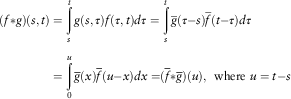 $$\eqalignno{ (f{\asterisk}g)(s,t) & =\mathop{\int}\limits_s^t {g(s,\tau )f(\tau ,t)d\tau } =\mathop{\int}\limits_s^t {\bar{g}(\tau { - }s)\bar{f}(t{ - }\tau )d\tau } \cr =\mathop{\int}\limits_0^u {\bar{g}(x)\bar{f}(u{ - }x)dx=} (\bar{f}{\asterisk}\bar{g})(u),\,\,\,{\rm where } \ u=t{ - }s $$
3. Main Definitions
In this part, the main definitions of the renewal theory, as given in Janssen & Manca (Reference Janssen and Manca2006), are reported in homogeneous and non-homogeneous environments. Let  $$\left( {X_{n} ,\zrLarrnn n \in {\Bbb N}{ - }\left\{ 0 \right\}} \right)$$
be a sequence of positive iid r.v.s in the homogeneous case. In the non-homogeneous case the inter-arrival r.v.s
$$\left( {X_{n} ,\zrLarrnn n \in {\Bbb N}{ - }\left\{ 0 \right\}} \right)$$
be a sequence of positive iid r.v.s in the homogeneous case. In the non-homogeneous case the inter-arrival r.v.s  $X_{n} $
are conditionally independent, in addition, the not necessarily identically distributed r.v.s defined on the probability space
$X_{n} $
are conditionally independent, in addition, the not necessarily identically distributed r.v.s defined on the probability space  $$\left( {\Omega ,F,P} \right)$$
and
$$\left( {\Omega ,F,P} \right)$$
and  ${\Bbb N}$
compose the set of natural numbers.
${\Bbb N}$
compose the set of natural numbers.
Definition 3.1. The random sequence  $$\left( {T_{n} ,\,\,n\geq 0} \right)$$
, where:
$$\left( {T_{n} ,\,\,n\geq 0} \right)$$
, where:
 $$T_{0} =0, \ {\rm and} \ T_{n} =X_{1} {\plus} \cdots {\plus}X_{n} ,\quad n\geq 1$$
is called a generalised renewal sequence or sometimes a general renewal process.
The r.v.s  $$T_{n} ,\,\,n\geq 0$$
are called renewal times. To avoid triviality it is supposed that
$$T_{n} ,\,\,n\geq 0$$
are called renewal times. To avoid triviality it is supposed that  $P\left[ {X_{n} \leq 0=0} \right].$
Definition 3.2. The random sequence  $$\left( {T_{n} ,\,\,n\geq 0} \right)$$
is a homogeneous classical renewal process if the
$$\left( {T_{n} ,\,\,n\geq 0} \right)$$
is a homogeneous classical renewal process if the  $X_{n} ,n\geq 1$
r.v.s are identically distributed and independent with F as d.f.
$X_{n} ,n\geq 1$
r.v.s are identically distributed and independent with F as d.f.
Definition 3.3. The random sequence $$\left( {T_{n} ,\,\,n\geq 0} \right)$$
is a non-homogeneous classical renewal process if variables
$$\left( {T_{n} ,\,\,n\geq 0} \right)$$
is a non-homogeneous classical renewal process if variables  $X_{n} ,n\geq 1$
are conditionally independent and non-identically defined (see Dawid, Reference Dawid1979). Given
$X_{n} ,n\geq 1$
are conditionally independent and non-identically defined (see Dawid, Reference Dawid1979). Given
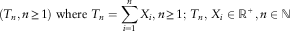 $$(T_{n} ,n\geq 1) \ {\rm where } \ T_{n} =\mathop{\sum}\limits_{i=1}^n {X_{i} } ,n\geq 1;\,T_{n} ,\,X_{i} \in {\Bbb R}^{{\plus}} ,n\in {\Bbb N}$$
and the function F is the conditional d.f. of  $$X_{n} $$
given
$$X_{n} $$
given  $$T_{n} $$
defined as follows:
$$T_{n} $$
defined as follows:
 $$F(s,t)=P(X_{n} \leq t{ - }s\left| {T_{{n{ - }1}} } \right.=s),0\lt s\leq t$$
And for  $s=0$
, we have:
$s=0$
, we have:
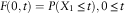 $$F(0,t)=P(X_{1} \leq t),0\leq t$$
It follows that the process  $$(T_{n} ,n\geq 0)$$
is a non-homogeneous Markov process with one state and values in
$$(T_{n} ,n\geq 0)$$
is a non-homogeneous Markov process with one state and values in  $${\Bbb R}^{{\plus}} $$
.
$${\Bbb R}^{{\plus}} $$
.
Remark 3.1. In delayed homogeneous renewal processes,  $X_{1} $
has a different distribution with respect to
$X_{1} $
has a different distribution with respect to  $X_{n} ,\,n\geq 2$
.
$X_{n} ,\,n\geq 2$
.
Definition 3.4. With each renewal sequence, the following stochastic process can be associated with values in  $${\Bbb N}$$
:
$${\Bbb N}$$
:
 $$\left( {N(t),\zrLarr\zrLarr\zrLarrt t \in {\Bbb R}^{{\plus}} } \right)$$
 $$N(t)$$
represents the total number of “renewals” on
$$N(t)$$
represents the total number of “renewals” on  $$(0,t]$$
and in the homogeneous and non-homogeneous cases, it respectively results:
$$(0,t]$$
and in the homogeneous and non-homogeneous cases, it respectively results:
 $$\eqalignno{ & N(t)\,\gt \,n { - }1 \Leftrightarrow T_{n} \leq t,\quad \quad n\in {\Bbb N} \cr & N(t){ - }N(s)\gt n{ - }1\Leftrightarrow T_{{n'}} =s,T_{{n\Prime}} \leq t,\,\,n\Prime { - }n\prime \gt n{ - }1\,\, \cr & s\in {\Bbb R}_{0}^{{\plus}} ,t\in {\Bbb R}^{{\plus}} ;n,n',n\quote\in {\Bbb N} $$
These processes are, respectively, called the homogeneous and non-homogeneous associated counting process or the homogeneous and non-homogeneous renewal counting process.
Remark 3.2. The probabilities of having at least n renewals within a time t in the homogeneous case given (2) and from time s to time t in the non-homogeneous environment given (3) and (4) are, respectively, given by:
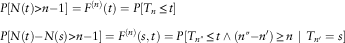 $$\eqalignno{ & P\left[ {N(t)\gt n{ - }1} \right]=F^{{(n)}} (t)=P[T_{n} \leq t] \cr & P\left[ {N(t){ - }N(s)\gt n{ - }1} \right]=F^{{(n)}} (s,t)=P[T_{{n{\rm \Prime}}} \leq t\wedge(n{\rm \Prime}{ - }n')\geq n\,\mid\,T_{{n'}} =s] $$
The probabilities of having just n renewals are obtained in the following way:
 $$P\left[ {N(t)=n} \right]=P\left[ {N(t)\gt n{ - }1} \right]{ - }P\left[ {N(t)\gt n} \right]=F^{{(n)}} (t){ - }F^{{(n{\plus}1)}} (t)$$
 $$\eqalignno{ & P\left[ {N(t){ - }N(s)=n} \right]=P\left[ {N(t){ - }N(s)\gt n{ - }1} \right] \cr & { - }P\left[ {N(t){ - }N(s)\gt n} \right]=F^{{(n)}} (s,t){ - }F^{{(n{\plus}1)}} (s,t) $$
Furthermore, it results:
 $$F(s,t)=P[T_{{n{\rm \Prime}}} \leq t\wedge(n{\rm \Prime}{ - }n')\geq 1\,\mid\,T_{{n'}} =s]$$
and by conditional independence it is obtained:
 $$F^{{(2)}} (s,t)=P[T_{{n{\rm \Prime}}} \leq t\wedge(n{\rm \Prime}{ - }n')\geq 2\,\mid\,T_{{n'}} =s]$$
Iterating the last relation the relation (7) is obtained in the non-homogeneous case.
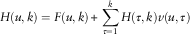
Definition 3.5. The homogeneous and non-homogeneous renewal functions are defined, respectively, as:
 $$\eqalignno{ & H(t)=E\left[ {N(t)} \right],\,\,\,0\leq t,\,\,t\in {\Bbb R}_{0}^{{\plus}} \cr & H(s,t)=E\left[ {N(t){ - }N(s)} \right]{\rm =}E\left[ {N(t)} \right]{ - }E\left[ {N(s)} \right],\,\,0\leq s\leq t\,\,\,s,t\in {\Bbb R}_{0}^{{\plus}} $$
provided that the expectation is finite. They give the mean number of renewals verified within a time t and from time s to time t, respectively.
Definition 3.6. Given two non-homogeneous distribution functions (n.h.d.f) F(s,t) and G(s,t), their convolution operation is defined in the following way:
 $$G{\asterisk}F(s,t)=\mathop{\int}\limits_s^t {G(\tau ,t)dF(s,\tau )} $$
Proposition 3.1. The homogeneous and non-homogeneous continuous time evolution equation of the renewal equations, supposing the absolute continuity of the d.f. F, i.e.,  $dF(t)=f(t)dt$
, can be written, respectively, in the following way:
$dF(t)=f(t)dt$
, can be written, respectively, in the following way:
 $$\eqalignno{ & H(t)=F(t){\plus}\mathop{\int}\limits_0^t {f(\tau )H(t{ - }\tau )d\tau } \cr & H(s,t)=F(s,t){\plus}\mathop{\int}\limits_s^t {f(s,\tau )H(\tau ,t)d\tau } $$
Proof: For the homogeneous case see, for example, Janssen & Manca (Reference Janssen and Manca2006).
In the non-homogeneous case it results:
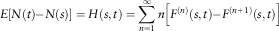 $$E\left[ {N(t){ - }N(s)} \right]=H(s,t)=\mathop{\sum}\limits_{n=1}^\infty {n\left[ {F^{{(n)}} (s,t){ - }F^{{(n{\plus}1)}} (s,t)} \right]} $$
 $$\eqalignno{ & H(s,t)=\mathop{\sum}\limits_{n=1}^\infty {F^{{(n)}} (s,t)} =F(s,t){\plus}\mathop{\sum}\limits_{n=2}^\infty {F^{{(n)}} (s,t)} \cr & =F(s,t){\plus}\left( {\mathop{\sum}\limits_{n=2}^\infty {F^{{(n{ - }1)}} } } \right){\asterisk}F(s,t)=F(s,t){\plus}\left( {\mathop{\sum}\limits_{n=1}^\infty {F^{{(n)}} } } \right){\asterisk}F(s,t) \cr & H(s,t)=F(s,t){\plus}H{\asterisk}F(s,t) $$
 $$H(s,t)=F(s,t){\plus}\mathop{\int}\limits_s^t {f(s,\tau )H(\tau ,t)d\tau } $$
Definition 3.7. The homogeneous and non-homogeneous discrete time evolution equations of the renewal processes are, respectively, as follows:
 $$\eqalignno{ & H(t)=F(t){\plus}\mathop{\sum}\limits_{\tau =1}^t {\nu (\tau )H(t{ - }\tau )} ;\,\,t\in {\Bbb N}{ - }\left\{ 0 \right\} \cr & H(s,t)=F(s,t){\plus}\mathop{\sum}\limits_{\tau =s{\plus}1}^t {\nu (s,\tau )H(\tau ,t)} ;s\in {\Bbb N},\,t\in {\Bbb N}{ - }\left\{ 0 \right\} $$
where  $F(t)\,{\rm and}\,F(s,t)$
are the respective waiting times d.f.s for the discrete time homogeneous and non-homogeneous d.f. They give the probability of having a renewal within the time t in the homogeneous case, and also the probability to have a renewal within the time t given that the previous renewal happened just at time s in the non-homogeneous environment.
$F(t)\,{\rm and}\,F(s,t)$
are the respective waiting times d.f.s for the discrete time homogeneous and non-homogeneous d.f. They give the probability of having a renewal within the time t in the homogeneous case, and also the probability to have a renewal within the time t given that the previous renewal happened just at time s in the non-homogeneous environment.  $H(t)\,{\rm and}\,H(s,t)$
, in this case, respectively, represent the discrete time homogeneous and non-homogeneous renewal equations, i.e., the mean number of renewals, respectively, within the time t in the homogeneous and from time s within the time t in the non-homogeneous environments. Furthermore, it results that:
$H(t)\,{\rm and}\,H(s,t)$
, in this case, respectively, represent the discrete time homogeneous and non-homogeneous renewal equations, i.e., the mean number of renewals, respectively, within the time t in the homogeneous and from time s within the time t in the non-homogeneous environments. Furthermore, it results that:
 $$\eqalignno{ & \nu (t)=\left\{ {\matrix{ 0 & {{\rm if}} & {t=0} \cr {F(t){ - }F(t{ - }1)} & {{\rm if}} & {t\gt 0} \cr } } \right. \cr & $$
and
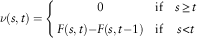 $$\nu (s,t)=\left\{ {\matrix{ 0 & {{\rm if}} & {s\geq t} \cr {F(s,t){ - }F(s,t{ - }1)} & {{\rm if}} & {s\lt t} \cr } } \right.$$
Remark 3.3. In the homogeneous case, the definitions of continuous and discrete time evolution equations correspond to those given, respectively, in Feller (Reference Feller1971: 185) and Feller (Reference Feller1968: 332).
4. Solving the Non-Homogeneous Discrete Time Evolution Equation
The discrete time non-homogeneous renewal equation (10) can be numerically solved very easily (for the homogeneous case see Janssen & Manca, Reference Janssen and Manca2006). Compactly expressed, the non-homogeneous case of relation (10) can be written as:
 $$H(s,t){ - }\mathop{\sum}\limits_{\tau =s{\plus}1}^t {\nu (s,\tau )H(\tau ,t)} =F(s,t)\Leftrightarrow{\bf U} \cdot {\bf H}={\bf F}$$
where:
 $${\bf U}=\left[ {\matrix{ 1 & {{ - }v(0,1)} & \cdots & {{ - }v(0,k)} & \cdots & {{ - }v(0,n)} \cr 0 & 1 & \cdots & {{ - }v(1,k)} & \cdots & {{ - }v(1,n)} \cr \vdots & \vdots & \ddots & \vdots & \ddots & \vdots \cr 0 & 0 & \cdots & 1 & \cdots & {{ - }v(k,n)} \cr \vdots & \vdots & \ddots & \vdots & \ddots & \vdots \cr {\matrix{ 0 \cr \vdots \cr } } & {\matrix{ 0 \cr \vdots \cr } } & {\matrix{ \cdots \cr \ddots \cr } } & {\matrix{ 0 \cr \vdots \cr } } & {\matrix{ \cdots \cr \ddots \cr } } & {\matrix{ 1 \cr \vdots \cr } } \cr } \matrix{ \cdots \cr \cdots \cr \ddots \cr \cdots \cr \ddots \cr {\matrix{ \cdots \cr \ddots \cr } } \cr } } \right]$$
is the coefficient matrix;
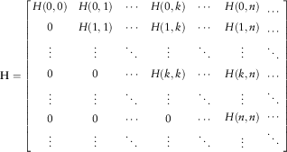 $${\bf H}=\left[ {\matrix{ {H(0,0)} & {H(0,1)} & \cdots & {H(0,k)} & \cdots & {H(0,n)} \cr 0 & {H(1,1)} & \cdots & {H(1,k)} & \cdots & {H(1,n)} \cr \vdots & \vdots & \ddots & \vdots & \ddots & \vdots \cr 0 & 0 & \cdots & {H(k,k)} & \cdots & {H(k,n)} \cr \vdots & \vdots & \ddots & \vdots & \ddots & \vdots \cr {\matrix{ 0 \cr \vdots \cr } } & {\matrix{ 0 \cr \vdots \cr } } & {\matrix{ \cdots \cr \ddots \cr } } & {\matrix{ 0 \cr \vdots \cr } } & {\matrix{ \cdots \cr \ddots \cr } } & {\matrix{ {H(n,n)} \cr \vdots \cr } } \cr } \matrix{ \cdots \cr \cdots \cr \ddots \cr \cdots \cr \ddots \cr {\matrix{ \cdots \cr \ddots \cr } } \cr } } \right]$$
is the unknown matrix and
 $${\bf F}=\left[ {\matrix{ {F(0,0)} & {F(0,1)} & \cdots & {F(0,k)} & \cdots & {F(0,n)} \cr 0 & {F(1,1)} & \cdots & {F(1,k)} & \cdots & {F(1,n)} \cr \vdots & \vdots & \ddots & \vdots & \ddots & \vdots \cr 0 & 0 & \cdots & {F(k,k)} & \cdots & {F(k,n)} \cr \vdots & \vdots & \ddots & \vdots & \ddots & \vdots \cr {\matrix{ 0 \cr \vdots \cr } } & {\matrix{ 0 \cr \vdots \cr } } & {\matrix{ \cdots \cr \ddots \cr } } & {\matrix{ 0 \cr \vdots \cr } } & {\matrix{ \cdots \cr \ddots \cr } } & {\matrix{ {F(n,n)} \cr \vdots \cr } } \cr } \matrix{ \cdots \cr \cdots \cr \ddots \cr \cdots \cr \ddots \cr {\matrix{ \cdots \cr \ddots \cr } } \cr } } \right]$$
is the matrix in which each row is a discrete time d.f.
Remark 4.1. System (11) allows for the solution. Indeed, the determinant of the coefficient matrix of the system (11) is equal to 1 (see Riesz, Reference Riesz1913).
Remark 4.2.  $F(k,k)=0$
because it is impossible to have a renewal in a time 0. This implies
$F(k,k)=0$
because it is impossible to have a renewal in a time 0. This implies  $v(k,k)=0$
and
$v(k,k)=0$
and  $H(k,k)=0$
.
$H(k,k)=0$
.
4.1. Some particular formulae
In this part, some formulas of the numerical solution of the non-homogeneous part of the renewal equations in (9) will be given. The relations will be related to particular generalised Newton–Cotes formulas (see Hildebrand, Reference Hildebrand1987).
The Simpson quadrature method gives the following equations:
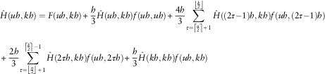 $$\eqalignno{ & \hat{H}(uh,kh)=F(uh,kh){\plus}{h \over 3}\hat{H}(uh,kh)f(uh,uh){\plus}{{4h} \over 3}\mathop{\sum}\limits_{\tau =\left\lceil {{u \over 2}} \right\rceil {\plus}1}^{\left\lfloor {{k \over 2}} \right\rfloor } {\hat{H}\left( {(2\tau { - }1)h,kh} \right)f\left( {uh,(2\tau { - }1)h} \right)} \cr & \zrLarr\zrLarr\zrLarr\zrLarr\zrLarr\zrLarr\zrLarr\zrLarr\zrLarr\zrLarr\zrLarr\zrLarr\zrLarr\zrLarr\zrLarr\zrLarr\zrLarr\zrLarr\zrLarr\zrLarr\zrLarr\zrLarr\zrLarr{\plus}{{2h} \over 3}\mathop{\sum}\limits_{\tau =\left\lfloor {{u \over 2}} \right\rfloor {\plus}1}^{\left\lceil {{k \over 2}} \right\rceil { - }1} {\hat{H}\left( {2\tau h,kh} \right)f\left( {uh,2\tau h} \right)} {\plus}{h \over 3}\hat{H}(kh,kh)f(uh,kh) $$
where  $\hat{H}$
represents the approximate value of H and h the discretisation interval.
$\hat{H}$
represents the approximate value of H and h the discretisation interval.
Using Bezout’s quadrature method, the following relation is obtained:
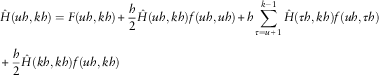 $$\eqalignno{ & \hat{H}(uh,kh)=F(uh,kh){\plus}{h \over 2}\hat{H}(uh,kh)f(uh,uh){\plus}h\mathop{\sum}\limits_{\tau =u{\plus}1}^{k{ - }1} {\hat{H}\left( {\tau h,kh} \right)f\left( {uh,\tau h} \right)} \cr & \zrLarr\zrLarr\zrLarr\zrLarr\zrLarr\zrLarr\zrLarr\zrLarr\zrLarr\zrLarr\zrLarr\zrLarr\zrLarr\zrLarr\zrLarr\zrLarr\zrLarr\zrLarr\zrLarr\zrLarr\zrLarr\zrLarr\zrLarr{\plus}{h \over 2}\hat{H}(kh,kh)f(uh,kh) $$
Finally, if the simplest quadrature method (rectangle formula) is applied, then it is possible to obtain two different formulas: one giving the value of the integrating function at the end of the interval and the other at the beginning of the interval. In this way, the following formulas are obtained:
 $$\hat{H}(uh,kh)=F(uh,kh){\plus}h\!\!\!\mathop{\sum}\limits_{\tau =u{\plus}1}^k {\hat{H}\left( {\tau h,kh} \right)f\left( {uh,\tau h} \right)} $$
 $$\hat{H}(uh,kh)=F(uh,kh){\plus}h\mathop{\sum}\limits_{\tau =u}^{k{ - }1} {\hat{H}\left( {\tau h,kh} \right)f\left( {uh,\tau h} \right)} $$
Substituting the differential  $(hf(uh,kh))$
by means of the difference, it, respectively, results:
$(hf(uh,kh))$
by means of the difference, it, respectively, results:
 $$\eqalignno{ & \hat{H}(uh,kh)\,\cong\,F(uh,kh){\plus}\mathop{\sum}\limits_{\tau =u{\plus}1}^k {\hat{H}\left( {\tau h,kh} \right)\left( {F\left( {uh,\tau h} \right){ - }F(uh,(\tau { - }1)h)} \right)} \cr & \hat{H}(uh,kh)\,\cong\,F(uh,kh){\plus}\mathop{\sum}\limits_{\tau =u}^{k{ - }1} {\hat{H}\left( {\tau h,kh} \right)\left( {F\left( {uh,(\tau {\plus}1)h} \right){ - }F(uh,(\tau )h)} \right)} $$
Remark 4.3. In Baker (Reference Baker1977: 925), there are two lemmas and a theorem ensuring that, under our conditions, the error approximation of (12) to the solution tends to 0, as the discretisation interval h tends to 0. However, in the following and given our particular system, we are able to give a more interesting result.
4.2. Relations between discrete time and continuous time-renewal equations
Posing h=1 in (12):
 $$\hat{H}(u,k)\,\cong\,F(u,k){\plus}\mathop{\sum}\limits_{\tau =u{\plus}1}^k {\hat{H}\left( {\tau ,k} \right)\left( {F\left( {u,\tau } \right){ - }F(u,\tau { - }1)} \right)} $$
Furthermore, giving the following positions:
 $$v(u,\tau )=\left\{ {\matrix{ {F(u,\tau )=0} & {\tau =u} \cr {F(u,\tau ){ - }F(u,\tau { - }1)} & {\tau \gt u} \cr } } \right.$$
the following is obtained:
 $$H(u,k)=F(u,k){\plus}\mathop{\sum}\limits_{\tau =1}^k {H\left( {\tau ,k} \right)v(u,\tau )} $$
that is the discrete time non-homogeneous renewal equation.
Now let H be a continuous time-renewal function and {T n} the related renewal process.
If the following is set:
 $$T_{n}^{h} =\left\lfloor {{{T_{n} } \over h}} \right\rfloor h$$
and
 $$N^{h} (t)=n\,{\rm if}\;T_{n}^{h} \leq t\lt T_{{n{\plus}1}}^{h} $$
then the related discrete time-renewal function is given by:
 $$H^{h} (uh,kh)=F^{h} (uh,kh)\!{\plus}\!\!\mathop{\sum}\limits_{\tau =u{\plus}1}^k {v^{h} (uh,\tau h)H^{h} \left( {(k{ - }\tau )h,kh} \right)} $$
The renewal process  $T_{n}^{h} $
is defined in the same probability space
$T_{n}^{h} $
is defined in the same probability space  $$\left( {\Omega ,F,P} \right)$$
of T n.
$$\left( {\Omega ,F,P} \right)$$
of T n.
Given  $$\omega \in \Omega $$
the following result holds:
$$\omega \in \Omega $$
the following result holds:
Proposition 4.1. The  $T_{n}^{h} $
process converges to T nfor
$T_{n}^{h} $
process converges to T nfor  $$h\to0$$
.
$$h\to0$$
.
Proof: From the definitions given in section 3 and (14) it results:
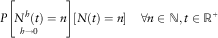 $$P\left[ {\mathop{{N^{h} (t)}}\limits_{{h\to0}} =n} \right]\toP\left[ {N(t)=n} \right]\,\,\,\,\,\,\,\forall n\in {\Bbb N},t\in {\Bbb R}^{{\plus}} $$
The formula (15) implies:
 $$\mathop{{T_{n}^{h} }}\limits_{{h\to0}} \buildrel {a.s.} \over \longrightarrow T_{n} $$
Remark 4.4. The Proposition 4.1 can be considered a very special case of the Theorem 10 that is given in Janssen & Manca (Reference Janssen and Manca2001). However, in this paper, the proof is trivial. Indeed, if  $h\to0$
and being the rational set dense in
$h\to0$
and being the rational set dense in  ${\Bbb R}$
it results in the intuitive understanding of relation (15).
${\Bbb R}$
it results in the intuitive understanding of relation (15).
Remark 4.5. The results obtained show that it is possible to obtain the non-homogeneous discrete time-renewal equation by means of the simplest discretisation of the related continuous time and that, starting from the discrete time, it is also possible to obtain the continuous time.
Remark 4.6. Freiberger & Grenander (Reference Freiberger and Grenander1971) demonstrate a similar approach to obtaining the renewal equation numerical solution for the homogeneous case, but there is no justification of the method. Many other papers (see section 1) deal with the same problem in the homogeneous case, but, as far as the authors are aware, the relationship between the discrete time and continuous time-renewal process has only been justified in the book by Janssen & Manca (Reference Janssen and Manca2006), as they are in this paper in the non-homogeneous case. It is, however, the first time that the numerical treatment of the non-homogeneous renewal processes is presented.
5. Car Insurance Mean Number Claims Calculation in a Non-Homogeneous Age Environment
5.1. The construction of homogeneous and non-homogeneous d.f.
In this section, we describe the construction of d.f.s from the raw data. We will show, first, the homogeneous case followed by the non-homogeneous case.
Each insured individual corresponds to a record. For each record, the necessary data in the homogeneous case are:
∙ how many accidents the subject caused in the observed time horizon; and
∙ the date of each accident.
The vector of the number of claims that will be paid from the insurance company will be constructed from these data. In ith elements of the vector, there will be the number of accidents that occurred just in i years from the first car insurance contract or from the previous accident. At the end of this process, the vector will have the following shape (Table 1).
Table 1 Number of claims within the time i.
T represents the horizon time and  $T=\max (i)$
where i is the set of all the possible times obtained during the observation of the data. Subsequently, another vector will be created whose elements are defined in the following way:
$T=\max (i)$
where i is the set of all the possible times obtained during the observation of the data. Subsequently, another vector will be created whose elements are defined in the following way:
 $$v(i)=\mathop{\sum}\limits_{k=1}^i {n(k)} $$
The next step will create the d.f., i.e.:
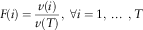 $$F(i)={{v(i)} \over {v(T)}},\,\,\forall i=1,\,\ldots\,,T$$
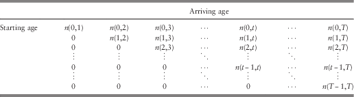
In the non-homogeneous case, a vector will be created for each age s, i.e.:
Remark 5.1 The age 0 corresponds to the starting age 18. The d.f. are constructed for each starting age. At time 0 it is impossible to have a claim, for this reason in the main diagonal of Table 2 there are the ages s−1 and s. The non-homogeneous d.f. F(s,t) should be calculated as  $\forall s=0,\,\ldots\,,T{ - }1$
in the same way as the F(t) in the homogeneous case.
$\forall s=0,\,\ldots\,,T{ - }1$
in the same way as the F(t) in the homogeneous case.
Table 2 Number of claims reported starting from age s just at age t>s.
5.2. The data description
In this section, the non-homogeneous renewal equation is applied to a real actuarial data application, in order to demonstrate that it can be applied in a very general case utilising data from statistical observations. The relation that will be used in this case is (13).
The renewal process will be applied to calculate the mean number of claims; a common problem for motorcar insurance companies. In this insurance, as it is well known, the age of the insured person assumes great relevance. It is possible to take into account the different behaviours of insured people as a function of age by means of a non-homogeneous renewal process where the non-homogeneity is related to age.
In a motorcar insurance contract, each time the insured has an accident the insurance company will pay for the damage. In our model, the renewed contract will consider the driver’s age. Our non-homogeneous environment takes into account this fact. Indeed, the d.f. were different as a function of the starting age, but the independence hypothesis holds.
We have raw data regarding accidents that an insurance company collected during a period of about 50 years up to the year 2000. It is possible to construct the non-homogeneous discrete time d.f. of the renewal time of the motorcar claims from this data. The data covers a total of 156,428 insured people of which 22,395 had at least one accident. Data concerning the insurance premiums, however, were not available. The dates of individual contracts were available and 60,278 of those appeared to be correct. The ages of all the insured people were known. We computed the mean age upon entering the contract of these 60,278 records and found that it was 23.77 years. We supposed that all the other 96,150 insured people entered the contract at age 24. As a result, we had 32,201 claims in total. At most, we had three claims per insured person. For example, the renewal worked in this way; it was supposed that an insured person entered her/his contract at 23 years. She/he made the first claim at 41. We took into account that, for this insured person of starting age 23, there was a claim after 18 years. The renewed age was now 41. It was supposed that she/he made another claim at age 50. In this way, we also supposed that a person that was 41 years old made a new claim after 9 years.
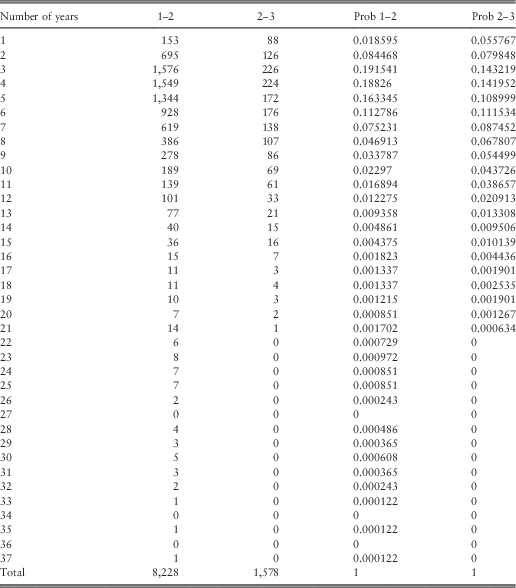
Before applying our model, we did a preliminary study on the data working in a homogeneous environment. To get correct results, we worked on the second and third accidents because, in this way, we were sure about the time of the renewal. The dates of claims were considered to be accurate. The results are reported in Table 3.
Table 3 Homogeneous study of II and III claims.

In this table, the number of accidents reported after 1 year, then after 2 years, and so on, are given in the second and third column. The headings 1–2 means that the number of claims is related to the second accident and that the waiting time is given by the time that passed between the first and the second claim. This waiting time is reported in the first column. The heading of the third column has the same meaning and its contents report the number of claims that occurred at the waiting time given in the first column. For example, 1,576 in the third row of this table represents the number of second accidents that occurred after 2 years and before the 3rd year since the first accident. The number 226 represents the number of third accidents that occurred after 2 years and before the 3rd year since the second accident. The fourth and fifth columns give the probability function of waiting times that are related to columns 2 and 3, respectively.
Figure 1 reports the histograms of the last two columns of Table 3.
Figure 1 Probability distribution obtained by data of the II and III claims.
From the first study of data we know:
1. 14.3% of our population had accidents;
2. <40% of the information is totally reliable.
It is clear from the shape of the histograms that the discrete time probability distribution is not geometric and this implies that our renewal process does not abide by Poisson’s function.
Given that a non-homogeneous model had to be constructed, we decided to take into account all the data related to an accident. To do this, an entrance age of 24 years was given to all those who did not have the correct age upon entering the contract. We did not consider the claims with a date earlier than the starting age of the contract or of the previous renewal. In the end, we considered 23,395 claims and discarded 8,806 accidents.
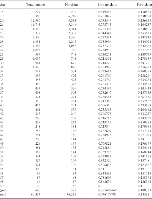
We also constructed a statistic on the 60,278 reliable records of those who did not make claims as a function of their age upon entering the contract. We report these data in Table 4. In these data, which are more reliable than the data of the complete file, a higher probability of having accidents was obtained. The global probability of having an accident becomes 23.3% instead of 9%. Furthermore, we constructed the matrix of occurrences taking into account all the data, i.e., for each starting age from 18 to 60 (after 60 there were fewer new contracts so we compiled them all together), we constructed the number of claims that were made according to the age of the person who caused the accident (see Figure 2). Normalising for each age, we obtained the probability function for each starting age. The shape of the probability function is the same as the shape of occurrences. In addition, in this case it is evident that, as in the homogeneous case, the probability functions do not have the same shape as a geometric probability distribution and the Poisson’s hypotheses should be rejected.
Figure 2 Occurrence distribution of claims as a function of the contract age.
Table 4 Probability of not having claims.
5.3. The result description
In light of these results, we decided to work with the physical measure. We constructed the waiting time probability functions for each starting age from the occurrences. From these probability functions, we constructed the cumulative d.f. and we could then apply the relation (13).
To show just how simple it is to solve the non-homogeneous renewal equation and, subsequently, to obtain the mean number of renewals for each considered age, we report the program written in Mathematica 9 language.
frip=Tables [0.0,{i,1,43},{j,1,43}];
phi=Tables [0.0,{i,1,43},{j,1,43}];
For[i=1,i≤nanni,i++,
frip[[i]]=ReadList [puntf,Number,nanni];
];
For[h=nanni,h≥2,h- -,
For[k=h-1,k≥1,k- -,
phi[[k,h]]=frip[[k,h]];
For[i=k+1, i≤h-1, i++,
phi[[k,h]]+=phi[[i,h]]*(frip[[k,i]]-frip[[k,i-1]]);
];
];
];
In Figure 3, the non-homogeneous d.f. obtained from the data are given.
Figure 3 Waiting time d.f. as a function of age.
Finally, in Table 5, the mean number of claims for starting ages 20–30 and for each age of making a claim is given. The comparison should be done along the diagonal because, in this way, the same number of years is considered.
Table 5 Mean number of claims – starting ages 20–30.
6. Conclusions
In the authors’ opinion, the main results of this paper are:
1. the defining of non-homogeneous in time convolutions and their properties;
2. the systematisation of the theory of non-homogeneous renewal processes;
3. the numerical treatment of non-homogeneous renewal processes;
4. the application of the method to the motorcar insurance environment; and
5. the possibility, within the renewal equation, of using the d.f. constructed directly from the observed data explaining how simple it is to start from the real data and to apply the model.
The proposed application in the field of automobile insurance could be interesting for insurance companies. Indeed, by being able to predict the mean number of claims a person will make on their motorcar insurance contract at a given age during his/her driving life, companies can judge as to whether an insured person is a good or bad driver.
In the near future, we will attempt to also introduce the running time in our model. The construction of such a model will imply that the results will be a function of two-time variables.
Acknowledgements
The authors are grateful to the two anonymous referees, who with their comments improved the paper substantially. The paper was prepared under a grant of “University of Roma La Sapienza”. Work partially supported by MIUR-PRIN and “La Sapienza” grants.