


1. Introduction
It is well known that socio-economic inequalities in death rates and life expectancies exist in many countries. Those inequalities have been documented in the literature, see, for example, Mackenbach et al. (Reference Mackenbach, Kunst, Cavelaars, Groenhof and Geurts1997) and Balia & Jones (Reference Balia and Jones2008).
From an actuarial point of view, it is important to take those differences into account for the pricing of annuities or life insurance products, and this is best achieved by considering stochastic mortality models that aim to capture the dynamics of death rates in different socio-economic groups, while also allowing for common features that are shared by all.
In this paper, we consider socio-economic groups defined with reference to the Index of Multiple Deprivation (IMD) in England. This index measures relative deprivation and allows us to identify 10 groups. A brief empirical study of those 10 groups can be found in Kleinow et al. (Reference Kleinow, Cairns and Wen2019).
In recent years, a number of approaches have been developed to model socio-economic differences in mortality rates. Villegas & Haberman (Reference Villegas and Haberman2014) fitted extended versions of the Lee–Carter model to socio-economic sub-populations in England. Bennett et al. (Reference Bennett, Li, Foreman, Best, Kontis, Pearson, Hambly and Ezzati2015) discussed modelling life expectancies in different areas of England and Wales via a Baysian model with spatial effects. They found significant differences in life expectancy and also the pace of improvements in life expectancy between different areas of England and Wales. Cairns et al. (Reference Cairns, Kallestrup-Lamb, Rosenskjold, Blake and Dowd2019) identify different socio-economic groups and model their mortality rates using an affluence index rather than the IMD used in this paper. Closer to the approach in this paper is our study in Wen et al. (2020) where we fit multi-population models to distinct groups of members of the Canada Pension Plan (CPP) and the Quebec Pension Plan (QPP). In that study, we found significant differences between groups in terms of mortality levels and pace of mortality improvements.
The main question we aim to answer in this paper is what model should be fitted to the group-specific data keeping in mind that all groups are sub-populations of the English national population, which suggests that they might share some common characteristics. Therefore, we are looking for a stochastic mortality model for multiple populations that allows us to capture common features as well as group-specific factors.
Many stochastic multi-population models for mortality have been proposed in the literature. The most well-known model is that suggested by Li & Lee (Reference Li and Lee2005). Their model is an extension of the Lee–Carter model, Lee & Carter (Reference Lee and Carter1992), that combines common age and time trends affecting all populations with population-specific components to allow for derivations from the common mortality table. An alternative is the CAE model suggested by Kleinow (Reference Kleinow2015). This model is also a modification of the Lee–Carter model. But, in contrast to the Li and Lee model, the CAE model treats all or some age effects as common, while allowing for population-specific period effects.
Some models that were originally developed for a single population can easily be adapted to multiple populations by allowing for some parameters to be common to all of them. One example is the model proposed by Plat (Reference Plat2009) which is one of the models that we adapt to fit multiple populations.
To be more specific, the contribution of this paper is a quantitative comparison of a number of stochastic multi-population models fitted to the mortality experiences in 10 socio-economic groups in England. We introduce the different models and first compare them using the Bayesian Information Criterion (BIC). We then take a closer look at the best preforming models discussing the parameter estimates obtained for those models with a focus on identifying those parameters that capture the differences between groups and parameters that are common to all groups.
We also compare the fitted model-specific death rates with those actually observed in the 10 groups to get a better idea of the advantages and shortcomings of the different models. While we will mostly focus on data for the female population, we find that models with cohort effects perform well for the male population, and we therefore investigate those in more detail for both sexes.
While we concentrate in this paper on quantitative measures and goodness of fit for model selection, we should mention that other model properties, often called qualitative criteria, are also important to consider when models are chosen for a particular application: see section 3.4 for further details. For example, models that result in perfect correlation between mortality improvements in different groups are not a good choice as they ignore group-specific trends. There are, of course, a number of other considerations, see, for example, Villegas et al. (Reference Villegas, Haberman, Kaishev and Millossovich2017) and Wen et al. (2020), and we will mention some of those when we discuss individual models. However, the focus of this paper is on quantitative criteria.
The remainder of the paper is organised as follows. We first describe the available data and discuss some empirical findings in section 2. In section 3, we then introduce the set of mortality models which we fit to the available data, and we then provide a first quantitative comparison of models in terms of their BIC in section 4. Parameter estimates for some selected models are presented in section 5, and the fitted death rates implied by different models are discussed in section 6. In this section, we find that some models might benefit from the inclusion of a cohort effect which we investigate in section 7. Finally, we summarise our main conclusions in section 8.
2. The Data
The data for our study consist of sex-specific deaths counts and exposures for 10 socio-economic groups in England. The groups are determined by the IMD published by the UK Office for National Statistics (ONS). In the following, we provide a brief description of the IMD and the related mortality data.
2.1 Index of multiple deprivation
The ONS measures different aspects of deprivation in small geographic areas in England, called Lower Layer Super Output Areas (LSOAs). All LSOAs are of similar population size dividing the entire population into 32,844 small groups. The IMD is then calculated for each LSOA as a weighted average of seven indices measuring different aspects of deprivation: income (weight
 $22.5\%$
), employment (
$22.5\%$
), employment (
 $22.5\%$
), education (
$22.5\%$
), education (
 $13.5\%$
), crime (
$13.5\%$
), crime (
 $9.3\%$
), health (
$9.3\%$
), health (
 $13.5\%$
), barriers to housing and services (
$13.5\%$
), barriers to housing and services (
 $9.3\%$
), and living environment (
$9.3\%$
), and living environment (
 $9.3\%$
). Each of those seven indices is based on a basket of indicators from the most recently available statistics. The IMD score for an individual LSOA represents a measure for the relative deprivation of the population living in that LSOA compared to other LSOAs. The LSOAs are then ranked according to their IMD score from the most deprived to the least deprived area in England and 10 deciles are formed. Detailed information about the IMD can be found in Smith et al. (Reference Smith, Noble, Noble, Wright, McLennan and Plunkett2015a) and (Reference Smith, Noble, Noble, Wright, McLennan and Plunkett2015b) where the construction of the index is explained in detail.
$9.3\%$
). Each of those seven indices is based on a basket of indicators from the most recently available statistics. The IMD score for an individual LSOA represents a measure for the relative deprivation of the population living in that LSOA compared to other LSOAs. The LSOAs are then ranked according to their IMD score from the most deprived to the least deprived area in England and 10 deciles are formed. Detailed information about the IMD can be found in Smith et al. (Reference Smith, Noble, Noble, Wright, McLennan and Plunkett2015a) and (Reference Smith, Noble, Noble, Wright, McLennan and Plunkett2015b) where the construction of the index is explained in detail.
In recent years, LSOAs have been ranked according to their IMD score several times. In this paper, we rely on the IMD ranking (and deciles) published in 2015. However, we must acknowledge that LSOAs change over time; some areas became more affluent with an improved IMD ranking, while others became more deprived. We have chosen the 2015 ranking as many data sets are published for the 2015 IMD deciles making it easier to replicate our results and compare it to other studies. The impact of choosing the ranking in a specific year is further discussed in section 2.3.
2.2 Mortality data and notation
The ONS has published sex-specific population sizes, denoted by
 $E_{xti}$
, and deaths counts,
$E_{xti}$
, and deaths counts,
 $D_{xti}$
, for each IMD decile i, age x and year t for ages 0–89 (and 90+ as one group) and calendar years 2001–2017, see the ONS data portal on their websiteFootnote
1
.
$D_{xti}$
, for each IMD decile i, age x and year t for ages 0–89 (and 90+ as one group) and calendar years 2001–2017, see the ONS data portal on their websiteFootnote
1
.
In the remainder of this study, we will focus on the age group 40–89. On the one hand, this group contains a large proportion of the working age population who contribute to pension schemes and have life insurance policies. On the other hand, this group also contains all retirement ages for which data are available. An additional reason for choosing ages over 40 is that mortality data at younger ages tend to be very volatile and that volatility might mask differences in the underlying mortality rates. Of course, any results we obtain about the appropriateness of certain models must be seen in this context, and other models might be more suitable for other ages.
Population sizes in 2017 are shown in Table 1. The total populations (over all ages) in the different deciles are of similar size, although they are smaller in the more deprived areas than in the less deprived. Although the numbers of LSOAs in each decile are the same. differences arise in Table 1 because (a) the individual LSOAs vary in size, (b) less deprived LSOAs tend to be larger and (c) more deprived LSOAs tend to have a greater proportion of the population aged less than 40.
Table 1. Total population size
 $\sum_x E_{xti}$
in individual deciles i by sex for ages 40–89 in the year 2017.
$\sum_x E_{xti}$
in individual deciles i by sex for ages 40–89 in the year 2017.

2.3 Mortality in the 10 groups
Before turning to mortality models, we briefly discuss some empirical features of the mortality experiences in the 10 socio-economic groups. In Figure 1, we plot the crude death rates
 $D_{xti}/E_{xti}$
by age for the year 2015, and the rates at age 65 by year. We find that both, males and females, have very similar mortality pattern at age 65 and in 2015. The death rates in the most deprived areas are very high compared to the least deprived. In fact, there seems to be an almost perfect ranking of death rates with respect to the deprivation deciles. The differences between groups seem to be more pronounced in the male populations, especially at younger ages. For both sexes, those differences decrease with age.
$D_{xti}/E_{xti}$
by age for the year 2015, and the rates at age 65 by year. We find that both, males and females, have very similar mortality pattern at age 65 and in 2015. The death rates in the most deprived areas are very high compared to the least deprived. In fact, there seems to be an almost perfect ranking of death rates with respect to the deprivation deciles. The differences between groups seem to be more pronounced in the male populations, especially at younger ages. For both sexes, those differences decrease with age.

Figure 1. Crude death rates (log scale) in 2017 (left) and at age 65 (right) for males (top row) and females (bottom row).
We also observe that mortality improvements have been smaller for the most deprived groups compared to the strong improvements experienced by the least deprived. As a consequence, we observe a widening gap between the levels of mortality in different socio-economic groups during the years 2001–2017. In addition, we find that the 2011 slowdown of mortality improvements affects the more deprived groups to a greater extent than the least deprived.
We emphasis here that our conclusion about the widening gap must be treated with great caution since we have so far only considered data based on the 2015 deciles. A widening gap could well be the consequence of many LSOAs changing ranks during the observation period rather than changing mortality rates. To illustrate this point, consider a hypothetical LSOA which is ranked in the most deprived decile in the year 2001 but improves so much that it is ranked in the least deprived decile in 2015. As we only consider the 2015 ranking, we treat this LSOA as belonging to the least deprived 10% in England, and the LSOA’s mortality experience from 2001 to 2017 counts towards the experience of the least deprived areas in all years. In that way, our hypothetical LSOA artificially increases mortality in the least deprived decile in early years. Similarly, an LSOA that moves from the least deprived decile in 2001 to the most deprived in 2015 would reduce the mortality rates in the most deprived areas in the early years. In combination, such effects will lead to a widening gap even when differences between mortality rates in different deciles stay constant.
To investigate this further, we have considered the mortality rates for IMD deciles formed on the basis of IMD ranks in 2004 (the earliest available). The observed patterns are very similar to those observed on the basis of the 2015 ranking in Figure 1. In particular, we still find strong evidence for a widening gap between the least and the most deprived groups. However, as expected, we find that the differences in improvement rates are less pronounced than those observed when deciles are based on the 2015 ranking. We do not report here the exact results for a specific age but rather show results for the 2004 ranking based on age standarised mortality rates (ASMR) below.
More generally, ASMRs allow us to compare mortality in different populations over a wider age range. To obtain ASMRs, we standardise death rates to compensate for differences in the demographic structures of the populations. More specifically, we calculate the ASMR as a weighted average of the crude death rates over a defined age range.
The ASMR for group i in calendar year t for specific ages
 $\mathcal{X}$
is defined as
$\mathcal{X}$
is defined as
 \begin{equation*}{\rm ASMR}(ti) = \sum_{x \in \mathcal{X}} \frac{D_{xti}}{E_{xti}} w_{x} \mbox{ with weights } w_{x} = \frac{E^s_{x}}{\sum_{x \in \mathcal{X}} E^s_x}\end{equation*}
where the weights are determined by the age-specific exposures,
 $E^s_x$
, in some standard population. For our empirical results, we use the European Standard Population (ESP) in 2013 and the age range
$E^s_x$
, in some standard population. For our empirical results, we use the European Standard Population (ESP) in 2013 and the age range
 $\mathcal{X} = \{40, \ldots, 89\}$
(Revision of the ESP, 2013 Edition)Footnote
2
.
$\mathcal{X} = \{40, \ldots, 89\}$
(Revision of the ESP, 2013 Edition)Footnote
2
.
In Figure 2, we plot the ASMRs for the available calendar years for both sexes, and for deciles formed on the basis of the IMD rankings in 2004 and in 2015.

Figure 2. Group-specific ASMRs (log scale) based on ages 40–89 for the 10 deciles of IMD 2015 (top) and IMD 2004 (bottom), males (left) and females (right). The weighting is based on the ESP recalibrated in 2013.
We find in Figure 2 that the ASMRs are clearly ranked with respect to the level of deprivation for both sexes. The rates decrease steadily over time for all groups until 2011, after which there appears a slowdown of mortality improvements, a feature which was not so obvious in the crude death rates in Figure 1. All ASMR plots show a widening gaps of mortality across the groups over the years. For females, the differences in improvement rates are more significant than for males. The group-specific trends are very similar for both IMD rankings, 2004 and 2015, which indicates that any artificially widening gap described above has a rather weak effect on the overall picture. For that reason, we will only consider mortality data based on the 2015 ranking in the remainder of this paper.
2.4 The IMD as an indicator of mortality
Since the focus of this paper is on a quantitative comparison of mortality models for different socio-economic groups, we should make some comments about the suitability of the IMD as a means to identify different groups, in particular, with a view towards mortality modelling. After all, the index was not specifically created for identifying groups which experience different mortality patterns.
In fact, there are a few issues with the IMD in that respect. First of all, one of the components in the IMD is related to health. In the research report by Smith et al. (Reference Smith, Noble, Noble, Wright, McLennan and Plunkett2015a), it is explained that the health domain score is constructed by several indicators including comparative illness measure, morbidity rate, and illness and disability ratio among others. These indicators are very relevant to the death rates in a population, and their inclusion in the IMD is likely to have an impact on our results. However, we would argue that the impact is relatively small. Most importantly, there is a high correlation between individual components of the IMD. Specifically, the correlation between health and income deprivation is 0.83 and between health and employment deprivation is 0.88. So income and employment deprivation would act as effective proxies if health deprivation was excluded from the IMD.
The IMD deciles are derived from the ranks of the LSOAs rather than the index values. The ranks clearly do not capture the actual differences between deprivation in different LSOAs. Instead, they only show that one LSOA is more or less deprived than another but not by how much.
While the 10 deciles are constructed such that each decile contains an equal number of LSOAs, the population sizes are different as shown in Table 1. This will have an effect on parameter uncertainty, but we would expect that effect to be rather small, since the population sizes are similar.
The IMD measures deprivation rather than affluence. While the two concepts are related, it is important to keep this in mind when considering our empirical results. A good example for illustrating this issue is income deprivation. The income deprivation score is constructed from data on low-income state benefits, meaning that two LSOAs with a similar number of people receiving similar amounts of income benefits will have a similar rank with respect to the income deprivation score. On the other hand, the average income in those two LSOAs might be very different as this is determined by the differences in income of those people who receive high incomes and therefore, no or little income benefits.
All of the issues mentioned here suggest that a more detailed analysis of individual aspects of deprivation might be more suitable for the identification of socio-economic groups. However, the strong differences between deciles with respect to mortality suggest that the IMD is well suited to improve mortality models.
3. Multi-Population Mortality Models
The focus of this study is on comparing multi-population stochastic mortality models with respect to their ability to fit the mortality experiences in the 10 IMD deciles simultaneously. In this section, we look at 12 models with different parametric structures and analyse the results. All models are fitted to data for females and males. They all have an age-period-cohort structure.
3.1 Basic modelling assumptions and estimation
We assume that the number of deaths
 $D_{xti}$
at age x, in year t and for IMD decile i has a Poisson distribution,
$D_{xti}$
at age x, in year t and for IMD decile i has a Poisson distribution,
 \[ D_{xti} \sim \mbox{Pois}\left(m_{xti} E_{xti} \right)\]
with intensity parameter
 $m_{xti} E_{xti}$
, where
$m_{xti} E_{xti}$
, where
 $m_{xti}$
is the death rate, and
$m_{xti}$
is the death rate, and
 $E_{xti}$
denotes the exposure at risk, that is, the mid-year population estimate as introduced earlier.
$E_{xti}$
denotes the exposure at risk, that is, the mid-year population estimate as introduced earlier.
In the following, the death rate
 $m_{xti}$
will be assumed to follow a parametric model, and we use maximum likelihood estimation to estimate its unknown parameters. It is well known that identifiability problems exist in all of the specific models for
$m_{xti}$
will be assumed to follow a parametric model, and we use maximum likelihood estimation to estimate its unknown parameters. It is well known that identifiability problems exist in all of the specific models for
 $m_{xti}$
which we consider in our study. We, therefore, impose constraints on the parameters to obtain unique parameter estimates. As this is a common topic in the literature on stochastic mortality models, we do not explain our choice of constraints in detail. However, to help readers to replicate our empirical results, we have listed the constraints used in this study in Table A.1 in the appendix. For further details, we refer the reader to the relevant literature, in particular, the references given in Table 2 where the specific models are introduced.
$m_{xti}$
which we consider in our study. We, therefore, impose constraints on the parameters to obtain unique parameter estimates. As this is a common topic in the literature on stochastic mortality models, we do not explain our choice of constraints in detail. However, to help readers to replicate our empirical results, we have listed the constraints used in this study in Table A.1 in the appendix. For further details, we refer the reader to the relevant literature, in particular, the references given in Table 2 where the specific models are introduced.
Table 2. List of models considered in this study.

3.2 Model specification
All considered models are for the log death rates,
 $\log m_{xti}$
. They are listed in Table 2 where they are roughly ordered according to their complexity with model m1 being the model with the most parameters. All other models can be derived from m1 by imposing restrictions on some of the parameters.
$\log m_{xti}$
. They are listed in Table 2 where they are roughly ordered according to their complexity with model m1 being the model with the most parameters. All other models can be derived from m1 by imposing restrictions on some of the parameters.
The unknown parameters
 $\alpha$
,
$\alpha$
,
 $\beta$
and
$\beta$
and
 $\kappa$
capture age and period effects. The parameter
$\kappa$
capture age and period effects. The parameter
 $\alpha$
acts as the ‘baseline’ age pattern of mortality, while
$\alpha$
acts as the ‘baseline’ age pattern of mortality, while
 $\kappa$
describes the period effect. Finally,
$\kappa$
describes the period effect. Finally,
 $\beta$
rescales this period effect to obtain different mortality improvements at different ages.
$\beta$
rescales this period effect to obtain different mortality improvements at different ages.
3.3 Relationships between models
As mentioned above, model m1 is the most complex in the sense that it has the largest number of parameters. All other models are nested in m1, and some are also nested in others. Figure 3 shows the model hierarchy with arrows pointing from the nested model to the more complex model.

Figure 3. Tree plot specifying nested models (arrows are pointing to the more detailed model).
Figure 3 shows the distinction between two families of models at high level: Lee–Carter-type models with non-parametric effects
 $\beta$
on the left-hand side, and Cairns–Blake–Dowd–type (CBD) models on the right-hand side where the age effects
$\beta$
on the left-hand side, and Cairns–Blake–Dowd–type (CBD) models on the right-hand side where the age effects
 $\beta$
are either constant or linear in age x but the parameter
$\beta$
are either constant or linear in age x but the parameter
 $\alpha$
is chosen to be non-parametric as suggested by Plat (Reference Plat2009).
$\alpha$
is chosen to be non-parametric as suggested by Plat (Reference Plat2009).
3.4 Qualitative criteria for model comparison
Before comparing the goodness of fit of the proposed models quantitatively in the next section, we mention here some other aspects of mortality models that can be used for a qualitative comparison. As Villegas et al. (Reference Villegas, Haberman, Kaishev and Millossovich2017) have outlined, there are several qualitative criteria defining whether any model is appropriate for specific studies. We adopt this approach in the context of our study and require an appropriate model to have the following properties.
-
• The model produces non-perfect correlations between mortality rates in different socio-economic groups.
-
• The model produces non-perfect correlations between age-related mortality improvement factors in different groups.
-
• The model permits the inclusion of cohort effects if necessary.
-
• The model is relatively parsimonious.
Those requirements are mainly related to a model’s ability to capture observed mortality patterns and the interpretability of estimated parameters and fitted mortality rates. Therefore, they are vitally important for model selection and should be considered alongside any quantitative criteria. Following this idea, models that do not have the above properties are not considered to be appropriate for modelling mortality rates in different socio-economic groups, even if they fit the data well.
4. Quantitative Comparison of Models
Keeping in mind the above comments about qualitative model criteria, we now compare our models with respect to two quantitative criteria: the Bayesian Information Criterion (BIC) and the explanation ratio.
4.1 Model ranking with respect to the BIC
For an initial ranking, we fit the 12 models to female and male data separately and calculate the BIC values. The BIC is defined as
 \begin{align*}BIC &= k\log(n)-2\log(\hat{L})\end{align*}
where k represents the degrees of freedom, which is the number of parameters reduced by the number of constraints required for the model. The sample size n is calculated as the product of the number of ages, years and groups. Finally,
 $\log(\hat{L})$
denotes the log likelihood function. Due to the way the BIC is defined here, lower BIC values indicate a better trade-off between goodness of fit and parsimony.
$\log(\hat{L})$
denotes the log likelihood function. Due to the way the BIC is defined here, lower BIC values indicate a better trade-off between goodness of fit and parsimony.
In general, Table 3 shows that models with more parameters tend to have higher log-likelihood values, but they are then penalised for over-parameterisation in the BIC calculation. For females and males, Model m6 (the CAE model with common
 $\alpha_x$
) turns out to be the preferred model in the sense that it has one of the lowest BIC values, and therefore, seems to strike a good balance between goodness of fit and number of parameters. Model m8, which imposes a specific form on the parameters
$\alpha_x$
) turns out to be the preferred model in the sense that it has one of the lowest BIC values, and therefore, seems to strike a good balance between goodness of fit and number of parameters. Model m8, which imposes a specific form on the parameters
 $\beta^1$
and
$\beta^1$
and
 $\beta^2$
, is the second-best model in our collection for the male population, and one of the best models for the female population. The feature that both models share is that the baseline age factor
$\beta^2$
, is the second-best model in our collection for the male population, and one of the best models for the female population. The feature that both models share is that the baseline age factor
 $\alpha$
is common to all groups.
$\alpha$
is common to all groups.
Table 3. BIC and log likelihood values for all models fitted to IMD deciles for ages 40–89. The degrees of freedom are denoted by k.

We note that model m10 has a better BIC value than m8 when fitted to the female population. However, we argue that m8 is the preferable model as m10 does not fulfil some of our qualitative criteria mentioned in section 3.4. Since model m10 has a common peroid effect
 $\kappa^2$
, changes in the slope of the group curves are all perfectly correlated. In contrast, our empirical results show that crude death rates in different groups have clearly different slopes over age with additional variation through time. Model m10 is therefore a good example of a model that fits the data well, but which we still reject on the grounds of its qualitative features. It is included in our analysis only to illustrate the sometimes contradicting conclusions drawn from qualitative and quantitative comparisons of models. For the reasons mentioned here, model m10 is not considered any further in our study.
$\kappa^2$
, changes in the slope of the group curves are all perfectly correlated. In contrast, our empirical results show that crude death rates in different groups have clearly different slopes over age with additional variation through time. Model m10 is therefore a good example of a model that fits the data well, but which we still reject on the grounds of its qualitative features. It is included in our analysis only to illustrate the sometimes contradicting conclusions drawn from qualitative and quantitative comparisons of models. For the reasons mentioned here, model m10 is not considered any further in our study.
Considering the results in Table 3 for some of the other models, we notice that switching from group-specific
 $\alpha_{xi}$
in model m5 to common
$\alpha_{xi}$
in model m5 to common
 $\alpha_x$
(m6) does not deteriorate the log-likelihood too much, and as there are less parameters after the change, the BIC is improved significantly from m5 to m6. A similar effect is observed when comparing models m7 and m8, although the improvement in BIC for the female population is not as significant as the improvement obtained from simplifying m5 to m6.
$\alpha_x$
(m6) does not deteriorate the log-likelihood too much, and as there are less parameters after the change, the BIC is improved significantly from m5 to m6. A similar effect is observed when comparing models m7 and m8, although the improvement in BIC for the female population is not as significant as the improvement obtained from simplifying m5 to m6.
This indicates that the different socio-economic groups have a very similar basic age structure.
Comparing the BIC values in Table 3 for models m6 and m7 shows that the assumptions
 $\beta^1 =1$
and
$\beta^1 =1$
and
 $\beta^2=x-{\bar x}$
are not justified for the data set that we consider here. The number of parameters in model m7 is actually greater than the number of parameters for model m6. Nevertheless, even the log likelihood value of m6 is better than that of m7.
$\beta^2=x-{\bar x}$
are not justified for the data set that we consider here. The number of parameters in model m7 is actually greater than the number of parameters for model m6. Nevertheless, even the log likelihood value of m6 is better than that of m7.
Models m7 and m8 explicitly assume that annual changes in log death rates are linear in age. It is well known that this assumption is justified for relatively old ages, but not for younger ages. To investigate the impact of the chosen age range on our results in Table 3, we repeat our analysis for the age range 65–89 (see Table 4). In that table, we find that model m6 still provides a better fit than model m8 (although the gap is smaller), which is a further indication that the assumption of a linear relationship between age and log death rates does not seem to be justified for our data set.
As mentioned in section 2.3, the IMD deciles in this study are based on the 2015 ranking of LSOAs, but rankings have changed over time. This could have an impact on the model choice. To investigate this further, the same 12 models were also fitted to deciles based on the LSOA rankings in 2004. The obtained results show that the ranks of individual models based on the BIC are similar to the ranks obtained in Table 3 for both genders, although the BIC values are, of course, different. In particular, model m6 is ranked first. See appendix II for the BIC values obtained for deciles from LSOA rankings in 2004.
4.2 Explanation ratio
We are also interested in how much of the information contained in empirical deaths rates,
 $D_{xti}/E_{xti}$
, is explained by our models. To this end, we consider the explanation ratios for our 10 socio-economic groups following the definition by Li & Lee (Reference Li and Lee2005):
$D_{xti}/E_{xti}$
, is explained by our models. To this end, we consider the explanation ratios for our 10 socio-economic groups following the definition by Li & Lee (Reference Li and Lee2005):
 \begin{equation*}R_i =1- \frac{\sum_{xt}\left(\log \frac{D_{xti}}{E_{xti}} - \log \hat{m}_{xti}\right)^2} {\sum_{xt}\left(\log \frac{D_{xti}}{E_{xti}} - \alpha^c_{xi}\right)^2}\end{equation*}
where
 $\log \hat{m}_{xti}$
denotes the fitted log death rate for a specific model in Table 2 but with the unknown parameters replaced by their maximum likelihood estimates. The baseline age factor
$\log \hat{m}_{xti}$
denotes the fitted log death rate for a specific model in Table 2 but with the unknown parameters replaced by their maximum likelihood estimates. The baseline age factor
 $\alpha^c_{xi}$
in the denominator is defined as the average over time of the log death rates at certain ages and groups:
$\alpha^c_{xi}$
in the denominator is defined as the average over time of the log death rates at certain ages and groups:
 \begin{equation*}\alpha^c_{xi} = \frac{1}{n_Y} \sum_t\log \frac{D_{xti}}{E_{xti}}\end{equation*}
where
 $n_Y$
is the total number of years; for our data, we have
$n_Y$
is the total number of years; for our data, we have
 $n_Y = 17$
. The explanation ratio
$n_Y = 17$
. The explanation ratio
 $R_i$
describes the percentage of observed mortality variation in group i that can be explained by a model.
$R_i$
describes the percentage of observed mortality variation in group i that can be explained by a model.
Table 4. BIC and log likelihood values for all models fitted to IMD deciles for ages 65 to 89. The degrees of freedom are denoted by k.
In Table 5, we show the obtained values for
 $R_i$
for some of our models. In general, the explanation ratios are maybe smaller than we would expect from a large population like England and Wales. However, we should keep in mind that an individual IMD decile has a much smaller population size, and the uncertainty about parameter estimates and fitted death rates is correspondingly high, see for example Enchev et al. (Reference Enchev, Kleinow and Cairns2015).
$R_i$
for some of our models. In general, the explanation ratios are maybe smaller than we would expect from a large population like England and Wales. However, we should keep in mind that an individual IMD decile has a much smaller population size, and the uncertainty about parameter estimates and fitted death rates is correspondingly high, see for example Enchev et al. (Reference Enchev, Kleinow and Cairns2015).
Table 5. Explanation ratios
 $R_i$
for all groups and some models.
$R_i$
for all groups and some models.

We also clearly observe in Table 5 that models with more parameters tend to have higher explanation ratios. In particular, we find that the two models with the best BIC values and relatively few parameters, m6 and m8, have rather low explanation ratios with model m6 dominating model m8.
5. Estimated Parameters
We will now turn to comparing our models with respect to qualitative aspects. In particular, we are interested in how the estimated parameter values compare to those estimated from our baseline model m1. Therefore, we start with a short discussion of m1 and then provide estimates and discussions for some of the other models where we concentrate on those that provide a good fit to our data in the sense of a low BIC value (see Table 3).
5.1 Our baseline model – m1
As mentioned above, our model m1 was proposed by Renshaw & Haberman (Reference Renshaw and Haberman2003) as an extension to the Lee–Carter model for the mortality experience in a single population. Therefore, all parameters in this model are group specific (see Table 2). Using this model would implicitly assume that mortality patterns are very different between groups in both ages and years. We consider the model here as a baseline, and we will compare the estimated age and period effects in other models with those obtained for model m1.
As there are some identifiability issues with this model, we need to impose constraints to obtain a unique solution when maximising the likelihood function. We have chosen to apply the following set of constraints for each group i:
 \[ \sum_x(\beta^1_{xi})^2=1, \quad \sum_x(\beta^2_{xi})^2=1, \quad \kappa^1_{0i}=0, \quad \sum_t\kappa^2_{ti}=0.\]
Figure 4 shows the estimated parameters.

Figure 4. Estimated parameters for model m1 (female population).
We observe in Figure 4 that the estimated values of
 $\alpha_{xi}$
as the overall age pattern confirm our earlier observations that clear differences exist between socio-economic groups and that those differences are decreasing with age. This seems to indicate that it would be reasonable to choose
$\alpha_{xi}$
as the overall age pattern confirm our earlier observations that clear differences exist between socio-economic groups and that those differences are decreasing with age. This seems to indicate that it would be reasonable to choose
 $\alpha$
as a group-specific parameter, that is, a different basic age pattern for all IMD deciles. However, we should keep in mind that
$\alpha$
as a group-specific parameter, that is, a different basic age pattern for all IMD deciles. However, we should keep in mind that
 $\alpha$
is not identifiable in this model and that our results in Table 3 clearly point towards the opposite conclusion. When considering models m6 and m8, we will see how other parameters pick up the age-related differences between groups when
$\alpha$
is not identifiable in this model and that our results in Table 3 clearly point towards the opposite conclusion. When considering models m6 and m8, we will see how other parameters pick up the age-related differences between groups when
 $\alpha$
is common to all groups.
$\alpha$
is common to all groups.
The parameter
 $\kappa^1_{ti}$
is the leading period effect. It clearly shows a downward trend indicating longevity improvements during the observation period 2001–2017 for all IMD deciles. However, we notice the kink appearing in 2011 at which the downward slope of
$\kappa^1_{ti}$
is the leading period effect. It clearly shows a downward trend indicating longevity improvements during the observation period 2001–2017 for all IMD deciles. However, we notice the kink appearing in 2011 at which the downward slope of
 $\kappa^1_{ti}$
becomes less steep. This corresponds to the well-documented slowdown of longevity improvements since 2011, which we here observe for all groups. Figure 4 also reveals that the mortality improvement rates are very different between groups with the least deprived experiencing the strongest improvements. We should mention here that the slope of
$\kappa^1_{ti}$
becomes less steep. This corresponds to the well-documented slowdown of longevity improvements since 2011, which we here observe for all groups. Figure 4 also reveals that the mortality improvement rates are very different between groups with the least deprived experiencing the strongest improvements. We should mention here that the slope of
 $\kappa^1$
is only identifiable up to a group-specific constant. However, we have chosen our constraint on
$\kappa^1$
is only identifiable up to a group-specific constant. However, we have chosen our constraint on
 $\beta^1$
such that the parameters
$\beta^1$
such that the parameters
 $\beta^1$
are on a similar level for all groups. This means that the different slopes of
$\beta^1$
are on a similar level for all groups. This means that the different slopes of
 $\kappa^1$
can only be explained by mortality improvement rates that are different for different IMD deciles. This would make it unlikely that
$\kappa^1$
can only be explained by mortality improvement rates that are different for different IMD deciles. This would make it unlikely that
 $\kappa^1$
can be chosen to be common to all groups, which is consistent with our results in Table 3 where we show that the BIC of model m3 is less good than many of the others.
$\kappa^1$
can be chosen to be common to all groups, which is consistent with our results in Table 3 where we show that the BIC of model m3 is less good than many of the others.
We also observe that there is much variability in
 $\beta^1_{xi}$
for ages up to about 60, but that there seems to be a pattern for older ages. In particular, we find that
$\beta^1_{xi}$
for ages up to about 60, but that there seems to be a pattern for older ages. In particular, we find that
 $\beta^1$
increases from age 60 to a maximum value at around age 75 and then decreases. This indicates that at age 75 we observe the greatest mortality improvements. The age at which we observe maximum improvements seems to be similar in all groups. Also, more generally, it seems that the parameters
$\beta^1$
increases from age 60 to a maximum value at around age 75 and then decreases. This indicates that at age 75 we observe the greatest mortality improvements. The age at which we observe maximum improvements seems to be similar in all groups. Also, more generally, it seems that the parameters
 $\beta^1$
and
$\beta^1$
and
 $\beta^2$
are similar across groups with non-systematic differences between them. This would suggest that those parameters can indeed be modelled as common without loosing too much quality of fit.
$\beta^2$
are similar across groups with non-systematic differences between them. This would suggest that those parameters can indeed be modelled as common without loosing too much quality of fit.
Finally, both
 $\kappa^2_{ti}$
and
$\kappa^2_{ti}$
and
 $\beta^2_{xi}$
are rather noisy and without any regular pattern, as they absorb second-order effects which are not covered by the other parameters.
$\beta^2_{xi}$
are rather noisy and without any regular pattern, as they absorb second-order effects which are not covered by the other parameters.
5.2 The best fitting model m6 – common non-parametric age effects
As mentioned earlier, the models that fit our data best are the two models that have no group-specific age effects: m6 and m8 with m6 providing the better fit. The model m6 is a modification of the CAE model m5, proposed by Kleinow (Reference Kleinow2015). To investigate the effect of choosing CAEs rather than groups-specific effects, we compare the estimates of the age effects,
 $\alpha$
,
$\alpha$
,
 $\beta^1$
and
$\beta^1$
and
 $\beta^2$
of the two models (m5 and m6) with each other and with those obtained for our baseline model m1.
$\beta^2$
of the two models (m5 and m6) with each other and with those obtained for our baseline model m1.
The original CAE model m5 suggests that age-related mortality improvements over time are the same across all groups, while the basic age structure captured by
 $\alpha_{xi}$
are group specific. In contrast, in model m6 even that basic age structure is not specific to the socio-economic group. This might be surprising given the big differences between the
$\alpha_{xi}$
are group specific. In contrast, in model m6 even that basic age structure is not specific to the socio-economic group. This might be surprising given the big differences between the
 $\alpha_{xi}$
in Figure 4. To investigate this further, we show the estimated values of the parameters
$\alpha_{xi}$
in Figure 4. To investigate this further, we show the estimated values of the parameters
 $\alpha$
in Figure 5.
$\alpha$
in Figure 5.

Figure 5. Maximum Likelihood estimates (MLE) of the parameters in models m5 and m6. The dashed line in the plot of
 $\alpha$
is for m6. The dotted lines in the plots of
$\alpha$
is for m6. The dotted lines in the plots of
 $\beta^1$
and
$\beta^1$
and
 $\beta^2$
represent the estimated parameters in model m1 for comparison.
$\beta^2$
represent the estimated parameters in model m1 for comparison.
We find in Figure 5 that the slope of the estimated
 $\alpha_x$
in model m6 (the dashed line) is roughly equal to the average slope of the group-specific age effects
$\alpha_x$
in model m6 (the dashed line) is roughly equal to the average slope of the group-specific age effects
 $\alpha_{xi}$
for model m5, which look very similar to those estimated in m1 (see Figure 4).
$\alpha_{xi}$
for model m5, which look very similar to those estimated in m1 (see Figure 4).
Since all age effects are common to all groups in model m6, group-specific differences must be picked up by the remaining group-specific parameters, namely the period effects. This can be seen very clearly in the picture for
 $\kappa^1$
, which shows the clear ordering of mortality with respect to socio-economic group. Those period effects are scaled with an age-specific
$\kappa^1$
, which shows the clear ordering of mortality with respect to socio-economic group. Those period effects are scaled with an age-specific
 $\beta^1_x$
. In Figure 5 we find that
$\beta^1_x$
. In Figure 5 we find that
 $\beta^1_x$
is rather small for high ages reflecting the small differences between groups at high ages seen in Figure 1.
$\beta^1_x$
is rather small for high ages reflecting the small differences between groups at high ages seen in Figure 1.
In Figure 5, we have also shown graphs of the estimates for
 $\beta^1$
and
$\beta^1$
and
 $\beta^2$
in model m1 to compare them with our estimates in the CAE models m5 and m6. We clearly see that the estimates for those parameters in m5 follow the same general pattern as the estimates in m1. Of course,
$\beta^2$
in model m1 to compare them with our estimates in the CAE models m5 and m6. We clearly see that the estimates for those parameters in m5 follow the same general pattern as the estimates in m1. Of course,
 $\beta^1$
and
$\beta^1$
and
 $\beta^2$
are only uniquely identifiable in m1 and m5 up to a constant factor, but we have chosen the identifiability constraints for the two models such that they are on the same scale.
$\beta^2$
are only uniquely identifiable in m1 and m5 up to a constant factor, but we have chosen the identifiability constraints for the two models such that they are on the same scale.
We note that in our specification of model m6 in Table 2, we have indeed a common
 $\alpha_x$
that does not depend on the group index i. However, the parameters in model m6 (like in many other mortality models) are not identifiable. In other words, we can rewrite our model without changing the fitted mortality rates. A particular reformulation would be
$\alpha_x$
that does not depend on the group index i. However, the parameters in model m6 (like in many other mortality models) are not identifiable. In other words, we can rewrite our model without changing the fitted mortality rates. A particular reformulation would be
 \begin{eqnarray*}\log m_{xti} &=& \alpha_{x}+\beta^1_{x}\kappa^1_{ti}+\beta^2_{x}\kappa^2_{ti} \nonumber \\&=& \underbrace{\alpha_{x}+ \beta^1_x C^1_i + \beta^2_x C^2_i}_{\tilde{\alpha}_{xi}} \,{+}\, \beta^1_{x}\underbrace{\left(\kappa^1_{ti}-C^1_i\right)}_{\tilde{\kappa}^1_{ti}} \,{+}\, \beta^2_{x}\underbrace{\left(\kappa^2_{ti}-C^2_i\right)}_{\tilde{\kappa}^2_{ti}} \nonumber \\ &=& \tilde{\alpha}_{xi} + \beta^1_x\tilde{\kappa}^1_{ti} + \beta^2_x\tilde{\kappa}^2_{ti}\end{eqnarray*}
for some group-specific constants
 $C^1_i$
and
$C^1_i$
and
 $C^2_i$
. This alternative model specification can now be seen as having group-specific leading age effects
$C^2_i$
. This alternative model specification can now be seen as having group-specific leading age effects
 $\tilde{\alpha}_{xi}$
and, in fact, seems to be the same model as model m5. However, there are big differences between m5 and m6: (a) m6 can be written in a form with common
$\tilde{\alpha}_{xi}$
and, in fact, seems to be the same model as model m5. However, there are big differences between m5 and m6: (a) m6 can be written in a form with common
 $\alpha_x$
, but m5 cannot, and (b) the ‘group-specific’
$\alpha_x$
, but m5 cannot, and (b) the ‘group-specific’
 $\tilde\alpha_{xi}$
in m6 is of a very specific form, while the
$\tilde\alpha_{xi}$
in m6 is of a very specific form, while the
 $\alpha_{xi}$
in m5 is of a general form.
$\alpha_{xi}$
in m5 is of a general form.
5.3 Models m7 and m8 – constant and linear age effects
One way of further reducing the number of parameters in the CAE models m5 and m6 is imposing a parametric structure on the CAEs
 $\beta^1$
and
$\beta^1$
and
 $\beta^2$
. This is our motivation for considering models m7 and m8. Model m7 was suggested by Plat (Reference Plat2009) as a model for an individual population, so with a group-specific parameter
$\beta^2$
. This is our motivation for considering models m7 and m8. Model m7 was suggested by Plat (Reference Plat2009) as a model for an individual population, so with a group-specific parameter
 $\alpha_{xi}$
. The model can be considered as an extension to the CBD model (Cairns et al. Reference Cairns, Blake and Dowd2006) with an extra ‘baseline’
$\alpha_{xi}$
. The model can be considered as an extension to the CBD model (Cairns et al. Reference Cairns, Blake and Dowd2006) with an extra ‘baseline’
 $\alpha_{xi}$
, or a simplification of the CAE model m5 with
$\alpha_{xi}$
, or a simplification of the CAE model m5 with
 $\beta^1_{xi} = 1$
and
$\beta^1_{xi} = 1$
and
 $\beta^2_{xi} = x-\bar{x}$
for all groups i.
$\beta^2_{xi} = x-\bar{x}$
for all groups i.
Comparing the BIC values for m6 and m8 (or m5 and m7) in Tables 3 and 4, we find that the goodness of fit is reduced by introducing the constant and linear structure for the age effects. On the other hand, when comparing the quality of fit of m7 and m8, we find again that choosing the basic age structure
 $\alpha$
to be common to all IMD deciles is improving the BIC.
$\alpha$
to be common to all IMD deciles is improving the BIC.
Figure 6 shows the obtained parameter estimates. Our conclusions are similar to those drawn when we compared models m5 and m6: it is clearly so that the differences in death rates between groups are captured by
 $\alpha$
, but if that parameter is chosen to be common to all groups, the parameters
$\alpha$
, but if that parameter is chosen to be common to all groups, the parameters
 $\kappa^1$
and
$\kappa^1$
and
 $\kappa^2$
take over as the factors that distinguish the death rates in different groups from each other.
$\kappa^2$
take over as the factors that distinguish the death rates in different groups from each other.

Figure 6. MLE estimates of the parameters in models m7 and m8. The dashed line in the plot for
 $\alpha$
is for m8.
$\alpha$
is for m8.
Interestingly, we observe an almost perfect ranking of
 $\kappa^1$
in model m8 (and m6) with the lowest level of mortality in the least deprived group of the population. For
$\kappa^1$
in model m8 (and m6) with the lowest level of mortality in the least deprived group of the population. For
 $\kappa^2$
in m8, this ranking is the other way around indicating that the slope of the Gombertz-line is steepest for the least deprived groups. This observation is consistent with our findings in Figure 1 that mortality differences between socio-economic groups are greatest at young ages with the least deprived having the lowest rates, but that those differences are very small at old ages, meaning that the age-related increase in mortality is strongest for the least deprived.
$\kappa^2$
in m8, this ranking is the other way around indicating that the slope of the Gombertz-line is steepest for the least deprived groups. This observation is consistent with our findings in Figure 1 that mortality differences between socio-economic groups are greatest at young ages with the least deprived having the lowest rates, but that those differences are very small at old ages, meaning that the age-related increase in mortality is strongest for the least deprived.
Similarly to our comments about rewriting model m6 to make it look like m5, we can rewrite m8 in a form with ‘group-specific’ age effects making it look like m7.
 \begin{eqnarray*}\log m_{xti} &=& \alpha_{x}+\kappa^1_{ti}+\kappa^2_{ti}\left(x - \bar x \right) \nonumber \\&=& \underbrace{\alpha_{x}+ \beta^1_x C^1_i + \beta^2_x C^2_i}_{\tilde{\alpha}_{xi}} + \underbrace{\left(\kappa^1_{ti}-C^1_i\right)}_{\tilde{\kappa}^1_{ti}} + \underbrace{\left(\kappa^2_{ti}-C^2_i\right)}_{\tilde{\kappa}^2_{ti}} \left(x - \bar x \right) \nonumber \\ &=& \tilde{\alpha}_{xi} + \tilde{\kappa}^1_{ti} + \tilde{\kappa}^2_{ti} \left(x - \bar x \right)\end{eqnarray*}
But, as above, this introduces a very specific structure for the ‘group-specific’
 $\tilde{\alpha}_{xi}$
, and, more importantly, while m8 can always be written in an ‘m7-form’, we cannot rewrite a general model m7 so that it has CAEs.
$\tilde{\alpha}_{xi}$
, and, more importantly, while m8 can always be written in an ‘m7-form’, we cannot rewrite a general model m7 so that it has CAEs.
5.4 Model m3 – Common Period Effect
While we have found in Tables 3 and 4 that CAEs seem to improve the BIC of the considered models, this is not found for a common period effect
 $\kappa^1$
as in model m3. This model was first proposed by Li & Lee (Reference Li and Lee2005) as a model which captures the common trend in a number of populations and combines that common trend with population-specific factors
$\kappa^1$
as in model m3. This model was first proposed by Li & Lee (Reference Li and Lee2005) as a model which captures the common trend in a number of populations and combines that common trend with population-specific factors
 $\beta^2$
and
$\beta^2$
and
 $\kappa^2$
.
$\kappa^2$
.
We show the estimated parameter values in Figure 7 and find that the common period effect picks up general development of death rates over time across all groups. However, there are of course differences between groups that we discussed earlier. In particular, there are differences in the mortality improvement rates in the different groups, and a common time trend
 $\kappa^1$
together with a common parameter
$\kappa^1$
together with a common parameter
 $\beta^1$
is clearly not able to capture those differences. It seems that the additional group-specific age and period effects
$\beta^1$
is clearly not able to capture those differences. It seems that the additional group-specific age and period effects
 $\beta^2$
and
$\beta^2$
and
 $\kappa^2$
are rather similar to each other and are not able to capture those differences and other second-order effects. Those observations together with the obtained BIC values for all our models lead us to the conclusions that common period effects are not present in our data and that the parameters
$\kappa^2$
are rather similar to each other and are not able to capture those differences and other second-order effects. Those observations together with the obtained BIC values for all our models lead us to the conclusions that common period effects are not present in our data and that the parameters
 $\kappa^1$
and
$\kappa^1$
and
 $\kappa^2$
are best chosen to be group-specific.
$\kappa^2$
are best chosen to be group-specific.

Figure 7. MLE estimates of the parameters in model m3. The dotted lines in the plots of
 $\beta^1$
and
$\beta^1$
and
 $\kappa^1$
represent the estimated parameters in model m1 for comparison. The plot for
$\kappa^1$
represent the estimated parameters in model m1 for comparison. The plot for
 $\beta^1$
also includes the estimates for model m5.
$\beta^1$
also includes the estimates for model m5.
6. Goodness of Fit
The BIC values presented in section 4 indicate the relative goodness of fit of individual models when compared to others. In this section, we further investigate the fit of some of our models to the observed data by considering graphical diagnostics, namely residual plots and plots that compare observed and fitted death rates at specific ages or years.
6.1 Standardised residuals
We start our analysis with Pearson’s residuals,
 $Z_{xti}$
, defined as the standardised difference between crude observations:
$Z_{xti}$
, defined as the standardised difference between crude observations:
 \begin{equation*}Z_{xti}=\frac{D_{xti}-E_{xti}\hat{m}_{xti}}{\sqrt{E_{xti}\hat{m}_{xti}}}\end{equation*}
where
 $\hat{m}_{xti}$
is the model-specific fitted death rate at age x in year t for group i.
$\hat{m}_{xti}$
is the model-specific fitted death rate at age x in year t for group i.
A good model should result in standardised residuals which show no trends or clusters along any of the dimensions. Studying the distribution of the residuals Z over the underlying data range can therefore give indications for systematic effects in the data that a model fails to capture.
We have found that models m6 and m8 provide the best fit in terms of the BIC compared to the other models in Table 2. Therefore, we focus on their standardised residuals, and we start by comparing the mean squared error (MSE) of the two models for each individual socio-economic group.
Table 6 shows that m6 has much lower MSEs than m8, which we would expect to find since m6 has more parameters than m8. Despite model m8 having greater MSEs, they are still close to 1 for all groups. Extending our analysis to all 12 models in Table 2, we find that model m1, the most complex model with the greatest number of parameters, has the lowest MSE, which is much lower than 1 indicating that the model is over-fitting the data.
Table 6. MSE calculated from standardised residuals of models m6 and m8 at individual group level.

Another important aspect of standardised residuals is their distribution over the data range, and this is best assessed by graphical analysis, for example, heatmaps of the residuals over the underlying age and year range.
In Figure 8, we show the heatmaps for the CAE model m6 for groups g1, g5 and g10 with years on the horizontal axis and ages on the vertical axis. The heatmaps for all three groups show no obvious pattern or bias indicating that the obtained residuals are randomly distributed and that model m6 captures all of the structure in our data. In particular, there is no structure along individual axis (corresponding to ages and years), and there is no obvious diagonal (corresponding to a cohort effect). This indicates that m6 has captured all relevant age, year and cohort effects in the IMD male data well without the need for an extra cohort factor or further age–period terms.

Figure 8. Heatmaps for standardised residuals from model m6 (fitted to the female population) over the underlying data range for group 1 (left), 5 (middle) and 10 (right). Black cells indicate positive residuals
 $Z_{xti}$
and grey cells indicate negative values.
$Z_{xti}$
and grey cells indicate negative values.
While we do not report heatmaps for other groups, we have assessed those and found similar results. None of the heatmaps shows any non-random cluster of positive or negative residuals.
To investigate residuals further, we also consider plots for the residuals as functions of age, year and cohort separately in Figure 9. We find that most residuals are between -2 and 2 as we would expect. While there are some larger residuals, we find no significant structure or clusters. In particular, there seem to be no data ranges for which residuals have a particularly large or small variance, a feature we would be unable to detect from heatmaps. There is, of course, one noticeable exemption: the residuals for cohorts born around 1918 show significantly larger residuals than other cohorts. Again, this shows that model m6 provides a very good fit to the observed mortality data.

Figure 9. Standardised residuals of m6 (fitted to the female population) over age (left), year (middle) and cohort (right) for subgroup 1 (top) and 10 (bottom). The colours in age and year plot represent each underlying year/age.
Turning to model m8, we plot the heatmaps for the three groups g1, g5 and g10 in Figure 10.

Figure 10. Heatmaps of standardised residuals of model m8 (fitted to the female population) for subgroups 1, 5 and 10.
We find in Figure 10 that the residuals from model m8 are significantly different from those obtained from m6. There are clearly some clusters of positive and negative residuals, in particular, along ages.
The difference between models m6 and m8 is that the age pattern of mortality is assumed to be linear in model m8. The heatmaps in Figure 10 indicate that this is a rather strong assumption as it seems that there is some remaining structure with respect to age in the residuals for the three groups. The scatterplot of residuals as a function of cohorts in Figure 11 shows some structure, suggesting that it might be appropriate to include a cohort effect into model m8. The scatterplot also shows a non-random structure along the age dimension, which confirms the conclusions we draw from the heatmaps.

Figure 11. Standardised residuals of m8 (fitted to the female population) over age (left), year (middle) and cohort (right) for subgroup 1 (top) and 10 (bottom). The colours in age and year plot represent each underlying year and age.
6.2 Fitted mortality rates
A more straight forward graphical diagnostic is to directly compare the shape of the crude death rates with the fitted rates obtained from the models in Table 2 using the estimated parameters. The crude death rates are given in Figure 1. We observed in section 2.3 that there is a clear ranking of socio-economic groups with no strong difference in the variability of rates in different groups.
To compare the observed crude death rates to the fitted rates obtained for our models, we now reproduce the plots from Figure 1 but for the fitted rates from the CAE model m6 (see Figure 12).

Figure 12. Fitted log death rates (female population) using model m6 for the year 2017 (left) and at age 65 (right).
We observe in Figure 12 that the obtained rates from model m6 are smoother than the observed rates in Figure 1 as we would expect, but, crucially, the model is able to capture significant features of observed rates, in particular, the differences between groups are decreasing with age.
As mentioned in section 5.2, the observed feature that gaps between deciles decrease at high ages is captured by the age effect
 $\beta^1_x$
which is decreasing with age (see Figure 5). This reduces group-wise variations resulting from different levels of
$\beta^1_x$
which is decreasing with age (see Figure 5). This reduces group-wise variations resulting from different levels of
 $\kappa^1_{ti}$
at high ages.
$\kappa^1_{ti}$
at high ages.
The second age–period term,
 $\beta^2_x \kappa^2_{ti}$
, also has an impact on the gaps between groups. Its contribution to the gaps strongly depends on the considered age and year, but for any age–period combination its magnitude is much smaller than that of
$\beta^2_x \kappa^2_{ti}$
, also has an impact on the gaps between groups. Its contribution to the gaps strongly depends on the considered age and year, but for any age–period combination its magnitude is much smaller than that of
 $\beta^1_x \kappa^1_{ti}$
as we can see in Figure 5. Therefore, it is the form of
$\beta^1_x \kappa^1_{ti}$
as we can see in Figure 5. Therefore, it is the form of
 $\beta^1_x$
and the dominance of the first age–period term that leads to closing gaps between groups at high ages.
$\beta^1_x$
and the dominance of the first age–period term that leads to closing gaps between groups at high ages.
To compare the fitted rates form model m8 with the observed rates, we again reproduce the plots in Figure 1 with the fitted rates (see Figure 13).

Figure 13. Fitted log death rates (female population) using model m8 for the year 2017 (left) and at age 65 (right).
We observe in Figure 13 that the parametric forms of
 $\beta^1_x = 1$
and
$\beta^1_x = 1$
and
 $\beta^2_x = x-\bar x$
in model m8 lead to even smoother functions of age than we observed for model m6. Meanwhile the fitted death rates as a function of time do not show significant differences between m6 and m8, which highlights the effect of the non-parametric
$\beta^2_x = x-\bar x$
in model m8 lead to even smoother functions of age than we observed for model m6. Meanwhile the fitted death rates as a function of time do not show significant differences between m6 and m8, which highlights the effect of the non-parametric
 $\beta^1$
and
$\beta^1$
and
 $\beta^2$
on capturing more of the non-linear age patterns rather than mortality developments over time.
$\beta^2$
on capturing more of the non-linear age patterns rather than mortality developments over time.
We also find in Figure 13 that the gaps between groups are closing at high ages, but slightly stronger differences remain at age 89 compared to the fitted rates from model m6 (Figure 12) and the crude death rates (Figure 1). The closing gap in model m8 is only due to the rescaling of differences between groups in the second period effect
 $\kappa^2_{ti}$
with
$\kappa^2_{ti}$
with
 $\beta^2_x = x-\bar x$
since the first period effect is not rescaled with an age-specific factor (in contrast to model m6). This limits the ability of model m8 to capture that particular feature of crude death rates and explains further why model m6 is preferable to model m8 for our data set. We would expect that m8 would perform better for a data set where socio-economic differences in mortality persist into high ages.
$\beta^2_x = x-\bar x$
since the first period effect is not rescaled with an age-specific factor (in contrast to model m6). This limits the ability of model m8 to capture that particular feature of crude death rates and explains further why model m6 is preferable to model m8 for our data set. We would expect that m8 would perform better for a data set where socio-economic differences in mortality persist into high ages.
It seems that both models, m6 and m8 are able to capture some of the important features of group-specific death rates. While we have seen that m6 is able to mimic some of the age-specific features in our data, we find that the much simpler model m8 is producing very similar fitted rates. So, if for applications, simplicity of the model is more important than the quality of fit, model m8 might be the preferred model.
7. Cohort Effects
We found in Figure 11 that there is some evidence for a cohort effect in the residuals of model m8. This suggests that extending model m8 with a cohort effect will improve the quality of fit by compensating for the lack of a non-parametric age effect. Afterall, the improved quality of fit of model m6 compared to model m8 might also be achieved by adding a cohort term to m8 rather than making age effects non-parametric.
Therefore, we introduce the extended model with additional cohort effect, called m8c, to see if its quality of fit (measured by the BIC) can outperform model m6:
 \begin{equation*}\log m_{xti} = \alpha_{x}+\kappa^1_{ti}+(x-\bar{x})\kappa^2_{ti}+\gamma_{ci} \qquad \mbox{ for } \qquad c=t-x\end{equation*}
where
 $\gamma_{ci}$
denotes a group-specific effect for the cohort born in year
$\gamma_{ci}$
denotes a group-specific effect for the cohort born in year
 $c=t-x$
.
$c=t-x$
.
We continue to use maximum likelihood estimation to obtain estimated parameter values. There are, of course, identifiability issues as for other models, and we apply appropriate constraints to obtain a unique parameter estimate, see Table A.1 in the appendix for details.
Figure 14 shows the estimated parameter vectors. Comparing these estimates with those obtained for model m8 in Figure 6, we find that the estimates for
 $\alpha$
and
$\alpha$
and
 $\kappa^1$
are almost identical for the two models, m8 and m8c. The largest differences are observed in the second-order period effect
$\kappa^1$
are almost identical for the two models, m8 and m8c. The largest differences are observed in the second-order period effect
 $\kappa^2$
. This indicates that the cohort effects in model m8c are capturing features in the residuals which the leading parameters
$\kappa^2$
. This indicates that the cohort effects in model m8c are capturing features in the residuals which the leading parameters
 $\alpha$
and
$\alpha$
and
 $\kappa^1$
did not pick up. Therefore, it seems that the added cohort effects are providing an improvement to model m8.
$\kappa^1$
did not pick up. Therefore, it seems that the added cohort effects are providing an improvement to model m8.

Figure 14. Parameter estimates for model m8c with group-specific cohort effects fitted to the female population.
The estimated cohort effects look very volatile which suggests a high degree of uncertainty. We also notice that differences between socio-economic groups are narrow for cohorts born at about 1930, but those differences are rather large for other cohorts. Given the high variability of the cohort effects, it seems that those large differences between groups seem to be unrealistic.
Ultimately, stochastic mortality models are applied to project death rates. Projections for individual cohort effects need to be constructed carefully to avoid divergence of death rates for different socio-economic groups from each other (see, for example, Hyndman et al., Reference Hyndman, Booth and Yasmeen2013). The task of projecting rates would be simplified if there was just one common cohort effect rather than one effect for each group.
Keeping those comments and the uncertainty about
 $\gamma_{ci}$
in mind, we investigate the possibility of a common cohort effect,
$\gamma_{ci}$
in mind, we investigate the possibility of a common cohort effect,
 $\gamma_{c}$
, by fitting an extended model m8 with a cohort effect that is common to all socio-economic groups:
$\gamma_{c}$
, by fitting an extended model m8 with a cohort effect that is common to all socio-economic groups:
 \begin{equation*}\log m_{xti} = \alpha_{x}+\kappa^1_{ti}+(x-\bar{x})\kappa^2_{ti}+\gamma_{c} \qquad \mbox{ for } \qquad c=t-x\end{equation*}
where
 $\gamma_{c}$
does not depend on the socio-economic group i. The parameter estimates for this model are shown in Figure 15.
$\gamma_{c}$
does not depend on the socio-economic group i. The parameter estimates for this model are shown in Figure 15.
Again, we observe only minor changes to the estimated age and period effects indicating that the residuals from model m8 are rather stable and the cohort effects are capturing structure in the residuals of this model. The observed common cohort effect is in the same range as the individual effects.
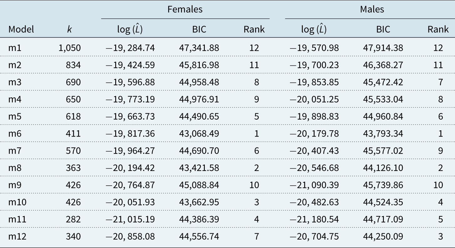
Table 7. BIC and log likelihood values for model m8 without cohort effect, with individual cohort effects and with common cohort effect. All models are fitted to IMD deciles for ages 40–89. The degrees of freedom are denoted by k.


Figure 15. Parameter estimates for model m8c with common cohort effects fitted to the female population.
7.1 Goodness of fit
To obtain further insights into the importance of cohort effects for model m8, we fit the model without a cohort effect, with individual effects and with common cohort effect to our data and compare the BICs. In Table 7, we report the obtained BIC values for males and females. For easy comparison, we also include the BIC values for the best fitting model m6.
We find in Table 7 that models with a common cohort effect are better suited to our data than models with no cohort effects or individual cohort effects. However, when we compare model m8 with a common cohort effect to our best fitting model m6, we notice that the results are not so clear. While model m8 with a common
 $\gamma$
outperforms model m6 for the male population, we find that the opposite is true for the female population. This suggests that the inclusion of non-parametric age effects in our model is more important for the female population than it is for the male population.
$\gamma$
outperforms model m6 for the male population, we find that the opposite is true for the female population. This suggests that the inclusion of non-parametric age effects in our model is more important for the female population than it is for the male population.
The quality of fit can be investigated further with the graphical diagnostics already applied in section 6. Heatmaps of standardised residuals are shown in Figure 16.

Figure 16. Heatmaps for standardised residuals from m8c (fitted to female population) with group-specific cohort effects
 $\gamma_{ci}$
for group 1 (left), group 5 (middle) and group 10 (right). Black cell: positive figures; Grey cell: negative figures.
$\gamma_{ci}$
for group 1 (left), group 5 (middle) and group 10 (right). Black cell: positive figures; Grey cell: negative figures.

Figure 17. Distribution of standardised residuals by m8c (fitted to female population) over age (left), year (middle) and cohort (right) for group 1 (top) and 10 (bottom) with
 $\gamma_{ci}$
applied. Colours in age and year plot represent different years/ages.
$\gamma_{ci}$
applied. Colours in age and year plot represent different years/ages.
Comparing the heatmaps in Figure 16 with those in Figure 10 we find that the inclusion of group-specific cohort effects removed the remaining structure observed in the residuals of model m8. This conclusion is confirmed further by comparing the standardised residuals for m8c plotted in Figure 17 with those shown in Figure 11.
Turning to the model with common cohort effect
 $\gamma_c$
, we again plot the heatmaps of the obtained residuals (see Figure 18). In this figure, we clearly observe that there is some (quadratic) structure along the age dimension present in the residuals for groups 1 and 10 that the common cohort effect is unable to capture. This is again an indication that model m6 with the non-parametric age effects is a better choice then model m8 with cohort effects. Plotting the residuals by age, year and cohort in Figure 19 clearly shows that there is some structure left in the residuals confirming this conclusion.
$\gamma_c$
, we again plot the heatmaps of the obtained residuals (see Figure 18). In this figure, we clearly observe that there is some (quadratic) structure along the age dimension present in the residuals for groups 1 and 10 that the common cohort effect is unable to capture. This is again an indication that model m6 with the non-parametric age effects is a better choice then model m8 with cohort effects. Plotting the residuals by age, year and cohort in Figure 19 clearly shows that there is some structure left in the residuals confirming this conclusion.

Figure 18. Heatmaps of standardised residuals fitted from m8c with common
 $\gamma_{c}$
(fitted to female population) in group 1 (left), 5 (middle) and 10 (right). Black cell: positive figures; Grey cell: negative figures.
$\gamma_{c}$
(fitted to female population) in group 1 (left), 5 (middle) and 10 (right). Black cell: positive figures; Grey cell: negative figures.

Figure 19. Distribution of standardised residuals by m8c with common cohort effect (fitted to female population) over age (left), year (middle) and cohort (right) for group 1 (top) and group 10 (bottom) with common
 $\gamma_{c}$
applied. Colours in age and year plot represent different years/ages.
$\gamma_{c}$
applied. Colours in age and year plot represent different years/ages.
Summarising the results in this section for the female population, we conclude that non-parametric age effects are a better choice than cohort effects for ensuring a good fit. However, for the male population, we have seen in Table 7 that model m8c with a common
 $\gamma$
has a lower BIC value than model m6. To compare the two models further (when fitted to the male population), we plot the heat maps for the residuals of models m6 and m8c in Figure 20.
$\gamma$
has a lower BIC value than model m6. To compare the two models further (when fitted to the male population), we plot the heat maps for the residuals of models m6 and m8c in Figure 20.

Figure 20. Heatmaps for standardised residuals from model m6 (top row) and model m8c (bottom row). Both models are fitted to the male population over the underlying data range for groups 1 (left), 5 (middle) and 10 (right). Black cell indicates positive residuals
 $Z_{xti}$
, and grey cell indicates negative values.
$Z_{xti}$
, and grey cell indicates negative values.
Comparing Figures 18 and 20, we notice that the residuals of model m8c (fitted to the male population, Figure 20) still show some structure in the age dimension for group 1. However, this structure is less obvious than what we observed for the female population (Figure 18), and it has disappeared completely for males in groups 5 and 10. Comparing the model m8c residuals to the residuals from model m6, we now find rather similar pictures for the two models. Those observations are in line with the better BIC value of m8c compared to m6 as model m8c is able to capture most of the structure in the male mortality data with much fewer parameters than model m6.
8. Conclusions
In this paper, we compared the goodness of fit of several multi-population mortality models to data for 10 similarly sized socio-economic groups. Our analysis suggests that models which allow for group-specific time trends outperform models with a common first-order period effect, in particular the Li and Lee model, suggesting that mortality improvements in the 10 IMD deciles are different. This reflects the very different improvement rates observed since the year 2000. For many applications, mortality projections will be required and choosing a model with individual period effects as suggested here will create the new challenge of finding a parsimonious multivariate time series model for the period effects in the 10 groups that produces meaningful projected rates.
Our other important conclusion from this empirical study is that models with common non-parametric age effects
 $\beta$
, like model m6, seem to provide a better fit than models with log death rates that increase linearly in age. Although the inclusion of a cohort effect can be beneficial (e.g. males m8c versus m6), its inclusion tends to be less significant if the model incorporates non-parametric age effects: that is, in models such as m8c the cohort effect is perhaps capturing what should really be modelled as age–period effects. Lastly, we found that individual age effects do not improve the fit of a model.
$\beta$
, like model m6, seem to provide a better fit than models with log death rates that increase linearly in age. Although the inclusion of a cohort effect can be beneficial (e.g. males m8c versus m6), its inclusion tends to be less significant if the model incorporates non-parametric age effects: that is, in models such as m8c the cohort effect is perhaps capturing what should really be modelled as age–period effects. Lastly, we found that individual age effects do not improve the fit of a model.
In summary, we conclude that the effect of age on mortality is similar in all socio-economic groups, while period effects are different.
It is also useful to remark that the preferred CAE model, m6, also satisfies the principle of coherence (Hyndman et al. Reference Hyndman, Booth and Yasmeen2013). Other models do not satisfy this principle, and so it is reassuring that the model that (mostly) has the lowest BIC value is coherent.
Our analysis is a first step towards projecting death rates in the 10 IMD deciles in England, but the empirical evidence found in our study suggests that mortality models for a country can be refined significantly by considering mortality patterns in different socio-economic groups.
Let us finish with a word of caution, the results presented in this paper are based on the data for England. Therefore, the results might be very different when other populations are considered, or even for data from the same population but for different ages and/or years. For instance, in Wen et al. (2020), we studied the multi-population models in Table 2 fitted to data for members of the CPP and the QPP, and we found a different ranking of models. However, it turned out that our preferred model, m6, for the IMD deciles is also our preferred model for the Canadian data, although it does not have the best BIC value for those data.
Mortality data by socio-economic groups are currently only available for relatively short periods; in this paper, we consider only 17 years of data. The age range is much wider, 50 years. This could be a reason for models with group-specific period effects to outperform models with common period effects as, in the long run, a common period effect could explain joint movements in all groups, which is hidden behind group-specific developments in short observation periods. While we have only considered this aspect very briefly, see Table 4 where the age range is restricted, we would suggest that this issue is investigated further, in particular, for applications that require the modelling of a narrow age range only, or where a longer history of mortality data is available.
Acknowledgements
The authors acknowledge financial support from the Actuarial Research Centre of the Institute and Faculty of Actuaries through the research programme on ‘Modelling, Measurement and Management of Longevity and Morbidity Risk’.
Appendix A Identifiability Constraints
Like many mortality models, most of the models in Table 2 require identifiability constraints to obtain unique parameter estimates. The only model not requiring any constraints in this study is model m12. For all other models, the constraints are listed in Table A.1.
Table A.1. List of constraints used in this study.

Appendix B Model Selection Criteria Using the IMD 2004 Ranking
Table B.1 shows the BIC values and the relative ranks of our 12 models fitted to mortality data for IMD deciles based on the LSOA rankings in 2004 rather than 2015. As mentioned in section 4.1, the order of models is similar in Tables 3 and B.1, in particular, model m6 outperforms all other models.
Table B.1. BIC and log likelihood values for all models fitted to IMD 2004 deciles for ages 40–89 and years 2001–2017. The degrees of freedom are denoted by k.


