


1 Introduction
Underfunding of defined benefit pension schemes is a significant risk to members of these schemes. For example, Milliman (2012) reports that the largest 100 defined benefit pension schemes of publically listed companies in the U.S. had an average funding level of less than 80% in 2011 whilst the Pension Protection Fund (PPF) and Pensions Regulator (2012) report a funding level of 83% at 31 March 2012 compared to the capped and hence, smaller liability that the PPF covers in the U.K. Scheme default insurance (known hereafter as “default insurance”), such as the PPF and the Pension Benefit Guaranty Corporation (PBGC) in the U.S., is designed to provide some protection to members of schemes which are unable to meet their promised obligationsFootnote 1.
However, the sliding levy scales based on funding levels and, for the PPF, the perceived risk of the employer-sponsor becoming insolvent, may affect investment and contribution decisions made in respect of the scheme in order to reduce the amount of levy paid. In addition, the PPF has recently introduced an allowance for investment risk into levy calculations. Hence, default insurance also has a separate indirect effect on the financial outcomes of the scheme due to the effect of the insurance on these investment and contribution decisions.
In addition to a desire to reduce levy payments, an attempt to game the default insurer may also affect investment and contribution decisions. This occurs when an employer-sponsor is happy to accept a lower level of funding knowing that the default insurer acts as a back-up where the scheme is unable to be continued. This game is most explicitly successful if the default insurer takes on the scheme liabilities whilst allowing the employer-sponsor to continue doing businessFootnote 2, however for an ongoing scheme the ability to participate in this game may be constrained by funding rules present in the country of operation. For example, in the U.K. trustees are required to have a statement of funding principles that outlines the funding approach to ensure assets are sufficient to meet the benefits accrued under the scheme. The requirements in the U.S. are more rigid, with prescribed assumptions and minimum contribution amounts depending on the financial position of the scheme. In any case, the advent of accounting standards (the international standard IAS 19, and associated country-based standards) which require the inclusion of pension scheme deficits on employer-sponsor balance sheets may somewhat reduce the attractiveness of this game.
In this paper a comprehensive stochastic asset and liability model is developed to investigate the effect that a default insurance system (based on the PPF) has on investment and contribution decisions in respect of a model scheme, and the resultant indirect effect on the financial stability of the scheme. The model allows separate investigation of the effects of a desire to reduce levy payments and/or to game the default insurer. The employer-sponsor and trustee are assumed to make these decisions in conjunctionFootnote 3; three competing employer-sponsor objectives are allowed for – the desire to reduce average contributions, the desire to reduce unexpected excess contributions and the desire to reduce funding deficits. The focus of the paper is therefore on the effect of default insurance systems on defined benefit schemes and not on the financial and moral viability of the default insurance systems themselves. The employer-sponsor objectives in relation to the scheme are treated separately from the other objectives of the business.
Whilst there is significant previous literature on the use of stochastic models for pension decision makingFootnote 4, there are few examples in the modelling literature on the effect of default insurance on these decisions. The literature in this field tends to be more theoretical in nature. Early PBGC-based studies focused on the incentives of the employer-sponsor to reduce funding levels and increase investment risk due to the put option offered by the PBGC protection (see for example Sharpe (Reference Sharpe1976), Treynor (Reference Treynor1977) and Niehaus (Reference Niehaus1990). A similar argument is made by Sutcliffe, Reference Sutcliffe2004). These incentives were exacerbated by the flat premium structure that was unrelated to the risks of the schemeFootnote 5 and hence did not penalise employers in terms of higher premiums for lower funding levels. Crossley & Jametti (Reference Crossley and Jametti2011) ran an empirical analysis on Canadian data and found that schemes backed by default insurance (i.e. those in Ontario) allocate around 5% extra of their assets to equities than schemes not backed by default insuranceFootnote 6.
One previous study that has considered the effect of the gaming element of default insurance is McCarthy & Miles (Reference McCarthy and Miles2007), who use a mathematical dynamic programming model to investigate the optimal equity allocation for a number of scenarios including the introduction of default insurance. They achieve this by adjusting the funding level to account for any deficit covered by insurance. The investment decision is set using a utility function approach on adjusted funding level. They find that default insurance increases the optimal allocation to equities, especially when funding levels are low. However, they do not make any allowance for contribution desires nor the cost of default insurance.
This paper takes a different modelling approach to that of McCarthy & Miles (Reference McCarthy and Miles2007). Firstly a simulation rather than a mathematical model is used. Secondly contribution decisions and desires are allowed for in the model in addition to investment decisions and funding level desires. These desires are also affected by the cost of default insurance in addition to a gaming motive. This combination of analysis is unique in the literature and provides the most comprehensive insight into the effect of default insurance on decisions made in respect of defined benefit pension schemes.
Section 2 of this paper outlines the methodology used in the analysis, whilst Section 3 provides the results. Conclusions are presented in Section 4.
2 Methodology
2.1 Simulation model
Assets and liabilities of a model scheme are projected over discrete annual periods for 30 years over 1,000 simulations using stochastic economic and demographic models. The 30 year period is chosen to represent the long-term nature over which pension decisions are typically made. During the projection period no explicit allowance is made for the potential for schemes to default, in order to ensure the optimisation process outlined in Section 2.3 is over a consistent time period for all simulations.
The economic model is based on the Wilkie (Reference Wilkie1995) structureFootnote 7, parameterised using Australian dataFootnote 8 over the period 30 June 1983 to 30 June 2009. Table 1 presents some basic statistics from the economic model across the 1,000 simulations.
Table 1 Basic statistics from the economic model

*Note that a promotional salary scale is also used to provide age-based increases.
Underlying withdrawal and mortality rates are also based on Australian experience, with mortality improvement also being allowed for. Uniform random numbers are compared to underlying withdrawal and mortality rates each year in simulating movements between membership status of individual members, as per the approach of Chang (Reference Chang1999).
The projection of assets and liabilities of the model scheme is similar in approach to that taken by the Stochastic Valuation Working Party of the U.K. Pensions Board (see Haberman et al., Reference Haberman, Day, Fogarty, Khorasanee, McWhirter, Nash, Ngwira, Wright and Yakoubov2003), with the exception that in this paper the normal contribution rate is fixed on a projected unit credit basis and the deficit spread period is treated as a free variable, whilst in Haberman et al. (Reference Haberman, Day, Fogarty, Khorasanee, McWhirter, Nash, Ngwira, Wright and Yakoubov2003) the normal contribution rate is treated as a free variable with a fixed deficit/surplus spread periodFootnote 9.
Further information about the simulation model (including the economic and demographic sub-models) can be found in Section 3 and Appendix B & C of Butt (Reference Butt2011a).
2.2 The model scheme
The model scheme has 5,000 active members, 1,680 deferred members and 1,920 pensioner members at the commencement of projections and is closed to new entrantsFootnote 10. It has initial assets exactly equal to the value of the funding liabilities. Benefits are generally paid in the form of a price-inflation indexed pension (deferred until age 65), except when a member leaves with less than 7 years of service in which case a lump sum is paid.
The liabilities targeted for funding purposes are discounted on a risk-freeFootnote 11 basis using best estimate assumptions. Hence the discount rate is determined with reference to long-term government bond yields and inflation-linked bond yields and demographic assumptions are the expected rates obtained from the relevant stochastic demographic model. Normal contributions are calculated annually as a percentage of salaries on a projected unit credit basis using the liability assumptionsFootnote 12, with no delay between the effective date of contribution calculations and their application.
In most cases tax on contributions and investment earnings is assumed to be 15%, as per the Australian superannuation system. No tax is applied to investment earnings backing pensions in paymentFootnote 13. The liability discount rate for pre-pensioner liabilities is also reduced by 15%.
Surplus levels are not capped in any way, although after the 30 year projection period surplus assets are distributed as additional benefits to members. Should a deficit occur after 30 years, it is immediately removed by the employer-sponsor making the net of tax contribution required to fund the deficit. The result of this assumption is that the employer-sponsor is assumed to be exposed to all underfunding risk but not benefit from any overfunding other than a reduction in default insurance levy payments and a reduction in normal contributions for future benefit accruals.
Further information about the model scheme can be found in Appendix A of Butt (Reference Butt2011a).
2.3 Optimisation process
2.3.1 Decision metrics
The desires of employers in sponsoring defined benefit schemesFootnote 14 can be summarised as making low and predictable contributions, with the scheme having a minimal balance sheet effect. However, these desires are generally not internally consistent; for example a desire for low contributions is obviously at odds with a desire for minimal balance sheet effect. Given these inconsistent desires, they must be balanced against each other in some way. Individual components similar to Haberman et al. (Reference Haberman, Day, Fogarty, Khorasanee, McWhirter, Nash, Ngwira, Wright and Yakoubov2003)Footnote 15 are weighted in a fashion simplified from Taylor (Reference Taylor2002)Footnote 16, giving the following objective function V:
 $$V\, = \, \bar{c}\, + \, \alpha \, \times \, {{\bar{c}}_{exc}}\, + \, \beta \, \times \, \overline{{Dfct}} $$
In the above equation,  $$$\bar{c}$$$
is the average contribution rate as a percentage of salaries over 30 years and
$$$\bar{c}$$$
is the average contribution rate as a percentage of salaries over 30 years and  $$${{\bar{c}}_{exc}}$$$
is the average contribution rate in excess of normal contributions over 30 years (including any contribution required to meet deficits after 30 years). Hence
$$${{\bar{c}}_{exc}}$$$
is the average contribution rate in excess of normal contributions over 30 years (including any contribution required to meet deficits after 30 years). Hence  $$${{\bar{c}}_{exc}}$$$
recognises the fact that employer-sponsors place additional weight on reducing unexpected contributions in addition to reducing normal contributions.
$$${{\bar{c}}_{exc}}$$$
recognises the fact that employer-sponsors place additional weight on reducing unexpected contributions in addition to reducing normal contributions.  $$$\overline{{Dfct}} $$$
is the mean level of deficit of assets to funding liabilities (treating surpluses as zero deficits) over 30 years, divided by the initial asset level for scaling. Since the employer-sponsor of the model scheme does not benefit from surplus apart from reduced contributions (see Section 2.2), it is appropriate to not allow for surplus in the objective function. The value V is calculated for each simulation of the model scheme, with an optimal strategy being one that minimises the average (or expected) value of V across 1,000 simulations of the model scheme. See Butt (Reference Butt2011a) for further details of the calculation of the component parts of the objective function.
$$$\overline{{Dfct}} $$$
is the mean level of deficit of assets to funding liabilities (treating surpluses as zero deficits) over 30 years, divided by the initial asset level for scaling. Since the employer-sponsor of the model scheme does not benefit from surplus apart from reduced contributions (see Section 2.2), it is appropriate to not allow for surplus in the objective function. The value V is calculated for each simulation of the model scheme, with an optimal strategy being one that minimises the average (or expected) value of V across 1,000 simulations of the model scheme. See Butt (Reference Butt2011a) for further details of the calculation of the component parts of the objective function.
It now remains to select parameter values α and β. Contributions in excess of expectations are assumed to have double the effect on the objective function compared to contributions up to expectations; choosing α = 1 ensures they are “double counted” in both  $$$\bar{c}$$$
and
$$$\bar{c}$$$
and  $$${{\bar{c}}_{exc}}$$$
. The value of β is set on a somewhat arbitrary basis to be equal to 8, although this ensures the total contribution effects
$$${{\bar{c}}_{exc}}$$$
. The value of β is set on a somewhat arbitrary basis to be equal to 8, although this ensures the total contribution effects  $$$\bar{c}$$$
and
$$$\bar{c}$$$
and  $$${{\bar{c}}_{exc}}$$$
make up a greater proportion of the objective function than deficitsFootnote 17.
$$${{\bar{c}}_{exc}}$$$
make up a greater proportion of the objective function than deficitsFootnote 17.
2.3.2 Optimisation tools
It is assumed that employer-sponsors have two tools available to them in meeting the desires described in Section 2.3.1. The first is the choice of investment strategy and the second is the speed at which scheme deficits are removed by additional contributions. A single decision is made for both of these choices at the commencement of projections and is not varied over the 30 year projection period.
The investment strategy is allowed to vary between equities and interest-based asset classes. Equities are split  $$$58 {1 \over 3}}$$$
% to domestic and
$$$58 {1 \over 3}}$$$
% to domestic and  $$$41\tfrac{2}{3} $$$
% to international, which is consistent with the typical split of Australian schemes. Interest-based assets are invested to cash flow match the liabilities as closely as possible. The methodology for calculating returns on cash flow matched assets can be found in the Appendix of Butt (Reference Butt2011b). The assets available for cash flow matched investment are invested in proportion with the liabilities to be cash flow matched; in other words each expected cash flow is matched to the same percentage depending on the interest-based assets availableFootnote 18. The split between equities and interest-based asset classes is allowed to vary from 0%–100% in the results. Asset allocations are rebalanced at the end of each year.
$$$41\tfrac{2}{3} $$$
% to international, which is consistent with the typical split of Australian schemes. Interest-based assets are invested to cash flow match the liabilities as closely as possible. The methodology for calculating returns on cash flow matched assets can be found in the Appendix of Butt (Reference Butt2011b). The assets available for cash flow matched investment are invested in proportion with the liabilities to be cash flow matched; in other words each expected cash flow is matched to the same percentage depending on the interest-based assets availableFootnote 18. The split between equities and interest-based asset classes is allowed to vary from 0%–100% in the results. Asset allocations are rebalanced at the end of each year.
Any deficit is spread (using the approach described by Owadally & Haberman, Reference Owadally and Haberman1999) using a range of spread periods from 1 – 20 years in the results. A shorter spread period results in a larger adjustment to normal contributions to remove the deficit faster. A fixed spread period of 5 years is used for surplus to reflect the specific interest in investigating the frequency and severity of deficit. The spread adjustment contribution is calculated as a fixed dollar amount, rather than a percentage of salaries, due to the reducing salaries in a closed scheme.
Optimisation of the asset allocation and deficit spread period is undertaken using a gradient descent approach (see Chapter 7.2 of Gosavi, Reference Gosavi2010).
2.3.3 Gaming the default insurer
As discussed in the introduction, an employer-sponsor may game the default insurer by accepting a lower level of funding knowing that the default insurer acts as a back-up where the scheme is unable to be continued. This can be investigated by revising the calculation of  $$$\overline{{Dfct}} $$$
in the objective function in Section 2.3.1. Two scenarios are tested. Firstly, in the small gaming scenario (SG),
$$$\overline{{Dfct}} $$$
in the objective function in Section 2.3.1. Two scenarios are tested. Firstly, in the small gaming scenario (SG),  $$$\overline{{Dfct}} $$$
is revised to only allow for deficits up to the value of the difference between the funding liability and the default liability (i.e. the actual “loss” by members due to default as the remaining deficit is covered by the default insurer). Secondly, in the large gaming scenario (LG),
$$$\overline{{Dfct}} $$$
is revised to only allow for deficits up to the value of the difference between the funding liability and the default liability (i.e. the actual “loss” by members due to default as the remaining deficit is covered by the default insurer). Secondly, in the large gaming scenario (LG),  $$$\overline{{Dfct}} $$$
is set to zero, reflecting no desire by the employer-sponsor to remove deficits (i.e. this is equivalent to setting β to zero). Note that under both scenarios contribution decisions are still made to target full funding, but the desire driving this decision has changed (i.e. only the calculation of one component of the objective function has changed, with the remainder of the model remaining consistent). Of course this may result in decisions that are unacceptably risky to Regulators, although this is not allowed for explicitly in the modelling.
$$$\overline{{Dfct}} $$$
is set to zero, reflecting no desire by the employer-sponsor to remove deficits (i.e. this is equivalent to setting β to zero). Note that under both scenarios contribution decisions are still made to target full funding, but the desire driving this decision has changed (i.e. only the calculation of one component of the objective function has changed, with the remainder of the model remaining consistent). Of course this may result in decisions that are unacceptably risky to Regulators, although this is not allowed for explicitly in the modelling.
2.4 Default insurance levy frameworks considered
2.4.1 Default insurance old (IO)
The old PPF model which applied until 31 March 2012 is used as a starting point. Note that only the risk-based portion of the levy is included as the scheme-based portion is similar to other expenses of the scheme which have been ignored. The risk-based levy, Lvy(t), paid during year t, based on liabilities,  $$$L(t\:{\rm{\, -\, }}\:{\rm{1}})$$$
, and Scheme assets,
$$$L(t\:{\rm{\, -\, }}\:{\rm{1}})$$$
, and Scheme assets,  $$$N(t\,{\rm{ - }}\,{\rm{1}})$$$
, at time t – 1 is:
$$$N(t\,{\rm{ - }}\,{\rm{1}})$$$
, at time t – 1 is:
 $$ Lvy(t)\, = \, \min \left[ {{\rm{0}}{\rm{.0075}}\, \times \, L(t\, {\rm{ - }}\, {\rm{1}}),U\, \times \, P\, \times \, {\rm{0}}{\rm{.8}}\, \times \, {\rm{2}}{\rm{.07}}} \right] $$
The liability L is the liability covered by the default insurer, and is based on a simplified version of the requirements of Section 179 of the Pensions Act 2004. It is identical to the funding liability outlined in Section 2.2, with the exception that all active members are assumed to withdraw at the valuation date and the PPF benefits are the minimum of 90% of the actual entitlement and a cap to be appliedFootnote 19 (see Appendix A for further details). Hence the default liability for levy calculations is always smaller than the liability for funding calculations. Scheme assets N are at market value, P is the employer-specific insolvency probability and U is the underfunding of the scheme and is calculated as:
 $$\openup 2ptU\, = \left\{ {\matrix{ {{\rm{1}}{\rm{.36}}\, \times \, L(t\, {\rm{\, -\, }}\, {\rm{1}})\, {\rm{ - }}\, N(t\, {\rm{ - }}\, {\rm{1}})} & {{\rm{if}}} & {N(t\, {\rm{ - }}\, {\rm{1}})\, \leq \, {\rm{1}}{\rm{.35}}\, \times \, L(t\, {\rm{ - }}\, {\rm{1}})} \hfill \cr {{\rm{0}}{\rm{.0100}}\, \times \, L(t\, {\rm{ - }}\, {\rm{1}})} & {{\rm{if}}} & {{\rm{1}}{\rm{.35}}\, \times \, L(t\, {\rm{ - }}\, {\rm{1}})\, \leq \, N(t\, - \, {\rm{1}})\, \lt \, {\rm{1}}{\rm{.40}}\, \times \, L(t\, {\rm{ - }}\, {\rm{1}})} \hfill \cr {{\rm{0}}{\rm{.0075}}\, \times \, L(t\, {\rm{ - }}\, {\rm{1}})} & {{\rm{if}}} & {{\rm{1}}{\rm{.40}}\, \times \, L(t\, {\rm{ - }}\, {\rm{1}})\, \leq \, N(t\, - \, {\rm{1}})\, \lt \, {\rm{1}}{\rm{.45}}\, \times \, L(t\, {\rm{ - }}\, {\rm{1}})} \hfill \cr {{\rm{0}}{\rm{.0050}}\, \times \, L(t\, {\rm{ - }}\, {\rm{1}})} & {{\rm{if}}} & {{\rm{1}}{\rm{.45}}\, \times \, L(t\, {\rm{ - }}\, {\rm{1}})\, \leq \, N(t\, {\rm{ - }}\, {\rm{1}})\, \lt \, {\rm{1}}{\rm{.50}}\, \times \, L(t\, {\rm{ - }}\, {\rm{1}})} \hfill \cr {{\rm{0}}{\rm{.0025}}\, \times \, L(t\, {\rm{ - }}\, {\rm{1}})} & {{\rm{if}}} & {{\rm{1}}{\rm{.50}}\, \times \, L(t\, {\rm{ - }}\, {\rm{1}})\, \leq \, N(t\, {\rm{ - }}\, {\rm{1}})\, \lt \, {\rm{1}}{\rm{.55}}\, \times \, L(t\, {\rm{ - }}\, {\rm{1}})} \hfill \cr {\rm{0}} & {{\rm{if}}} & {{\rm{1}}{\rm{.55}}\, \times \, L(t\, {\rm{ - }}\, {\rm{1}})\, \leq \, N(t\, {\rm{ - }}\, {\rm{1}})} \hfill \\\end\right$$
These formulae are consistent with the PPF levy for the period 1 April 2011 – 31 March 2012 (Pension Protection Fund, 2010a), with 0.8 being a parameter representing the percentage of the PPF levy to be collected based on scheme funding levels (the risk-based portion) and 2.07 being a parameter that ensures the PPF collects its targeted aggregate levy amount in 2011/12. This levy formula is assumed to apply across the whole simulation period. Since default events are not included in the modelling (see Section 2.1), for simplicity, the probability of insolvency P upon which the risk-based levy is based is assumed to be fixed across the 30 year projection period, with a range of P values tested corresponding to the old P values equivalent to the mid-points of the new levy bands to be used by the PPF in a new framework (see Section 2.4.2). This essentially means the P values tested reflect differing levels of levy payable rather than any direct impact of default.
Even though a Section 179 valuation is only required to be performed on a triennial basis, it is assumed that the levy calculation is based on the annually calculated default liability. The levy amount is assumed to be paid by the employer-sponsor as excess contributions, except where surplus is large enough that no contributions are required and the levy can be paid from surplus.
2.4.2 Default insurance new (IN)
Details of the new PPF levy framework for the period 1 April 2012 – 31 March 2013 can be found in a Consultation Document (Pension Protection Fund, 2011). This document describes adjustments to the levy framework introduced in Section 2.4.1 to follow the requirements of the new framework. The most significant change to the risk-based portion of the levy is that the underfunding risk U allows for smoothing of assets and liabilities over a 5 year period and for riskiness of the scheme's investment strategy (through a separate stress test on liabilities and assets). A Transformation Appendix to the 2012/13 Levy Policy Statement describes how the smoothing and riskiness of the scheme's investment strategy is allowed for. The remainder of this subsection describes briefly how this process is performed in this paper, which is much simpler than the requirements of the PPF due to the fact that a single indexation approach is assumed for all liabilities in the model scheme, unlike the requirements in the U.K.
Firstly, smoothing is applied to liability and asset valuesFootnote 20. The smoothed liability value at time t−1,  $$${{L}^{sm}} (t\,{\rm{ - }}\,{\rm{1}})$$$
, is calculated the same way as
$$${{L}^{sm}} (t\,{\rm{ - }}\,{\rm{1}})$$$
, is calculated the same way as  $$$L(t\,{\rm{ - }}\,1)$$$
in Section 2.4.1 but using the average discount rate applying over the previous 5 years. The smoothed value of bond classes are calculated assuming yields are equal to the average yield over the previous 5 years. No smoothing adjustment is made to cash. The smoothed value of equity classes are calculated by adjusting equity values to reflect the average dividend yield over the previous 5 years. See Appendix B for further information on how these calculations are performed.
$$$L(t\,{\rm{ - }}\,1)$$$
in Section 2.4.1 but using the average discount rate applying over the previous 5 years. The smoothed value of bond classes are calculated assuming yields are equal to the average yield over the previous 5 years. No smoothing adjustment is made to cash. The smoothed value of equity classes are calculated by adjusting equity values to reflect the average dividend yield over the previous 5 years. See Appendix B for further information on how these calculations are performed.
Secondly, stress tests are applied to smoothed liability and asset values to give adjusted liability and asset values  $$${{L}^{adj}} (t\,{\rm{ - }}\,1)$$$
and
$$${{L}^{adj}} (t\,{\rm{ - }}\,1)$$$
and  $$${{N}^{adj}} (t\,{\rm{ - }}\,{\rm{1}})$$$
. The stress tests are designed to allow for a one standard deviation movementFootnote 21 in the funding level. Appendix B to this paper provides information on how these stress tests are performed.
$$${{N}^{adj}} (t\,{\rm{ - }}\,{\rm{1}})$$$
. The stress tests are designed to allow for a one standard deviation movementFootnote 21 in the funding level. Appendix B to this paper provides information on how these stress tests are performed.
Thirdly, the formula for the risk-based levy is updated to:
 $$Lvy(t)\, = \, \min \left[ {{\rm{0}}{\rm{.0075}}\, \times \, {{L}^{sm}} (t\, {\rm{ - }}\, {\rm{1}}),U\, \times \, P\, \times \, {\rm{0}}{\rm{.89}}} \right];$$
In this equation  $$$U\: = \:\max \left[ {{\rm{0}},{{L}^{adj}} (t\,{\rm{ - }}\,{\rm{1}})\,{\rm{ - }}\,{{N}^{adj}} (t\,{\rm{ - }}\,1)} \right]$$$
and 0.89 represents a scaling factor to achieve the required levy of aggregate levy payments for the PPF in 2012/13. This levy formula is assumed to apply across the whole simulation period. A range of P values are tested, corresponding to the ten levy bands to be implemented. These levy bands represent a choice of ten different probabilities of insolvency that will be allocated to schemes in the new framework (see Table 1 in the Insolvency Risk Appendix of 2012/13 Levy Policy Statement). The equivalency of the P values tested between IO and IN is presented in Table 2.
$$$U\: = \:\max \left[ {{\rm{0}},{{L}^{adj}} (t\,{\rm{ - }}\,{\rm{1}})\,{\rm{ - }}\,{{N}^{adj}} (t\,{\rm{ - }}\,1)} \right]$$$
and 0.89 represents a scaling factor to achieve the required levy of aggregate levy payments for the PPF in 2012/13. This levy formula is assumed to apply across the whole simulation period. A range of P values are tested, corresponding to the ten levy bands to be implemented. These levy bands represent a choice of ten different probabilities of insolvency that will be allocated to schemes in the new framework (see Table 1 in the Insolvency Risk Appendix of 2012/13 Levy Policy Statement). The equivalency of the P values tested between IO and IN is presented in Table 2.
Table 2 P value bands
3 Results
Initially, a contour plot of the average values of the objective function where no default insurance exists is presented in Figure 1 for various equity allocations and deficit spread periods. A triangle is placed at the optimal equity allocation and deficit spread period. Note that this plot is of the same form presented in Butt (Reference Butt2011a).
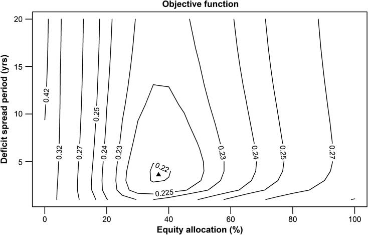
Figure 1 Objective function for no default insurance
The minimum value for the objective function of 0.2195 occurs at an equity allocation of 36.76% and a deficit spread period of 3.63 yearsFootnote 23. This is the optimal strategy to balance the contribution and funding level objectives set out in Section 2.3.1, giving an average contribution rate  $$$\bar{c}$$$
of 15.67%, an average excess contribution rate
$$$\bar{c}$$$
of 15.67%, an average excess contribution rate  $$${{\bar{c}}_{exc}}$$$
of 2.38% and a mean funding deficit
$$${{\bar{c}}_{exc}}$$$
of 2.38% and a mean funding deficit  $$$\overline{{Dfct}} $$$
of 0.4874%. Equity exposures smaller than 36.76% reduce excess contributions and funding deficits, but are more than offset by the higher payment of normal contributions due to the smaller probability of being in surplus. A shorter deficit spread period also reduces funding deficits, but at too much of a cost to excess contribution levels. Moving towards the top right corner of the plot by increasing equities and deficit spread period affects the objective function in a smaller way, although lower average contribution rates are not significant enough a compensation for larger excess contributions and funding deficits.
$$$\overline{{Dfct}} $$$
of 0.4874%. Equity exposures smaller than 36.76% reduce excess contributions and funding deficits, but are more than offset by the higher payment of normal contributions due to the smaller probability of being in surplus. A shorter deficit spread period also reduces funding deficits, but at too much of a cost to excess contribution levels. Moving towards the top right corner of the plot by increasing equities and deficit spread period affects the objective function in a smaller way, although lower average contribution rates are not significant enough a compensation for larger excess contributions and funding deficits.
The mean deficit of 0.4874% can be treated as a measure of the risk being faced by members of the scheme, as it reflects the size and likelihood of a deficit event that may result in a claim to the default insurer and subsequent lower level of benefit payment to members from the default insurer (see Section 2.4.1). A separate measure of the mean deficit to the capped default liability level (see Section 2.4.1) can be thought of as a measure of the risk being faced by the default insurer, as this is the amount that is required to be made up by the default insurer upon the default of the employer-sponsor of the scheme. Although the initial results do not include an allowance for default insurance levies, this mean capped deficit can still be calculated as 0.0321%.
Figures 2–5 show the impact of both old (IO) and new (IN) default insurance levy frameworks and the gaming scenarios SG and LG on the results described above. Figures 2 and 3 show the optimal equity allocations and deficit spread periods respectively. Figures 4 and 5 show the resultant mean deficits and mean capped deficits respectively.

Figure 2 Optimal equity allocations
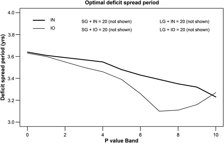
Figure 3 Optimal deficit spread periods

Figure 4 Mean deficits

Figure 5 Mean capped deficits
We first consider the effect of levy frameworks (IN and IO) without a gaming motive. In this case movements in the equity allocation and deficit spread period are designed to reduce levy payments, whilst not sacrificing other elements of the objective function. The old default insurance levy framework (IO) causes an increase in the optimal equity allocation, which can be seen in the upward sloping nature of the IO lines in Figure 2. The optimal equity allocation increases from 36.76% to 44.60% under IO from Band 0 to Band 10, a result broadly consistent with the empirical observations of Crossley & Jametti (Reference Crossley and Jametti2011). The deficit spread years for IO in Figure 3 initially decrease from 3.63 in Band 0 to 3.10 in Band 7, but then increase back to 3.27 years in Band 10.
Reducing levy payments, whilst not sacrificing other elements of the objective function, can be achieved in two ways for IO. Firstly, levy payment reduction can be achieved by reducing equity exposure and reducing deficit spread years, leading to a reduced probability of severe deficits. This explains the observed initial decrease in the deficit spread years for IN in Figure 3. The upturn in deficit spread years after Band 7 is due to the 0.75% liability cap on levy payments, which results in the levy not being reduced when deficits are reduced for schemes in a high P value BandFootnote 24. A second approach to levy payment reduction is to increase the equity exposure with the resultant aim of increasing the funding level. For IO, the second approach is more significant than the first in determining the optimal equity allocation, with the allocation increasing as the P value Band increases. A significant reason for this is that the risk-based levy does not cut out until the PPF funding level reaches 155% (see Section 2.4.1), encouraging an investment strategy that seeks a possibility of surplus. This is a particular concern as it means that schemes with a less stable employer-sponsor are exposed to greater risk of deficit, which can be seen in Figures 4 and 5. The mean deficit increases from 0.4874% to 0.5362% from Band 0 to Band 10 for IO in Figure 4 with an increase in mean capped deficit from 0.0321% to 0.0466% in Figure 5. Hence the indirect effect of the levy framework under IO is to put both members and the default insurer at greater risk.
What is most interesting about this result is that this incentive to increase investment risk as P value Band increases exists without any benefit of surplus or attempt to game the default insurer. Whilst the levy calculations of the PBGC do not incorporate probability of employer-sponsor insolvency, they do allow for funding position. Hence the above results infer that a PBGC-style framework also increases the optimal allocation to equities, but on a consistent level for all schemes regardless of the strength of the employer-sponsor.
Incorporating investment risk into the new default insurance levy framework (IN) leads to a third way in which levy payments can be reduced. Decreasing equity exposure reduces the effect of the stress testing on levy payments. This third approach to reducing levy payments weights the decision in favour of a decrease in the optimal equity allocation from 36.76% to 35.41% from Band 0 to Band 10 in Figure 2. There is hence a total reduction in optimal equity allocation between IO and IN of 9.19% for Band 10. This is consistent with the maximum change of optimal asset allocation of 8.5% noted by the Pension Protection Fund (2010b) in its analysis of the effect of including investment risk in levy calculations on scheme asset allocation. A continual decrease in deficit spread years is observed under IN from 3.63 years to 3.23 years in Figure 3, as the relatively low optimal equity allocations, and hence relatively small deficits, mean the levy cap is typically not applied under IN.
These results lead to an opposite indirect effect of default insurance under IN, with the mean deficit decreasing from 0.4874% to 0.4521% from Band 0 to Band 10 in Figure 4 and mean capped deficit decreasing from 0.0321% to 0.0229% in Figure 5. These are significant results in demonstrating a strong rationale for the change in levy framework introduced by the PPF.
Looking now at the effect of an employer-sponsor attempting to game the default insurer, there is a clear and significant impact on the optimal equity allocation in Figure 2. Where no levy is paid, an employer-sponsor who is not concerned about deficits below the default insurance liability level (SG) has an increase in optimal equity allocation from 36.76% to 55.19%, whilst an employer-sponsor who is not concerned about any deficit (LG) has an increase to 74.51%. These represent increases of 18.43% and 37.75% for SG and LG respectively. These significant increases in investment risk taken on are due to the reduced weighting to the risk of being in deficit under SG and LG, allowing the employer-sponsor to attempt to reduce contributions by taking on this investment risk. This is consistent with the theoretical results of previous papers such as Sutcliffe (Reference Sutcliffe2004) relating to the PBGC in the U.S., even though the objective function in this paper does not provide any benefit for surplus. However, the increase is much higher than that observed by Crossley & Jametti (Reference Crossley and Jametti2011), with equity allocations for schemes in Canada under the effect of default insurance being consistent with an attempt to reduce levy payments rather than trying to game the default insurer. The effect of IO compared to IN on optimal equity allocation is broadly similar irrespective of the gaming approach used by the employer sponsor, with the shapes of the IN and IO lines in Figure 2 being relatively consistent and a Band 10 difference between IN and IO optimal equity allocations of 15.21% for SG and 16.98% for LG compared to 9.19% for no gaming.
In Figure 3 the deficit spread years for SG and LG are not shown as they are at the maximum level allowed for in the study of 20 years for all IO and IN Bands. The inference here is that there is no need for employer-sponsors to reduce deficits through extra contributions. This is because expected investment returns rather than extra contributions can be used to reduce the deficit without any potential additional objective function losses from larger deficits resulting from possible poor investment performance, as deficits under the objective function are either capped (SG) or not allowed for (LG).
These significant changes to optimal equity allocation and deficit spread period flow through to significant differences in the deficits affecting members and the default insurer. Taking IN Band 10 as an example, the mean deficit increases from 0.4521% to 1.0079% under SG in Figure 4 and 1.2295% under LG in Figure 5. The mean capped deficit increases from 0.0183% to 0.3152% under SG in Figure 4 and 0.4660% under LG in Figure 5. These results indicate that employer-sponsors attempting to game the default insurer have a very significant negative impact on the risks faced by scheme members and the default insurer. This is independent of the structure of the levy amount and hence is also relevant for frameworks that base the levy on a fixed percentage of liabilities only.
4 Conclusions
This paper has considered the effect of two scheme default insurance levy frameworks and the effect of gaming the default insurer on the optimal equity allocation and deficit spread period of a model defined benefit pension scheme which is closed to new entrants. The objective in determining optimal equity allocation and deficit spread period considers a balance of reducing average contribution levels, average contribution levels in excess of normal contributions and the mean funding deficit of assets to liabilities (treating surpluses as zero deficits). The gaming of the default insurer is tested by adjusting the deficit objective.
It is found that the old default insurance levy framework used by the PPF, which bases levy payments on funding level and probability of employer-sponsor insolvency, leads to an increase in the optimal allocation to equities as the insolvency probability increases, due to the desire to move the scheme into surplus and thus reduce levy payments. The effect on deficit levels is offset by a reduction in optimal deficit spread years, although the 0.75% liability cap on levy payments ceases this reduction for schemes which are at significant risk. Overall, the effect of the old insurance levy framework on optimal decisions leads to an indirect increase in deficit levels experienced, affecting both members and the default insurer, which is largest for schemes which are most at risk. Frameworks that allow for funding level but not insolvency probability in levy calculations (such as the PBGC in the U.S.) also have this indirect effect on deficit levels, although it is consistent for all employers.
The new PPF framework reverses this feedback effect, due to its consideration of investment risk in the levy calculations. Hence, under this framework it is optimal for schemes to reduce their allocation to equities by close to 10% compared with the old framework, in order to reduce investment risk and thus levy payments. Deficit levels affecting members and the default insurer are up to 16% and 51% lower respectively under the new framework.
However, employer-sponsors who wish to game the default insurer have much larger optimal equity allocations and deficit spread periods, leading to deficits affecting members and the default insurer which are 123–172% and 1277–1935% larger respectively for schemes under the new framework which are most at risk of default, depending on the level of gaming undertaken by the employer-sponsor. These results hold for other levy frameworks as well, indicating the very presence of default insurance can have a significant impact on the decisions made by employer-sponsors. However, comparing empirical evidence of asset allocation to the results of this paper indicates the average employer is not gaming the default insurer.
The results of this study are dependent and limited by the range of assumptions made in Section 2. In particular, future research could consider the following extensions:
• The effect of alternative stochastic models;
• Allowing for dynamic decision makingFootnote 25 depending on such factors as funding level and non-pension objectives of the employer-sponsor, etc.;
• Testing the outcomes on schemes which are open to new entrants or closed to all future accrualsFootnote 26;
• The effect of alternative objective functionsFootnote 27; and
• Allowing insolvency probability to vary stochastically and for the employer-sponsor to explicitly target the avoidance of default as a key objective.
Default insurance provides clear benefits to members of defined benefit pension schemes; however the design of the levy framework can lead to indirect effects that negatively impact on members and the default insurer. This study has shown that the introduction of investment risk into levy calculations is a positive move in removing the negative indirect effects associated with frameworks that treat risk by considering funding level and employer-sponsor insolvency risk only. However, the risk of employer-sponsors using default insurance to reduce their attitude to meeting deficit levels is a significant risk for both members and default insurers and a risk that appears to be simply inherent to the design of default insurance.
Acknowledgements
This paper provides some updated results of the PhD thesis of the author. All acknowledgements relevant to the PhD thesis are also relevant to this paper. In addition, the assistance of Huan Zhang, a research assistant at ANU, was vital to the completion of this paper. The author also wishes to thank seminar participants at the Pension, Benefits and Social Security Colloquium (Edinburgh, 2011) of the International Actuarial Association and also two anonymous reviewers of this journal for their helpful comments. Any errors or omissions remain the responsibility of the author.
Appendix A – Benefit cap applied for default liabilities for levy calculations
Section 2.4.1 describes the calculation of default liabilities for levy calculations. One aspect of this calculation is a cap on the benefits to be paid from the scheme. The cap is based on a similar approach used by the PPF, adjusted for the currency of the model scheme. Sample cap figures at the commencement of projections are presented in Table 3 (these are indexed by the salary inflation from the economic model each year).
Table 3 Benefit cap at the commencement of projections
Appendix B – Calculation of asset and liability values for scenario IN
To calculate the smoothed bond values, the actual bond yields used in the calculation of bond returns for the year to time t – 1 are replaced with the average bond yields over the previous 5 years. For example, the average long-term interest rate over the previous 5 years to time t – 1,  $$$\overline{{il'(t\,{\rm{ - }}\,{\rm{1}})}} $$$
, is calculated as follows:
$$$\overline{{il'(t\,{\rm{ - }}\,{\rm{1}})}} $$$
, is calculated as follows:
 $$\overline{{il'(t\, {\rm{ - }}\, {\rm{1}})}} = \frac{{il'(t\, {\rm{ - }}\, {\rm{6}})\, + \, {\rm{2}}\, \times \, il'(t\, {\rm{ - }}\, {\rm{5}})\, + \, {\rm{2}}\, \times \, il'(t\, {\rm{ - }}\, {\rm{4}})\, + \, {\rm{2}}\, \times \, il'(t\, {\rm{ - }}\, {\rm{3}})\, + \, {\rm{2}}\, \times \, il'(t\, {\rm{ - }}\, {\rm{2}})\, + \, il'(t\, {\rm{ - }}\, {\rm{1}})}}{{{\rm{10}}}} \ ^ {28}$$
Here,  $$$il'(t)$$$
is the long-term interest rate at time t. This calculation is performed separately for long-term interest rates and inflation-linked bond yields, which feed into the calculation of the smoothed values for Australian bonds, international bonds and inflation-linked bonds. Similarly, Australian equity market values are smoothed by adjusting the dividend yield to be equal to the average dividend yield over the previous 5 years. A consistent adjustment is made to international equity market values as the dividend yield is only calculated for Australian equities in the economic model.
$$$il'(t)$$$
is the long-term interest rate at time t. This calculation is performed separately for long-term interest rates and inflation-linked bond yields, which feed into the calculation of the smoothed values for Australian bonds, international bonds and inflation-linked bonds. Similarly, Australian equity market values are smoothed by adjusting the dividend yield to be equal to the average dividend yield over the previous 5 years. A consistent adjustment is made to international equity market values as the dividend yield is only calculated for Australian equities in the economic model.
Stress testing is then applied to the smoothed liability and asset values in a way consistent with the indicative stress approach of the Transformation Appendix of Pension Protection Fund (2011)Footnote 29. An identical approach to the PPF is not taken for a number of reasons, most importantly that the PPF based its calculations on U.K. investment data whilst the model in this paper was parameterised using Australian data. The following approach is taken:
• The average and standard deviation of funding level of the 1,000 simulations at time 1 is obtained, using the Base scenario and a 50% equity allocation. This gives a funding level, at one standard deviation away from the average, of 94.0%.
• Price inflation, long-term interest rates, inflation-linked bond yields and returns on equities are identified as the most significant drivers of movement in funding level. Simulations of the first year are re-run, allowing the error terms of these drivers to vary in proportion to their standard error in the economic model. All other error terms are held at zeroFootnote 30. The error terms that achieve an average funding level of 94.0% are identified in this processFootnote 31.
• Based on the results on the previous point, the following stressesFootnote 32 are applied to smoothed liability and asset values. Bond values are calculated using the same process described for smoothing, but using stressed yields. Price inflation is incorporated into both liability calculations and inflation-linked bond values. Cash values are unadjusted.
Making these adjustments provides the final adjusted liability and asset values,  $$${{L}^{adj}} (t\,{\rm{ - }}\,{\rm{1}})$$$
and
$$${{L}^{adj}} (t\,{\rm{ - }}\,{\rm{1}})$$$
and  $$${{N}^{adj}} (t\,{\rm{ - }}\,{\rm{1}})$$$
, to be used in the levy calculations. Stress tested assets for cash flow matched interest-based investment are assumed to have the same value as the stress tested liabilities, as unhedged liability factors such as salary increases and mortality rates are not allowed for in the stress testing.
$$${{N}^{adj}} (t\,{\rm{ - }}\,{\rm{1}})$$$
, to be used in the levy calculations. Stress tested assets for cash flow matched interest-based investment are assumed to have the same value as the stress tested liabilities, as unhedged liability factors such as salary increases and mortality rates are not allowed for in the stress testing.


