

1. Introduction
Many marketers of consumer products have noticed that, as part of their marketing campaign, they can offer insurance cover for their products for sale, such as free car insurance for a new car or specific insurance for a new piece of home electronics. Often the insurance cover is not provided by the marketers themselves but through a partnership agreement with an insurance provider, which may see this as one of its distribution channels. As a consequence, consumers will have different insurance cover for many of their products, most probably from different insurance providers, and except from losing the possibility to get a bundling discount, on insurances from the same insurer, the consumers will experience few negative effects with having multiple insurance providers. However, from an insurance company's point of view, providing only a single or few insurance products to a customer is seldom desirable since such customers are more likely to cancel their existing business with the company in favour of a competitor, see Kamakura et al. (Reference Kamakura, Wedel, de Rosa and Mazzon2003) for a general discussion about cross-selling as a method for retaining customers and Brockett et al. (Reference Brockett, Golden, Guillén, Nielsen, Parner and Perez-Marin2008) for an overview on how much time is left to stop total customer defection. Hence, insurance companies would be interested in developing their sales methods for increasing the number of products for their existing customers.
Increasing the number of products of a company's existing customers is referred to as cross-selling. In most cases this means personal communication, often through call-centres, with the customers for which the expected demand for a certain product is high. In this paper it is argued that for some businesses, especially insurance business, there is an alternative to this sales driven cross-selling approach. Unlike conventional retail products, insurance products are associated with costs that are stochastic and determined at a stochastic time interval after a sale has been made. This stochasticity implies that, from an insurer's point of view, also the profitability for a certain customer is stochastic. However, the profitability might be predictable and hence reveal sets of customers which are preferable for the insurance company to extend the existing business with. This paper contributes with a method for such profitability predictions not found in either the marketing or the actuarial literature. In the data study in Section 4, it is shown that the proposed method produces sets of customers with up to 36% less claims than expected. While this is just one example for one particular data set it still suggests that the method would be useful in practice.
The marketing literature on cross-sale models focuses primarily on various ways to model the demand for a certain cross-sale product amongst a company's customers. Often different regression models are evaluated based on data for the sales response of past cross-sale attempts, where patterns of the customers with high demand is sought after. One of the first efforts to model a cross-sale opportunity formally is Kamakura et al. (Reference Kamakura, Ramaswami and Srivastava1991), where a latent trait model is presented for the probability that a consumer would use a particular product or service, based on their ownership of other products or services. Another study is made by Knott et al. (Reference Knott, Hayes and Neslin2002) where a comparison is made of four different models for the probability of a successful cross-sale. Kamakura et al. (Reference Kamakura, Wedel, de Rosa and Mazzon2003) discuss reasons why cross-selling is crucial for financial services (such as banks and insurance companies) and present a predictive model for whether or not customers satisfy their needs for financial services elsewhere. They argue that when a customer acquires more products or services from the same company, the switching cost of the customer increases and thereby minimises the risk of the customer leaving for a competitor. In Li et al. (Reference Li, Sun and Wilcox2005) a natural ordering in which to present different products to a customer is investigated. They model the development over time for customer demand of multiple products and apply latent trait analysis to position financial services at correct time points within the customer lifetime.
The cross-sale method presented in this paper uses developments in multivariate credibility theory, for calculating a customer i's expected profitability of the cross-sale insurance product k with available data from another insurance product k′. The actuarial research branch of credibility theory investigates how collective and individual information should be weighted to produce a fair insurance premium for each individual. The literature on the subject is rich, dating back to early papers by Mowbray (Reference Mowbray1914) and Whitney (Reference Whitney1918) which are the first studies of what later became known as credibility theory. Pioneering papers on credibility theory are Bühlmann (Reference Bühlmann1967) and Bühlmann & Straub (Reference Bühlmann and Straub1970) where in the latter paper the Bühlmann-Straub credibility estimator is derived. Credibility estimators and Bayesian statistics are investigated in e.g. Bailey (Reference Bailey1950), Jewell (Reference Jewell1974) and Gangopadhyay & Gau (Reference Gangopadhyay and Gau2007). This paper uses developments of multivariate credibility found in Englund et al. (Reference Englund, Guillén, Gustafsson, Nielsen and Nielsen2008) and Englund et al. (Reference Englund, Gustafsson, Nielsen and Thuring2009), both papers model frequency of insurance claims from correlated business lines. Multivariate credibility models are also found in Venter (Reference Venter1985), describing multivariate credibility models in a hierarchical framework, and Jewel (Reference Jewel1989), investigating multivariate predictions of first and second order moments in a credibility setting. More recent references are Frees (Reference Frees2003), who applies multivariate credibility models for predicting aggregate loss, and Bühlmann & Gisler (Reference Bühlmann and Gisler2005), which is one of the standard references in credibility theory.
The structure of the paper is as follows. In Section 2 the credibility model is described and the estimator is presented for the case of complete data for both products. In Section 3 the multivariate credibility estimator for cross-selling is presented for the case of unavailable information for the cross-sale product k. In Section 4 the cross-sale method is tested and analysed on a large data set from the personal lines of business of a Danish insurance company and concluding remarks are found in Section 5.
2. The credibility model and estimator
We use the model from Englund et al. (Reference Englund, Guillén, Gustafsson, Nielsen and Nielsen2008) and estimation following Englund et al. (Reference Englund, Gustafsson, Nielsen and Thuring2009). We consider insurance customers i = 1 ,…, I in time periods j = 1 ,…, Ji with insurance products k′ and k, for convenience we will use the index l ∈ k′, k and r ∈ k′, k for insurance products in general. The insurance customer i is characterised by his/her individual risk profile θil which is a realisation of the independent and identically distributed random variable Θil, with E[Θil] = θ 0l and Cov[Θil, Θir] = ![]() with l, r ∈ {k′, k}, θ 0l is often called the collective risk profile. The number of insurance claims Nijl is assumed to be a Poisson distributed random variable with conditional expectation E[Nijl | Θil] = λijlΘil and the pairs (Θ1l, N 1jl), (Θ2l, N 2jl) ,…, (ΘIl, NIjl) are independent. We have a priori expected number of claims
with l, r ∈ {k′, k}, θ 0l is often called the collective risk profile. The number of insurance claims Nijl is assumed to be a Poisson distributed random variable with conditional expectation E[Nijl | Θil] = λijlΘil and the pairs (Θ1l, N 1jl), (Θ2l, N 2jl) ,…, (ΘIl, NIjl) are independent. We have a priori expected number of claims ![]() of customer i in period j and product l ∈ k′, k, which depends on the exposure eijl, a regression function gl and of a set of explanatory tariff variables
of customer i in period j and product l ∈ k′, k, which depends on the exposure eijl, a regression function gl and of a set of explanatory tariff variables ![]() characterising the customer and the insured object. Note that gl is common for all customers i and time periods j and is estimated based on collateral data from the insurance company. We assume that eijl can take values between [0; 1], where eijl = 0 means that the l-th product is not active for customer i in time period j and correspondingly, eijl = 1 means that the product l of customer i is active during the entire time period j. We define
characterising the customer and the insured object. Note that gl is common for all customers i and time periods j and is estimated based on collateral data from the insurance company. We assume that eijl can take values between [0; 1], where eijl = 0 means that the l-th product is not active for customer i in time period j and correspondingly, eijl = 1 means that the product l of customer i is active during the entire time period j. We define ![]() , which is a measure of the deviation between the a priori expected number of claims λijl and the observed number of claims Nijl. Further we assume that the insurance premium Pijl is proportional to λijl and that the claim severities
, which is a measure of the deviation between the a priori expected number of claims λijl and the observed number of claims Nijl. Further we assume that the insurance premium Pijl is proportional to λijl and that the claim severities ![]() , v = 1,2,…,Nijl are independent and also independent of Nijl with
, v = 1,2,…,Nijl are independent and also independent of Nijl with ![]() . Analogous to the claim frequency,
. Analogous to the claim frequency, ![]() is a set of explanatory variables and hl a regression function. Note that E[Fijl | Θil] = Θil and, under the stated assumptions, the lower the individual risk profile θil is, the higher the profitability is. We assume a conditional covariance structure of Fijl as
is a set of explanatory variables and hl a regression function. Note that E[Fijl | Θil] = Θil and, under the stated assumptions, the lower the individual risk profile θil is, the higher the profitability is. We assume a conditional covariance structure of Fijl as ![]() and Cov[Fijk ′, Fijk | Θik ′, Θik] = 0, where
and Cov[Fijk ′, Fijk | Θik ′, Θik] = 0, where ![]() is the variance within an individual customer i, for l ∈ k′, k. With
is the variance within an individual customer i, for l ∈ k′, k. With ![]() and
and ![]() we get
we get ![]() and Cov[Fi ·k ′, Fi ·k | Θik ′, Θik] = 0. Since we consider the two-dimensional case with the specific insurance products k′ and k, under the stated model assumptions, the multivariate credibility estimator of θi = [θik ′, θik]′ is (see Englund et al., Reference Englund, Gustafsson, Nielsen and Thuring2009 and Bühlmann & Gisler Reference Bühlmann and Gisler2005, p. 181)
and Cov[Fi ·k ′, Fi ·k | Θik ′, Θik] = 0. Since we consider the two-dimensional case with the specific insurance products k′ and k, under the stated model assumptions, the multivariate credibility estimator of θi = [θik ′, θik]′ is (see Englund et al., Reference Englund, Gustafsson, Nielsen and Thuring2009 and Bühlmann & Gisler Reference Bühlmann and Gisler2005, p. 181)
with ![]() . The credibility weight αi = TΛi(TΛi + S)−1 where
. The credibility weight αi = TΛi(TΛi + S)−1 where ![]() ,
, ![]() and
and ![]() , see Englund et al. (Reference Englund, Gustafsson, Nielsen and Thuring2009). The parameters
, see Englund et al. (Reference Englund, Gustafsson, Nielsen and Thuring2009). The parameters ![]() and
and ![]() are equal to
are equal to ![]() and
and ![]() , respectively. We are considering a homogeneous credibility estimator and we therefore need an estimator for the collective risk profiles θ 0k ′ and θ 0k. An unbiased estimator is found in Bühlmann & Gisler (Reference Bühlmann and Gisler2005, p. 183) as
, respectively. We are considering a homogeneous credibility estimator and we therefore need an estimator for the collective risk profiles θ 0k ′ and θ 0k. An unbiased estimator is found in Bühlmann & Gisler (Reference Bühlmann and Gisler2005, p. 183) as ![]() . Performing the matrix multiplication in (1) gives the multivariate credibility estimator of θik, for the specific product k, based on Fi ·k ′ and Fi ·k as,
. Performing the matrix multiplication in (1) gives the multivariate credibility estimator of θik, for the specific product k, based on Fi ·k ′ and Fi ·k as,
For the estimation procedure of the parameter matrices S and T see e.g. Bühlmann & Gisler (Reference Bühlmann and Gisler2005) p. 185–186 or Englund et al. (Reference Englund, Gustafsson, Nielsen and Thuring2009).
3. Cross-selling with the credibility estimator
We are interested in cross-selling an insurance product k to a set Φ of customers already having another insurance product k′ from the insurance company. The hypothesis is that an estimator ![]() , of the risk profile θik, can be obtained, based only on the available data for Fi ·k ′ with respect to the existing product k′, and that a profitable cross-sale set Φ* would consist of customers with as low
, of the risk profile θik, can be obtained, based only on the available data for Fi ·k ′ with respect to the existing product k′, and that a profitable cross-sale set Φ* would consist of customers with as low ![]() as possible. Prior to cross-selling product k to the i-th customer, product k is inactive and no claims have been reported i.e. nijk = 0. Also the exposure eijk = 0, with respect to the cross-sale product k, which leads to αikk = 0 and
as possible. Prior to cross-selling product k to the i-th customer, product k is inactive and no claims have been reported i.e. nijk = 0. Also the exposure eijk = 0, with respect to the cross-sale product k, which leads to αikk = 0 and ![]() in (2). The credibility estimator of θik, based only on the available Fi ·k ′, becomes
in (2). The credibility estimator of θik, based only on the available Fi ·k ′, becomes
Note that, in order to be able to evaluate (3), estimates of θ 0k, ![]() ,
, ![]() ,
, ![]() and θ 0k ′ need to be obtained from a collateral data set consisting of customers with both products k and k′ active and whose characteristics are as close to the characteristics of the customers, for which an estimate of the risk profile θik is sought after.
and θ 0k ′ need to be obtained from a collateral data set consisting of customers with both products k and k′ active and whose characteristics are as close to the characteristics of the customers, for which an estimate of the risk profile θik is sought after.
Considering that ![]() , a customer i with Fi ·k ′ < 1 has reported fewer insurance claims than a priori expected (for the existing product k′) and has therefore been a more profitable customer than a customer i′ with Fi ′·k ′ > 1. Hence, from the insurance company's point of view, a customer i is preferred over a customer i′ if
, a customer i with Fi ·k ′ < 1 has reported fewer insurance claims than a priori expected (for the existing product k′) and has therefore been a more profitable customer than a customer i′ with Fi ′·k ′ > 1. Hence, from the insurance company's point of view, a customer i is preferred over a customer i′ if ![]() and the expected most profitable set Φ* of size φ* to cross-sale a product k to is the first φ* customers when ordered by increasing
and the expected most profitable set Φ* of size φ* to cross-sale a product k to is the first φ* customers when ordered by increasing ![]() as
as
There are two ways to select the cross-sale set Φ*. Either by setting φ* to a predefined number of customers and using (4) to define Φ* or by setting an upper limit θL for which all customers with ![]() are in Φ*. A similar remark is made in Knott et al. (Reference Knott, Hayes and Neslin2002) regarding the probability of a successful cross-sale. We define the expected average profitability for a cross-sale set Φ as
are in Φ*. A similar remark is made in Knott et al. (Reference Knott, Hayes and Neslin2002) regarding the probability of a successful cross-sale. We define the expected average profitability for a cross-sale set Φ as
We also define the corresponding observed value ![]() as
as
where the weighting with αikk is needed for an unbiased comparison between ![]() and
and ![]() .
.
4. Data study
We have a large data set available from the personal lines of business of a Danish insurance company consisting of number of claims nijl (assumed to be realisations of a Poisson distributed random variable Nijl~Po(λijlΘil)) and a priori expected number of claims λijl, for 3 different insurance products, l ∈ {1,2,3} where l = 1 represents motor insurance, l = 2 represents building insurance and l = 3 represents content insurance. There are 95668 unique customers in the data set who all have active products {1,2,3} during the Ji years of engagement with the company. The number Ji is individual, between 1 and 5, and each record is unique for customer i in time period j making the total number of records in the data set 306196. Figure 1 presents histograms of the a priori expected number of claims λijl and observed number of claims nijl, for l ∈ {1,2,3}, in the data set.

Figure 1 Histograms of the a priori expected number of claims λijl and observed number of claims nijl, for the data set of Danish insurance customers.
Notice the large number of the records with 0 number of claims (lower row of graphs), which is in line with what can be expected from personal lines insurance business where claims are infrequent. This is also reflected in the rather low values of the a priori expected number of claims for each record (upper row of graphs).
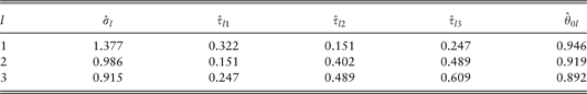
We randomly divide the data set into one estimation data set (75% of the 95668 customers), for estimation of the model parameters as described in Bühlmann & Gisler (Reference Bühlmann and Gisler2005) p. 185–186 or Englund et al. (Reference Englund, Gustafsson, Nielsen and Thuring2009), and one validation data set (the remaining 25% of the customers). The estimates of the model parameters, obtained from the estimation data set, are found in Table 1.
Table 1 Estimates of the model parameters, obtained from the estimation data set.
For the validation data set, we define the cross-sale product k to be any of {1, 2, 3} and define the existing product k′ to be any of the other products in {1, 2, 3} with k ≠ k′. Thereafter ![]() is estimated using (3), for every customer i in the validation data set, using the estimated model parameters in table 1 and by using that Fi ·k ′ has taken the observed individual values
is estimated using (3), for every customer i in the validation data set, using the estimated model parameters in table 1 and by using that Fi ·k ′ has taken the observed individual values ![]() , for every customer i in the validation data set, with respect to the existing product k′. Hence, we imagine only knowing about the a priori expected number of claims λi ·k ′ and the observed number of claims ni ·k ′, with respect to the existing product k′, in the validation data set. This is a very realistic situation for an insurance company aiming at cross-selling the i-th customer another insurance product k, by estimating specific model parameters, using a collateral data set, and thereafter evaluating the model with available customer specific information in order to assess (in this case) the customer's individual risk profile.
, for every customer i in the validation data set, with respect to the existing product k′. Hence, we imagine only knowing about the a priori expected number of claims λi ·k ′ and the observed number of claims ni ·k ′, with respect to the existing product k′, in the validation data set. This is a very realistic situation for an insurance company aiming at cross-selling the i-th customer another insurance product k, by estimating specific model parameters, using a collateral data set, and thereafter evaluating the model with available customer specific information in order to assess (in this case) the customer's individual risk profile.
Since we have the a priori expected number of claims λi ·k and the observed number of claims ni ·k available, for the customers in the validation data set, with respect to the cross-sale product k, we are able to evaluate if ![]() is a good estimator of the risk profile θik. It should be noted that since we have claims information, λi ·k and ni ·k with respect to the cross-sale product k, for every customer i in the validation data set, our imaginary cross-sale campaign has resulted in every customer accepting the cross-sale offer. This is of course unlikely in practice, where normally as few as 1 of 10 approached customers accept a cross-sale offer, but this is assumed in order not to obstruct the study. A more realistic study would be to incorporate a (possibly generalised linear) model for the cross-sale probability and analyse observed data from a cross-sale campaign, but this is outside the scope of the paper.
is a good estimator of the risk profile θik. It should be noted that since we have claims information, λi ·k and ni ·k with respect to the cross-sale product k, for every customer i in the validation data set, our imaginary cross-sale campaign has resulted in every customer accepting the cross-sale offer. This is of course unlikely in practice, where normally as few as 1 of 10 approached customers accept a cross-sale offer, but this is assumed in order not to obstruct the study. A more realistic study would be to incorporate a (possibly generalised linear) model for the cross-sale probability and analyse observed data from a cross-sale campaign, but this is outside the scope of the paper.
As stated in Section 3, we aim at cross-selling a product k to an expected profitable subset Φ* from a larger group of customers. We estimate θik with ![]() using (3), for the customers in the validation data set, order these by increasing
using (3), for the customers in the validation data set, order these by increasing ![]() (see (4)) and divide them into a number of equally sized sets Φm, with m = 1 ,…, M. We set M = 10 which gives
(see (4)) and divide them into a number of equally sized sets Φm, with m = 1 ,…, M. We set M = 10 which gives
The size of each set Φm is φm = 2, 382 for m = 1,…,10 and I = 23820 is here the number of customers in the validation data set. It is obvious that ![]() , see (5).
, see (5).
Figures 2–4 show ![]() and
and ![]() for the 10 sets Φ1,…,Φ10 for k = 1, k = 2 and k = 3, respectively. The risk profile
for the 10 sets Φ1,…,Φ10 for k = 1, k = 2 and k = 3, respectively. The risk profile ![]() is estimated using the model parameter estimates obtained from the estimation data set (see table 1) and the available customer specific information about λi ·k ′ and ni ·k ′ for customer i in the validation data set, with respect to one of the other products k′ ∈ {1,2,3} with k ≠ k′. From figures 2–4, it should be noted that the observed average profitability
is estimated using the model parameter estimates obtained from the estimation data set (see table 1) and the available customer specific information about λi ·k ′ and ni ·k ′ for customer i in the validation data set, with respect to one of the other products k′ ∈ {1,2,3} with k ≠ k′. From figures 2–4, it should be noted that the observed average profitability ![]() follows the expected average profitability
follows the expected average profitability ![]() nicely, which suggest that the estimator in (3) produces estimates of the risk profile θik close to the actual values.
nicely, which suggest that the estimator in (3) produces estimates of the risk profile θik close to the actual values.

Figure 2 Expected (filled dots) and observed (circles) average profitability for cross-selling of product k = 1, based on data from either product k′ = 2 or product k′ = 3.

Figure 3 Expected (filled dots) and observed (circles) average profitability for cross-selling of product k = 2, based on data from either product k′ = 1 or product k′ = 3.

Figure 4 Expected (filled dots) and observed (circles) average profitability for cross-selling of product k = 3, based on data from either product k′ = 1 or product k′ = 2.
As can be seen, from figures 2–4, different product combinations (of the cross-sale product k and the existing product k′) produces slightly different shapes of the expected average profitability as a function of the different subsets Φm, m = 1,…10. Comparing e.g. left and right hand sub-plot of figure 4, there is a larger spread between ![]() and
and ![]() for the product combination k = 3 and k′ = 2 than for product combination k = 3 and k′ = 1. This indicates that the estimator
for the product combination k = 3 and k′ = 2 than for product combination k = 3 and k′ = 1. This indicates that the estimator ![]() (based on available data from product k′ = 2) differentiates between expected profitable and expected unprofitable subsets Φm in a more effective way than the estimator
(based on available data from product k′ = 2) differentiates between expected profitable and expected unprofitable subsets Φm in a more effective way than the estimator ![]() (based on available data from product k′ = 1). Hence, available claims information for product k′ = 2 should be preferred over corresponding information from product k′ = 1, when selecting customers to cross-sale product k = 3 to. Similar comparisons can be made with respect to figure 2 and figure 3.
(based on available data from product k′ = 1). Hence, available claims information for product k′ = 2 should be preferred over corresponding information from product k′ = 1, when selecting customers to cross-sale product k = 3 to. Similar comparisons can be made with respect to figure 2 and figure 3.
A realistic situation, for an insurance company aiming at cross-selling a product k to its existing customers with a product k′, is to define a maximum number of customers to approach. The reason being limited resources for interacting with the customers, e.g. limited number of employees in the call centre. We replicate this situation by assuming that the maximum number of customers, which the insurance company has resources to approach, is φm = 2382 (i.e. the size of one of the subsets Φm) and the company should select the expected most profitable customers from its portfolio of existing customers. We assume that the portfolio of existing customers is the validation data set where individual claims information from the cross-sale product k is imagined unavailable. Since ![]() , the expected most profitable set of customers to approach is Φ1. The expected average profitability
, the expected most profitable set of customers to approach is Φ1. The expected average profitability ![]() as well as the observed average profitability
as well as the observed average profitability ![]() , for all combinations of k and k′, is shown in table 2. We assume that all of the 2382 imagined contacted customers accepted the offer of purchasing the cross-sale product k.
, for all combinations of k and k′, is shown in table 2. We assume that all of the 2382 imagined contacted customers accepted the offer of purchasing the cross-sale product k.
Table 2 Expected ![]() and observed
and observed ![]() average profitability in the expected most profitable cross-sale set Φ1. Also the corresponding minimum
average profitability in the expected most profitable cross-sale set Φ1. Also the corresponding minimum ![]() and maximum
and maximum ![]() values of estimated risk profiles are shown.
values of estimated risk profiles are shown.
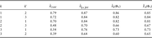
From table 2, the observed average profitability ![]() for the product combination (k = 2, k′ = 3) and (k = 3, k′ = 2) deserves special attention. For k = 2 and k′ = 3 an average profitability of
for the product combination (k = 2, k′ = 3) and (k = 3, k′ = 2) deserves special attention. For k = 2 and k′ = 3 an average profitability of ![]() is observed, interpreted as this set consists of customers with on average 33% less observed claims than a priori expected. The corresponding situation for k = 3 and k′ = 2 results in a set of customers with on average 36% less observed claims than a priori expected. This indicates not only that profitable selections are available but also that the correlation in claim occurrence is relatively high between the building product (k = 2) and the content product (k = 3), i.e. customers with reported number of claims lower than a priori expected for one of the products, suggests that a similar pattern can be expected with respect to the other. The smallest effect is shown for product k = 1, the set Φ1 consists of customers with on average between 15% and 16% less observed claims than expected.
is observed, interpreted as this set consists of customers with on average 33% less observed claims than a priori expected. The corresponding situation for k = 3 and k′ = 2 results in a set of customers with on average 36% less observed claims than a priori expected. This indicates not only that profitable selections are available but also that the correlation in claim occurrence is relatively high between the building product (k = 2) and the content product (k = 3), i.e. customers with reported number of claims lower than a priori expected for one of the products, suggests that a similar pattern can be expected with respect to the other. The smallest effect is shown for product k = 1, the set Φ1 consists of customers with on average between 15% and 16% less observed claims than expected.
5. Concluding remarks
This paper presents a method for identifying an expected profitable set of customers Φ*, to cross-sell to them an insurance product k, by estimating a customer specific latent risk profile θik using the customer specific available data for another insurance product k′. For the purpose, we consider a multivariate credibility estimator found in Englund et al. (Reference Englund, Gustafsson, Nielsen and Thuring2009) and investigate the effect of assuming that one (of two) insurance products is inactive (without available claims information) when estimating the latent risk profile θik. We also recognise that in order to estimate θik, estimates of certain model parameters have to be obtained from collateral data consisting of customers with both products k and k′ active, and whose characteristics are close to the characteristics of the customers for which an estimate of θik is sought after.
In Section 4 we have tested the proposed cross-sale method with a large data set from a Danish insurance company consisting of personal lines customers with 3 active insurance products (at the time of data collection). The data set is randomly divided into two data sets, where estimates of the model parameters are obtained from the estimation data set and a customer specific latent risk profile θik is estimated for every customer in the other validation data set. The estimate of the latent risk profile ![]() , for the cross-sale product k ∈ {1,2,3}, is obtained with the model parameters from the estimation data set and the available, customer specific, information about λi ·k ′ and ni ·k ′, in the validation data set, with respect to the existing product k′ ∈ {1,2,3}, with k ≠ k′.
, for the cross-sale product k ∈ {1,2,3}, is obtained with the model parameters from the estimation data set and the available, customer specific, information about λi ·k ′ and ni ·k ′, in the validation data set, with respect to the existing product k′ ∈ {1,2,3}, with k ≠ k′.
The observed average profitability ![]() for a set Φ of customers is close to the expected average profitability
for a set Φ of customers is close to the expected average profitability ![]() , with only few exceptions, as seen in figures 2, 3 and 4, which suggest that the estimators
, with only few exceptions, as seen in figures 2, 3 and 4, which suggest that the estimators ![]() (k ∈ {1,2,3} and k′ ∈ {1,2,3}, with k ≠ k′) would be useful in practice. However, the validation is performed using only a single data set and the method might give other results for other data sets, especially if the correlation in claim occurrence (between insurance products) is low. For the analysed Danish insurance data set, there are combinations of cross-sale product k and existing product k′ which perform better than others, especially the combinations (k = 2, k′ = 3) and (k = 3, k′ = 2) produce very profitable cross-sale selections with an observed average profitability as low as 0.64, which is interpreted as 36% less reported claims than a priori expected. This indicates a strong correlation between building claims (k = 2) and content claims (k = 3) and it is argued that an insurance company would be interested in directing cross-sale efforts towards customers with high profitability for one of these products but lacking the other one. Even though the effect is smaller when cross-selling motor insurance (k = 1), figure 2 and table 2 show that the proposed cross-sale method is able to identify a set of customers with 16% less claims than expected, which for a large insurance company translates into a considerable profit increase. The insurance company might also consider offering discounted premiums, on the cross-sale product k, to the customers in a set Φ*, to increase sales volume. In this case
(k ∈ {1,2,3} and k′ ∈ {1,2,3}, with k ≠ k′) would be useful in practice. However, the validation is performed using only a single data set and the method might give other results for other data sets, especially if the correlation in claim occurrence (between insurance products) is low. For the analysed Danish insurance data set, there are combinations of cross-sale product k and existing product k′ which perform better than others, especially the combinations (k = 2, k′ = 3) and (k = 3, k′ = 2) produce very profitable cross-sale selections with an observed average profitability as low as 0.64, which is interpreted as 36% less reported claims than a priori expected. This indicates a strong correlation between building claims (k = 2) and content claims (k = 3) and it is argued that an insurance company would be interested in directing cross-sale efforts towards customers with high profitability for one of these products but lacking the other one. Even though the effect is smaller when cross-selling motor insurance (k = 1), figure 2 and table 2 show that the proposed cross-sale method is able to identify a set of customers with 16% less claims than expected, which for a large insurance company translates into a considerable profit increase. The insurance company might also consider offering discounted premiums, on the cross-sale product k, to the customers in a set Φ*, to increase sales volume. In this case ![]() , for the customers i ∈ Φ*, can be used as a limit for how large the discount, for a specific customer i, is allowed to be.
, for the customers i ∈ Φ*, can be used as a limit for how large the discount, for a specific customer i, is allowed to be.


