


1. Introduction
Pension scheme deficits continue to be a cause of concern in the United Kingdom. There are several ways of measuring the shortfall of assets relative to liabilities, but an increasingly relevant measure is the cost of buyout. On this measure, there were sufficient assets to cover only 62% of buyout liabilities in 2015, and in the previous 10 years this figure has never risen above 68% (Pension Protection Fund, 2015). However, deficits are largely a historical issue – in other words, they relate to liabilities that have already been accrued.
At least as important are the costs for an employer that ongoing pension accrual continues to generate – and how that cost has changed over time. In addition, it is important to recognise not only how much these costs have risen, but also what has driven these costs. I therefore analyse the change in pension costs to identify the extent to which key drivers – discount rates, longevity and the benefits payable – have affected the change in cost. I also show the change in these costs in the context of other employment-related expenses, particularly National Insurance Contributions (NICs).
The answer to these questions is important, as it shows the impact that defined benefit (DB) accrual has on the cost of employment. In particular, it shows how the cost of employment has changed for an employer funding a defined benefit pension scheme compared with one providing a defined contribution arrangement. This is important because it demonstrates the extent to which defined benefit pensions are an additional burden to the employers that still provide them.
It is also important to recognise the relevance of defined benefit pension funding from another perspective – that is, how it affects the value of earnings that individuals receive. In other words, it is important to recognise how much the earnings of individuals have changed once the value of pension accrual is taken into account. This is important because the value of defined benefit pension accrual provides an indication of cost of an adequate retirement income – something that is relevant for individuals in defined contribution (DC) schemes.
Danzer & Dolton (2012) consider the value of pension accrual when they propose a measure of total reward which includes not just pay, but pensions and other benefits in kind. They go on to evaluate it as the present value of the sum of all these payments over an individual’s lifetime.
This issue of pension accrual in this context is also addressed in Sweeting (Reference Sweeting2008), which looks at the change in the cost and value of accrual from 1995 to 2005. This paper extends that work to 2015 and beyond, as well as improving the methodology.
Other authors have looked at the value of defined benefit accrual in the context of public and private sector pensions. All public sector schemes are defined benefitFootnote 1 , whilst private sector-defined benefit provision is continuing to decline in importance. Indeed, from 2004 to 2015, the number of active members of private sector defined benefit schemes fell from 3.6 million to 1.6 million. Furthermore, of the 1.6 million active members in private sector defined benefit schemes, only 0.6 million were in schemes or sections of schemes that were open to new members. However, for public sector defined benefit schemes, the number of active members rose from 5.0 million to 5.6 million over the same period (Office for National Statistics, 2015, 2016).
A common approach in this type of analysis is to look at the average level of pension provision in the public and private sector. Using this approach, Disney et al. (Reference Disney, Emmerson and Tetlow2009) find that the impact of defined benefit pensions for public sector employees is to make employment more valuable than for private sector employees even if the latter are members of defined benefit pension plans. This analysis controls for age, sex and education. The clear limitation of this analysis is that not all private sector workers are accruing defined benefit pensions.
Cribb & Emmerson (2016 Reference Cribb and Emmersona ) go further than Disney et al. (Reference Disney, Emmerson and Tetlow2009), controlling not just for age, sex and education, but also for experience and region. They carry out an examination of the impact of pensions on the pay of public and private sector workers, allowing for type of pension provision for those in the private sector, thus overcoming the main limitation in the work of Disney et al. Cribb and Emmerson value defined benefit pension accrual using the current unit method, which gives the change in discounted present value of the pension income from 1 year to the next, net of employee contributions. For defined contribution pensions, Cribb and Emmerson look not only at the level of contributions, but also at the returns received. This is used to give a view of the value of pension accrual in 2012 under a range of different scenarios. They then go on to look at the average pay differential between public and private sector workers over time, allowing for the average level and type of pension provision in each group. This analysis shows that public sector pay is significantly higher than private sector pay, even before allowing for pensions – and that pensions only increases this differential.
Whilst this analysis is useful from an aggregate standpoint, it does not explicitly address the question of the impact over time on an individual who is a member of a defined benefit rather than a defined contribution scheme. This is important because the decline in private sector defined benefit provision has been matched by the growth in private sector defined contribution provision. It is worth considering developments in defined contribution pensions further, as it is the contribution rates here against which the cost of defined benefit accrual should be compared.
The Office for National Statistics (2015, 2016) reports that over the period 2004–2015, active membership of occupational defined contribution schemes – that is, those defined contribution schemes set up by an employer under trust law – rose from 1.0 million to 3.9 million, although the bulk of this rise came as a result of the National Employment Savings Trust, which received a large number of members following the introduction of auto-enrolmentFootnote 2 . This is emphasised by the fact that active membership of defined contribution schemes grew from 1.2 million to 3.2 million between 2013 and 2014, the period during which auto-enrolment came into effect.
The process of auto-enrolment is being rolled out until February 2018Footnote 3 , so the growth of active membership in defined contribution plans can be expected to continue. Auto-enrolment is important because it includes a specification of the minimum level of contributions that must be paid. However, the minimum level of contributions allowed for by auto-enrolment is not large. Until April 2018, the minimum contribution is 2% of qualifying earnings – that is, earnings between the Lower Earnings Limit and the Upper Earnings Limit – of which the employer must pay at least 1% of qualifying earnings; the total contribution is expected to rise to 5%, with a minimum employer contribution of 2%, in April 2018; and from April 2019, it is proposed that the minimum will rise again to 8% of salaries and an employer minimum of 3% of salariesFootnote 4 . The 2018 levels are comparable with current levels of contribution to defined contribution schemes: the Office for National Statistics (2016) estimates that in 2015, members of open defined contribution schemes contributed 1.5% of salaries, with employers contributing 2.5% of salaries. Because these percentages relate to salaries rather than qualifying earnings, a direct comparison with auto-enrolment figures is not possible. The 2015 figures are lower even than those from 2014, where employees contributed 1.7% of salaries and employers contributed 2.9% of salaries (Office for National Statistics, 2015). These low rates are coincident with the introduction of auto-enrolment – in 2013, employees contributed 2.5% of salaries, with employers paying 6.0%. This might suggest that contribution rates for the newly auto-enrolled are at or close to legal minima. However, Cribb & Emmerson (2016 Reference Cribb and Emmersonb ) find that there is a large increase in contributions at the minimum levels, but also a substantial increase in the proportion of people with contributions well above the minimum.
One would therefore expect that auto-enrolment – particularly when higher contribution rates arrive – should result in larger pots for members of defined contribution schemes. But this does not necessarily mean that the level of benefits will be adequate. As mentioned above, the cost of defined benefit pension provision is a sensible benchmark against which defined contribution schemes can be measured. One comparison is of the contributions actually paid. the Office for National Statistics (2016) estimates that in 2015, members of open defined benefit schemes contributed 5% of salaries, with employers contributing 16.2% of salaries. However, these contribution rates reflect not just the cost of ongoing benefits, but also the deficit reduction contributions paid in respect of previously accrued benefits. Instead, it makes sense to calculate the cost of future benefits for a defined benefit pension scheme explicitly, as I do in this paper, and to compare it to the levels of contributions being made to defined contribution schemes.
2. Organisation of This Paper
First, I outline way in which I calculate the cost of pension accrual, in section 3. In this section, I describe both the methodology I use, and the assumptions that I make. In section 4, I calculate the change in earnings, and the appropriate allowance for NICs and for income tax. In section 5 I present my results. First, I give the total cost of accrual, before analysing the factors driving the year-to-year changes. I then look at the impact of defined benefit pension accrual on the cost of employment for a company, and then on the value of earnings to an employee.
3. Calculating the Cost of Pension Accrual
3.1. Overview
The cost of pension accrual is calculated as a proportion of salary. In this paper, I assume that the benefit accrued is one-sixtieth of earnings, with a retirement age of 65. I also assume that the nature of the benefit is final salary: in other words, the pension accrued in any year is revalued to retirement in line with the expected growth in earnings. However, for reasons discussed later, I also consider the change in the cost of accrual for members of career average revalued earnings (CARE) schemes, where pensions are increased prior to retirement in line with price inflation, subject to a maximum of 5% per annum over the period. The pension is then paid for the lifetime of the individual, with increases being paid in line with statutory minima. For simplicity, it is assumed that the individual accruing benefits is a man, that no spouse benefits are accrued, and that there is no guarantee period. The analysis is carried out on an annual basis, and the period covered in the main analysis is the 12-month period starting 31 March 1995 to the 12-month period starting 31 March 2015. These dates are chosen to coincide with the changes in tax years that start a few days later on 6 April and, thus, tax rates and bands. The discount and inflation rates as at the previous month end are used.
The cost of accrual as at 31 March 2015 can be used to calculate the impact of pensions for the 12-month period to 31 March 2016. However, it is interesting to consider the impact of interest rate changes in the light of the Brexit referendum, and also the potential move from statutory to conditional increases to pensions in payment.
On 23 June 2016, the United Kingdom voted to leave the European Union. In order to offset the impact of this decision on the UK economy, the Bank of England cut base rates to 0.25% and embarked on a policy of quantitative easing (QE). Research on the last programme of QE that ran from 2009 to 2012 indicates that long-term bond yields has been lowered by anything from 30 to 125 basis points (Meier, Reference Meier2009; Joyce et al., Reference Joyce, Lasaosa, Stevens and Tong2011; Breedon et al., Reference Bridges and Thomas2012; Bridges & Thomas, Reference Christensen and Rudebusch2012; Christensen & Rudebusch, 2012; Kapetanios et al., Reference Kapetanios, Mumtaz, Stevens and Theodoridis2012). More specific research on the term structure of changes, as well as the impact on real interest rates, shows that pension scheme liabilities had been significantly inflated by the Bank of England’s purchases (Sweeting et al., Reference Sweeting, Christie and Gladwyn2013). Given that long-term interest rates as at 30 September 2016 were significantly lower than they were as at 31 March 2016, it seems that the round of QE is having a similar impact. As such, I also look at the cost of accrual calculated on the 31 March 2015 basis, but using bond yields and expected inflation as at 31 March 2016 and 30 September 2016.
In a more recent development, it has been suggested that the guaranteed pensions in payment, whether at 5% Limited Price Indexation (LPI) or 2.5% LPI, could be replaced with conditional indexation (Cumbo, Reference Danzer and Dolton2016). This is a mechanism by which increases to pensions are paid only if there are sufficient funds; otherwise, pensions remain flat. It is straightforward to evaluate the impact of such a change on the cost of future accrual, so I look at how this would affect the estimated cost of accrual at 30 September 2016.
The cost of pension benefits is calculated by projecting into the future the payments arising from the year of pension accrual, and then discounting these payments back to give a present value. More precisely, the value at time 0 of a payment made at time t (where t=1,2,3 … and is measured in years) to a member of a final salary scheme currently aged x whose retirement age is 65 is c x,t , which is equal to
 $$c_{{x,t}} \, {\equals}\, \left\{ {\matrix{ {{1 \over {60}}{\times}{{l_{{x{\plus}t,t}} } \over {l_{{x,0}} }}{\times}{{e_{{65\, {\minus}\, x}} } \over {e_{0} }}{\times}{{i_{t}^{c} } \over {i_{{65\, {\minus}\, x}}^{c} }}{\times}\mathop \prod\limits_{j\, {\equals}\, 1}^t {1 \over {1{\plus}d_{j} }}} & \quad {{\rm if }\ \ t\geq 65\, {\minus}\, x} \cr {\hskip -130pt 0} & {{\rm otherwise}} \cr } } \right.$$
where l
x+t,t
is the projected population for age x+t and time t, so l
x+t,t
/l
x,0 is the probability of an individual aged x surviving to time t; e
t
the earnings index at time t used to revalue benefits before retirement;
 $i_{t}^{c} $
the capped price index used to increase benefits after retirement at time t – that is, the rate of change in the index is limited to some capped amount; and d
t
the spot discount rate for a term of t. The various price indices used are discussed in section 3.3; the discount rate is discussed in section 3.4; and earnings are discussed in section 3.5. A similar formula is used for members of CARE schemes:
$i_{t}^{c} $
the capped price index used to increase benefits after retirement at time t – that is, the rate of change in the index is limited to some capped amount; and d
t
the spot discount rate for a term of t. The various price indices used are discussed in section 3.3; the discount rate is discussed in section 3.4; and earnings are discussed in section 3.5. A similar formula is used for members of CARE schemes:
 $$c_{{x,t}} \, {\equals}\, \left\{ {\matrix{ {{1 \over {60}}{\times}{{l_{{x{\plus}t,t}} } \over {l_{{x,0}} }}{\times}\min \left[ {1.05^{{65\, {\minus}\, x}} ,{{i_{{65\, {\minus}\, x}} } \over {i_{0} }}} \right]{\times}{{i_{t}^{c} } \over {i_{{65\, {\minus}\, x}}^{c} }}{\times}\mathop \prod\limits_{j\, {\equals}\, 1}^t {1 \over {1{\plus}d_{j} }}} & \quad {{\rm if }\ \ t\geq 65\, {\minus}\, x} \cr {\hskip -190pt 0} & {{\rm otherwise}} \cr } } \right.$$
where all terms are as per equation (1), with the additional term i t being the price index at time t used to revalue benefits before retirement. The total cost of accrual for age x, per £1 of gross earnings, C x is obtained by summing the values of these individual cash flows:
 $$C_{x} \, {\equals}\, \mathop \sum\limits_{k\, {\equals}\, 1}^{120\, {\minus}\, x} c_{{x,k}} $$
The upper limit in this summation reflects the assumption that no individuals will live beyond 120. This is built into the longevity model used, which I describe in section 3.2. I further define the cost of accrual for an individual aged x evaluated at time t as C x,t . This can be used to derive the change in the cost of accrual over time, as
 $${\rm \Delta }C_{{x,t}} \, {\equals}\, {{C_{{x,t}} } \over {C_{{x,t\, {\minus}\, 1}} }}$$
A similar formula can be used to calculate the impact on the cost of accrual of longevity, benefit changes and interest rates. Let
 $C_{{x,t}}^{l} $
be the cost of accrual for an individual aged x evaluated at time t, but using the longevity data from t−1. The element of the change relating to longevity,
$C_{{x,t}}^{l} $
be the cost of accrual for an individual aged x evaluated at time t, but using the longevity data from t−1. The element of the change relating to longevity,
 ${\rm \Delta }C_{{x,t}}^{l} $
, is therefore
${\rm \Delta }C_{{x,t}}^{l} $
, is therefore
 $${\rm \Delta }C_{{x,t}}^{l} \, {\equals}\, {{C_{{x,t}} \, {\minus}\, C_{{x,t}}^{l} } \over {C_{{x,t\, {\minus}\, 1}} }}$$
Equivalent expressions can be derived for the impact of benefit changes and interest rates.
3.2. The longevity model
Improving life expectancy clearly has an impact on the cost of future pension accrual. There are two components of longevity that are of interest here. The first is the expected change in longevity. When moving from time t to time t+1, one would expect the cost of accrual to increase because of anticipated improvements in life expectancy. However, if the change in longevity is different from than anticipated, then this will clearly have an additional impact on the cost of pension accrual.
In modelling life expectancy, I assume that at any time t, information on mortality rates will be available only up to time t−2. The mortality data used are central rate of mortality for England and Wales males aged 20–100, from the Human Mortality Database (2016). The natural logarithm of mortality rates is extrapolated linearly from age 101 to 120, based on data from ages 81 to 100. I then take data from t−21 to t−2 and ages 20–120, and apply singular value decomposition to the data, as described by Lee & Carter (Reference Lee and Carter1992). I then fit a linear function to the time component, and project this forward. Applying this to the age components gives projected central mortality rates for times t−1 onward. Each central mortality rate m x,t is converted to an initial mortality rate, q x,t . For age 20, the following formula is used:
 $$q_{{20,t}} \, {\equals}\, m_{{20,t}} \left[ {{{1{\plus}\left( {1\!/\!2} \right)m_{{21,t}} } \over {1{\plus}\left( {1\,/\,12} \right)\left( {7m_{{20,t}} {\plus}5m_{{21,t}} } \right){\plus}\left( {1\!/\!3} \right)m_{{20,t}} m_{{21,t}} }}} \right]$$
for ages 21–100, the following approximation is used:
 $$q_{{x,t}} \, {\equals}\, m_{{x,t}} \left[ {{{1{\plus}\left( {1\!/\!2} \right)m_{{x\, {\minus}\, 1,t}} } \over {1{\plus}\left( {5\,/\,12} \right)\left( {m_{{x,t}} \, {\minus}\, m_{{x\, {\minus}\, 1,t}} } \right)\, {\minus}\, \left( {1\!/\!6} \right)m_{{x,t}} m_{{x\, {\minus}\, 1,t}} }}} \right]$$
and for ages over 100, the following approximation is used:
 $$q_{{x,t}} \, {\equals}\, {{m_{{x,t}} } \over {1{\plus}m_{{x,t}} }}$$
Each year, a new year of mortality information is assumed to become available, so the projected mortality is recalculated. This approach differs from that used in Sweeting (Reference Sweeting2008), where I estimated changes dues to mortality costs using mortality tables published by the CMI Bureau. Because updates to these tables are produced infrequently, the impact of longevity improvements can appear uneven. Furthermore, because they are produced only some years after the period of analysis, the impact of longevity improvements is not recognised until a significant period after it has been felt by the scheme.
As well as allowing the cost of the defined benefit accrual to be calculated, I am also able to isolate the impact on the cost of changes in longevity.
3.3. Benefit changes
A key part of the analysis is the impact on the cost of pension accrual of the benefit changes that have occurred due to legislation. The first of these was the requirement to provide increases to pensions in payment in line with the Retail Prices Index (RPI), subject to a maximum of 5% per annum, from 5 April 1997. This is known as 5% Limited Price Indexation, or 5% LPI. Prior to 5 April 1997, no increases to pensions in payment were required unless a scheme was contracted out from the State Earnings-Related Pension Scheme. From April 2005, this minimum requirement was reduced, with the cap being cut to 2.5% per annum, giving 2.5% LPI. In terms of
 $i_{t}^{c} $
, this means that if, for example, the index is being considered at a time when 2.5% LPI is in force, the annual change in
$i_{t}^{c} $
, this means that if, for example, the index is being considered at a time when 2.5% LPI is in force, the annual change in
 $i_{t}^{c} $
cannot exceed 2.5% even if the change in RPI is >2.5%.
$i_{t}^{c} $
cannot exceed 2.5% even if the change in RPI is >2.5%.
From 5 April 2011 the rate of inflation used in the calculation of benefits was changed from the RPI to the Consumer Prices Index (CPI). This applies to both the rate underlying the 5% LPI increases to pensions in payment, and also to the increases to pensions in the period before retirement for members of CARE schemes. As stated in the section 3.1, the pension accrued in any year is revalued to retirement in line with price inflation, subject to a maximum of 5% per annum over the period. Before 5 April 2011, this measure of inflation was RPI; after this date it was CPI.
As with the longevity cost, the change in the minimum benefits allows me not only to calculate the change in the cost of benefit accrual, but also to isolate the impact on benefit accrual of the change in the minimum benefits payable.
In practice, an individual may have experienced benefit changes over the last two decades other than those dictated by legislation. Key amongst these is the change to a CARE basis from a final salary arrangement. Whilst the former allows for pensions to increase up to retirement in line with prices, the latter allows for an increase in line with salaries. The impact of this change depends on the difference between future salary and price inflation, and the age at which any change occurs, but an idea of the impact can be gauged by considering the change in the cost of final salary and CARE accrual over the period. Another potential change is a change to the retirement age, which again could take many forms. As such, I look at the order of magnitude that such changes might bring but they do not form part of the central analysis.
3.4. Interest rate changes
Cribb & Emmerson (2016 Reference Cribb and Emmersona ) make a key simplification in their model of pension costs, in that they assume a real discount rate of 3% per annum. This simplification is appropriate for single-period cross-sectional analysis. However, as I show in this paper, the change in discount rate has been an important factor in the changing value of defined benefit pensions.
The discount rate has more than one component. First, there are the inflation rates used to project benefits. Even if the benefit structure is not changing, the assumed rate of inflation by whatever measure is appropriate will develop over time. For RPI, the assumed rate of inflation is taken from the Bank of England’s implied inflation spot curve. This is calculated from the Bank of England’s nominal and real government bond spot curves.
All index-linked UK government bonds pay coupons based on RPI. As such, information on the CPI spot curve is harder to find. I therefore approximate it by deducting the average difference between historical RPI and CPI for the 10 years before the calculation date from the implied RPI inflation spot curve.
The projected cash flows are discounted using the spot rate on the UK nominal government bond yield curve at the appropriate term, as calculated by the Bank of England, plus a risk premium. The risk premium is 1% per annum, which is consistent with the difference between the median single effective discount rate and the Bank of England 20-year nominal spot rate observed by the Pensions Regulator (2016) from 2005 to 2014.
3.5. Projected earnings changes
A key assumption used to assess the cost of a defined benefit pension is the rate at which earnings increase before retirement. For this assumption, I add the average difference between historical earnings and historical RPI for the 10 years before the calculation date to the implied RPI inflation spot curve. This calculation itself yields some interesting results. As Figure 1 shows, historical real earnings increases have fallen significantly over the last 20 years, to the extent that real earnings growth relative to RPI is negative, and relative to CPI is around zero. This means that for calculations made as at 2014 or later, the estimate of future salary inflation is around the same as the estimate for future CPI inflation. This could also be used to estimate the impact over time of moving from a final salary scheme to a CARE arrangement.
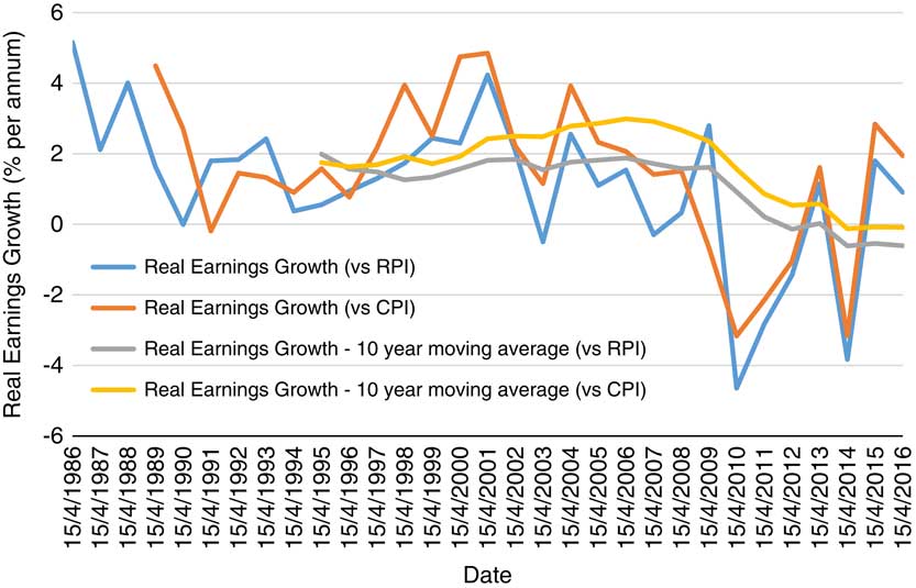
Figure 1 Historical real earnings growth. Source: Office for National Statistics, author’s calculations. RPI, Retail Prices Index; CPI, Consumer Prices Index.
4. Calculating the Change in Earnings
Before looking at the impact of pensions accrual on earnings, I first look at how earnings have themselves changed – both from the employer’s and the employee’s point of view. From the employer’s point of view, I compare
-
∙ gross earnings excluding pensions;
-
∙ gross earnings plus employer NICs; and
-
∙ gross earnings plus employer NICs plus defined benefit pension accrual.
From the employee’s point of view, I compare
-
∙ gross earnings excluding pensions;
-
∙ gross earnings less employee NICs and income tax; and
-
∙ gross earnings less employee NICs and income tax plus defined benefit pension accrual.
Initially, I define gross earnings as UK Private Sector Average Weekly Earnings from January 2000, and the UK Private Sector Average Earnings Index before this, both on a seasonally adjusted basis and including bonuses. As these series overlap, I am able to construct a continuous series of annual earnings for the full period of analysis. Annual figures for each 12-month period running from April to the following March are calculated by converting the weekly earnings figure for each month to a monthly figure, and then aggregating over the 12 months. The gross earnings series for the 12-month period t is G t . The percentage change in G t is then defined as
 $${\rm \Delta }G_{t} \, {\equals}\, {{G_{t} } \over {G_{{t\, {\minus}\, 1}} }}\, {\minus}\, 1$$
To determine the change in the total cost to the employer before pensions, which I denote
 ${\rm \Delta }N_{t}^{{er}} $
, employer NICs,
${\rm \Delta }N_{t}^{{er}} $
, employer NICs,
 $NIC_{t}^{{er}} $
, must be added to the numerator and denominator of (8):
$NIC_{t}^{{er}} $
, must be added to the numerator and denominator of (8):
 $${\rm \Delta }N_{t}^{{er}} \, {\equals}\, {{G_{t} {\plus}NIC_{t}^{{er}} } \over {G_{{t\, {\minus}\, 1}} {\plus}NIC_{{t\, {\minus}\, 1}}^{{er}} }}\, {\minus}\, 1$$
The change in net earnings including the cost of pension accrual from the employer’s point of view for an individual aged x for the year to time t is
 ${\rm \Delta }T_{{x,t}}^{{er}} $
, defined as
${\rm \Delta }T_{{x,t}}^{{er}} $
, defined as
 $${\rm \Delta }T_{{x,t}}^{{er}} \, {\equals}\, {{G_{t} {\plus}NIC_{t}^{{er}} {\plus}\left( {G_{t} {\times}C_{{x,t}} } \right)} \over {G_{{t\, {\minus}\, 1}} {\plus}NIC_{{t\, {\minus}\, 1}}^{{er}} {\plus}\left( {G_{{t\, {\minus}\, 1}} {\times}C_{{x,t\, {\minus}\, 1}} } \right)}}\, {\minus}\, 1$$
where C x,t is the cost of accruing an extra year’s pension per £1 of gross earnings for in individual aged x at time t. Note that this is the only earnings measure where age is relevant – in other words, I do not allow for any change in gross earnings by age.
From an employee’s point of view, the calculation is similar, except that NICs are a deduction rather than an addition, and that they are deducted along with income tax. Here, the change in net earnings excluding pension accrual is
 ${\rm \Delta }N_{t}^{{ee}} $
, defined as
${\rm \Delta }N_{t}^{{ee}} $
, defined as
 $${\rm \Delta }N_{t}^{{ee}} \, {\equals}\, {{G_{t} \, {\minus}\, NIC_{t}^{{ee}} \, {\minus}\, IT_{t}^{{ee}} } \over {G_{{t\, {\minus}\, 1}} \, {\minus}\, NIC_{{t\, {\minus}\, 1}}^{{ee}} \, {\minus}\, IT_{{t\, {\minus}\, 1}}^{{ee}} }}\, {\minus}\, 1$$
where
 $NIC_{t}^{{ee}} $
represents employee NICs, and
$NIC_{t}^{{ee}} $
represents employee NICs, and
 $IT_{t}^{{ee}} $
the income tax payable in year t. The change in net earnings including the cost of pension accrual from the employee’s point of view is
$IT_{t}^{{ee}} $
the income tax payable in year t. The change in net earnings including the cost of pension accrual from the employee’s point of view is
 ${\rm \Delta }T_{{x,t}}^{{ee}} $
, defined as
${\rm \Delta }T_{{x,t}}^{{ee}} $
, defined as
 $${\rm \Delta }T_{{x,t}}^{{ee}} \, {\equals}\, {{G_{t} \, {\minus}\, NIC_{t}^{{ee}} \, {\minus}\, IT_{t}^{{ee}} {\plus}\left( {G_{t} {\times}C_{{x,t}} } \right)} \over {G_{{t\, {\minus}\, 1}} \, {\minus}\, NIC_{{t\, {\minus}\, 1}}^{{ee}} \, {\minus}\, IT_{{t\, {\minus}\, 1}}^{{ee}} {\plus}\left( {G_{{t\, {\minus}\, 1}} {\times}C_{{x,t\, {\minus}\, 1}} } \right)}}\, {\minus}\, 1$$
For both employee and employer NICS, I assume that there is no contracting-out of the State Earnings-Related Pension Scheme of State Second Pension.
5. Results
5.1. Total cost of accrual
First, I look at the change in the cost of pension accrual. As discussed in section 3.1, I consider the 12-month period starting 31 March 1995 to the 12-month period starting 31 March 2015, but also look at the cost of accrual calculated on the 31 March 2015 basis, using bond yields and expected inflation as at 31 March 2016 and 30 September 2016. These results are given in Figure 2 for a 40-year-old male with a retirement age of 65, assuming a discount rate of UK government bonds plus 1% per annum, both as a member of a final salary scheme and a CARE arrangement.
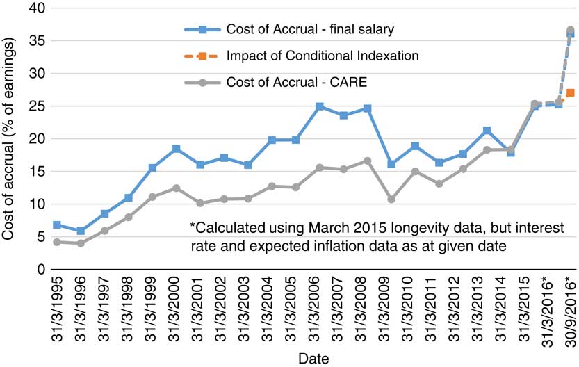
Figure 2 Accrual rate for a 40-year-old male pension scheme member. Source: Bank of England, Office for National Statistics, author’s calculations. CARE, career average revalued earnings.
This shows that in March 1995, the cost of accrual for a member of a final salary scheme was only 6.8% of earnings, dropping slightly the following year to 5.9% of earnings. The cost of accrual then grew steadily to the period commencing 31 March 2000, peaking at 18.5%. It then fell back slightly, before rising steadily up until 24.9% for the period commencing 31 March 2006. March 2009 saw a sharp drop back to 16.1%. The cost of accrual then rose gradually until March 2013, reaching 21.3%. There was a small 1-year drop, but after that the cost rose significantly in March 2015 to 25.0% of earnings, and again in September 2016 to 36.1% of earnings. Interestingly, whilst conditional indexation would cut the cost of accrual significantly, it would still leave it at its highest ever level – 27.0% of earnings for the period commencing 30 September 2016.
It is interesting to contrast the change in cost for a final salary member with that of a CARE beneficiary. Whilst the broad patterns are similar, the initial cost of a CARE pension is far lower, at 4.2% of salary. Up until 2008, real earnings growth means that the cost of final salary provision accelerates away from the cost of a CARE pension, as this growth is used to project future changes to real earnings. However, after this period, the impact of lower and ultimately negative real earnings growth sees the cost of a CARE pension actually overtaking that of a final salary pension by a small margin.
In fact, if we concentrate on the 10 years from 2005 to 2015 – the decade following the analysis in Sweeting (Reference Sweeting2008), we can see that after an increase in the period from 2005 to 2006, the cost of accrual for a final salary scheme has barely chanced (from 24.9% in 2006 to 25.0% in 2015). This contrasts with the change in the cost of accrual for a CARE scheme (from 15.6% in 2006 to 25.4% in 2015).
It should be clear that the assumption for real earnings growth is key here. In fact, for the period 2006–2015, the fall in the real earnings growth assumption negates the impact of all of the factors causing the rise apparent in the cost of CARE accrual. If a higher figure is used than that suggested here – essentially no real earnings growth from 2014 onwards, then the cost of providing a final salary pension will inevitably be greater.
For the remaining analysis, I look only at the cost of final salary accrual.
5.2. Components of accrual cost
The three components of the change in the cost of accrual – benefits, longevity and interest rates (including projected price inflation and earnings growth) – are described above, as is their calculation. Because the sum of each of the three components leaves a rounding error, I allocate the error to each of the three components in proportion to the size of each component. The results are shown in Figure 3.

Figure 3 Components of the change in the accrual rate for a 40-year-old male pension scheme member. Source: Bank of England, Office for National Statistics, author’s calculations.
Longevity increases have been a reasonably constant source of increasing pension costs. Some years have been worse than others: 2006 saw longevity contributing a 0.6% of earnings increase in the cost of accrual, whilst the average was only 0.3% per annum. The same average applies to the 10 years from 2005 to 2015, the decade following the analysis of Sweeting (Reference Sweeting2008). This variation largely reflects unexpected increases, rather than the variation arising from a population whose longevity is expected to improve. Overall, though, this 0.3% increase is small compared to the 0.9% increase arising from interest rates, which I discuss later.
The impact of the change in benefits has been, on average, small: it accounts for an increase in the cost of accrual of 2.2% of earnings from 1996 to 1997, when 5% LPI was introduced, and then a drop of 0.1% of earnings when 5% LPI was replaced by 2.5% LPI in 2005. The drop here was small because expected RPI inflation was not significantly >2.5%. This also means that the impact of benefit changes for a final salary scheme after 2005 is nil. Interestingly, if this analysis is repeated for a CARE scheme, there is an additional, larger fall in 2011 – equivalent to 2.3% of the cost of accrual – when RPI is replaced with CPI. This is because for a CARE scheme, increases both before and after retirement are affected, and the impact on pre-retirement increases is significant; however, by the time of this change, implied inflation on both an RPI and a CPI basis was >2.5% at all terms, so the change in inflation definition had no impact on the projected value of post-retirement component of benefits.
The suggested move to conditional indexation for pensions in payment would cause a much bigger drop in the cost of accrual: 9.6% of earnings. This assumes that conditional indexation would mean that there would be no guaranteed increases in benefits in payment. The change in cost is so high compared to the introduction of 5% LPI because long-term interest rates are so low now compared with 20 years ago. Figure 4, which shows the 20-year spot rate for nominal UK government bonds and for implied RPI inflation, demonstrates this clearly. This means that the present value of a change in future increases is correspondingly higher.

Figure 4 Twenty-year government bond yield and implied Retail Prices Index inflation rate. Source: Bank of England.
Figure 4 also helps to explain the change in the cost of accrual due to nominal government bond yields and implied inflation, which together with assumed earnings increases I refer to as interest rates. Both bond yields and implied inflation fell sharply from 1996 to 1999, with nominal rates falling more than implied inflation. This did lead to some noticeable increases in the cost of accrual, contributing to an increase of 2.3% of earnings in 1998, 4.3% in 1999 and 2.6% in 2000. However, because the 20-year bond yield in 1999 was still relatively high – at least when compared with the current yield – the impact was not catastrophic.
The combination of a rise in bond yields and a fall in implied inflation in 2001 led to a fall in the cost of accrual attributable to interest rates of 2.6% of earnings. Changes were smaller for a few years until interest rates contributed to a rise in the cost of accrual of 3.5% of earnings in 2004 and 4.5% of earnings in 2006 – this time, a fall in bond yields coincided with a rise in implied inflation. The next big change was in 2009. Although bond yields fell, implied inflation fell further, leading to a fall in the cost of accrual of 8.8% of earnings. A period of increased volatility followed. However, the next significant change happened in 2015, when falling bond yields added 7.0% of earnings to the cost of accrual, but even this was dwarfed by the fall in yields following the Brexit referendum: between March and September 2016, the fall in government bond yields added a further 10.9% of earnings to the cost of accrual on an annualised basis.
The average change in the cost of accrual due to interest rates for a final salary scheme member was 0.5% of earnings per annum for the period 1995–2015. This contrasts with an average of 0.9% of earnings for a CARE scheme. When considering the period 2005–2015, the difference is even more stark: 0.2% per annum for final salary versus 1.3% for CARE, with only the 2005–2006 observation keeping the final salary figure positive. This difference is purely down to the drop in projected real salary inflation. In other words, if it were not for this drop in real salary inflation, the change in interest rates would have had a far greater effect in the period 2005–2015 than in 1995–2005.
5.3. The cost of defined benefit pensions to employers
Having analysed not only the changes in the cost of accrual but also the drivers of these changes, I can now consider the impact of this cost on remuneration. First, however, it is worth looking at how remuneration has changed before allowing for pensions. If we concentrate on private sector earnings, we can easily see the impact of adding NICs to employer costs, as indicated in Figure 5. This shows the growth in earnings cost for individual earning one, two, four and eight times average earnings. The differences arise because of the differences in NIC rates and bands. It is clear here that the cost of employing people of all earnings levels has increased as a proportion of gross earnings.
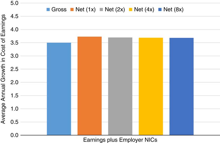
Figure 5 Average annual growth in net and gross cost of earnings, private sector including bonuses, seasonally adjusted, 1996–2016. Source: Office for National Statistics (Average Weekly Earnings from January 2000; constructed series using the Average Earnings Index before this), HM Revenue & Customs, author’s calculations. NICs, National Insurance Contributions.
Focussing on the net earnings at the average level, I then consider the difference between the cost of employing an individual in a defined contribution scheme and a defined benefit scheme. According to the Office for National Statistics (2015), members contribute on average 5% of earnings to private sector defined benefit pension schemes. The Office for National Statistics (2003) also indicate that employee contributions to contributory defined benefit schemes have been at or around this level since at least 2000. This amount must therefore be deducted from the cost of accrual, as it is a cost borne by the employee rather than the employer.
Until 2014, employer contributions to defined contribution schemes had also remained relatively stable, at around 6% of earnings. As outlined in section 1.3, employer contribution rates dropped considerably at this point, following the introduction of auto-enrolment. Since this drop in the average contribution rate is due to the addition of a heterogeneous population, and because the analysis is intended to be about the cost of defined benefit accrual rather than defined contribution provision, I assume a constant employer contribution of 6% of earnings for members of defined contribution schemes. In Figure 5, I therefore show three series for a 40-year-old individual on average earnings: the total cost of employment excluding pensions; the total cost of employment including a 6% contribution to a defined contribution scheme; and the total cost of employment including the cost of accrual for a defined benefit scheme, net of a 5% employee contribution.
There are two key features in Figure 6. First, the cost of employing a worker and providing a defined benefit pension has grown consistently more quickly than the cost of employing someone in a defined contribution scheme. To be precise, the average increase for a defined benefit employee was 4.7% per annum over the last 20 years, compared with 3.7% per annum for a defined contribution employee – a difference of 1.0% per annum. Most of this difference occurred over the period 1995–2005 – the average increase from 2005 to 2015 was only 0.5% per annum. However, it is also interesting to note that until 1999–2000, it was actually more expensive to have an employee in a defined contribution scheme than to provide membership of a defined benefit scheme.

Figure 6 Average annual growth in cost of average earnings, private sector including bonuses, seasonally adjusted, allowing for pensions, 1996–2016. Source: Office for National Statistics (Average Weekly Earnings from January 2000; constructed series using the Average Earnings Index before this), HM Revenue & Customs, author’s calculations. NICs, National Insurance Contributions.
5.4. The value of defined benefit pensions to employees
Moving onto the value of defined benefit pensions for employees, I first look at earnings net of employee NICs and income tax. It is clear from Figure 7 that there has been a significant move to increase redistribution, with net pay for the least well-paid increasing relative to gross earnings, and the opposite happening for the most well-off. Clearly, there is no guarantee that the net income for an individual would have increased by more or less than the average, but this does at least indicate a redistributive policy.
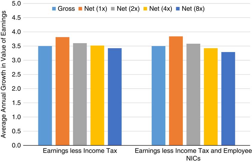
Figure 7 Average annual growth in net and gross value of private sector earnings, including bonuses, seasonally adjusted, 1996–2016. Source: Office for National Statistics (Average Weekly Earnings from January 2000; constructed series using the Average Earnings Index before this), HM Revenue & Customs, author’s calculations. NICs, National Insurance Contributions.
When looking at the value of accrual in Figure 8, I again concentrate on a 40-year-old individual on average earnings with a retirement age of 65. The result, unsurprisingly, has a similar profile to employer costs. The results are similar numerically as well – the average increase in earnings for a defined benefit employee was 4.8% per annum over the last 20 years, compared with 3.8% per annum for a defined contribution employee – again, a difference of 1.0% per annum. This too falls to 0.5% per annum if the period of 2005–2015 is considered.

Figure 8 Average annual growth in the value of average private sector earnings, including bonuses, seasonally adjusted, allowing for pensions, 1996–2016. Source: Office for National Statistics (Average Weekly Earnings from January 2000; constructed series using the Average Earnings Index before this), HM Revenue & Customs, author’s calculations. NICs, National Insurance Contributions.
6. Conclusion
The cost of employing a member of a final salary defined benefit pension scheme has outpaced the cost of employing someone in a defined contribution arrangement over the last 20 years. From 1996 to 2016, the difference in the total cost has been some 1.0% of earnings per annum. When looking instead from an employee’s point of view, the difference in change in the value of a defined benefit scheme relative to a defined contribution arrangement is the same – around 1.0% of earnings per annum. This means that allowing for an employee contribution of 5% of earnings, the employer’s cost of accrual grew from 1.8% of earnings in March 1995 (when the total cost was only 6.8% of earnings) to 20.0% of earnings in March 2015. As such, having employees who are still accruing defined benefit pensions has resulted in a growing financial burden for firms in this position. Much of the increase in cost and value took place over the period 1995–2005, with the average increase being only 0.5% higher for the period 2005–2015.
The average impact of interest rate changes on the change in the cost of accrual is 0.5% per annum. This is significantly more than the average impact of longevity improvements, which is 0.3% per annum. Both of these have added to the total cost, as has have changes to benefits, by around 0.1% per annum on average. The impact of interest rate changes has been moderated by the fall in real earnings. This can be seen by considering the impact of interest rate changes on the cost of accrual in a CARE scheme, which itself exceeded 0.9% per annum on average. The change from RPI to CPI also had an impact on CARE schemes by reducing the cost of accrual by 2.3%, wiping out the increase in cost due to benefit changes seen with final salary schemes.
Looking only at changes in interest rates, the change in cost from March 2015 to March 2016 was small, with the estimated cost of accrual to the employer rising only slightly, to 20.2%. However, following the Brexit vote and the subsequent reintroduction of QE, the estimated cost of accrual has risen to 31.1% as at September 2016.
If the current 2.5% LPI increases to pensions in payment were removed and replaced with conditional indexation, the cost of accrual for the employer would fall back to 22.0%.
The total cost of defined benefit accrual – including employee contributions – is therefore 36.1% of earnings as at September 2016, a number that would fall to 27.0% of earnings 2.5% LPI increases were removed. Contrast this with current payments to defined contribution schemes, which in 2015 stood at 4.0% of earnings, of which employers contributed 2.5%. It is likely that these figures are depressed by the large number of newly auto-enrolled members. But even before auto-enrolment, the total contribution rate to defined contribution schemes was only 8.5%, with employers paying 6.0%. This is marginally above the maximum auto-enrolment level that will be reached in April 2019, of 8% of earnings, with employers paying at least 3% – less than a third of the amount needed to match even a non-increasing defined benefit pension.
If we remain in a low growth, low interest rate environment, contributions to defined contribution schemes will need to rise sharply. If they do not, individuals relying on these schemes will reach retirement with inadequate assets and very uncertain futures – and the only group able to support them will be taxpayers.
Acknowledgment
The author would like to thank the reviewers of this article for their helpful observations.


