


1 Introduction
Disability insurance is a form of insurance payable to policyholders who are unable to work either permanently or for an extended time period, due to some impairment. There can be a significant delay, called a recording lag, between the date an impairment occurred (the incurred date) and the date on which a valid claim is recorded on the insurer's administrative system. The lag can be broken down into two parts:
(i) the time between the incurred date and the date on which a claim is received for consideration by the insurer. This delay can be due to a waiting period in the policy or uncertainty on the part of the insured on whether their current incapacity is temporary or not;
(ii) the time between the initial consideration date and the date on which the valid claim is recorded on the insurer's administrative system. This delay can be due to the time taken to assess both the validity of the claim and the extent of the work incapacity.
The insurer must take the recording lag into account when calculating reserves for claims which are incurred but not recorded. This prediction of incurred but not recorded claims is an important problem for the insurer. In disability insurance, it seems intuitive that claims experience should be linked to economic conditions; it is generally observed that many disability claims are a choice not to participate in the workforce, and the size and prospects of the workforce are affected by economic conditions. There are arguments as to the exact impact of the economic conditions, as highlighted in Schriek & Lewis (Reference Schriek and Lewis2010, Section 2). For example, there are arguments that disability rates should increase as the economy declines and other arguments that disability rates should increase as the economy booms. Studies have shown both these effects in different countries (see Schriek & Lewis Reference Schriek and Lewis2010, Section 2 for references). Whatever the precise impact on individual policyholders in a particular industry sector or country, the broad message is that changes in economic conditions should be reflected by changes in the disability experience. For this reason, we model the development of incurred but not recorded claims using economic factors in addition to the information gained from the past evolution of claims. Furthermore, we might expect that there is a delay before changes in economic conditions affect policyholder behaviour, since it takes time for industry and the policyholders to recognize the effects of a different economic environment. For claims prediction, this means that we may be able to use economic indicators observed in the past, for example one year ago, in order to improve the prediction of the claims development.
The use of economic indicators for the prediction of disability claims has been examined through linear regression in two papers. In Schriek & Lewis (Reference Schriek and Lewis2010), a linear regression of South African disability rates against various economic indicators is performed, with the goal of finding if there is a link between disability claims incidence and the state of the economy. They find that unemployment and consumer confidence indicators are strongly correlated with the disability experience. In König et al. (Reference König, Weber and Wüthrich2011), a Poisson model is applied in a Bayesian framework to Swiss data for the purposes of claim prediction. A strong correlation between the posterior mean of one of the fitted model parameters and the spread of corporate bonds over government bonds is found.
However, König et al. (Reference König, Weber and Wüthrich2011) do not incorporate a stochastic model of the economic indicators into the claims prediction model. Consequently, while their model is simple, it is not helpful for the quantification of prediction uncertainty, which is a drawback from a risk management perspective. In particular, their approach was to develop a Bayesian claims prediction model independently of the chosen economic indicator. Then the posterior mean of a parameter of the fitted model was linearly regressed against the economic indicator. If we use the resultant linear relationship to predict future claims then, as we are forced to consider only posterior means, we lose the powerful Bayesian predictive distribution and thus are unable to quantify prediction uncertainty.
The primary aim in this paper is to propose a Bayesian model which overcomes this limitation and hence allow us to
(i) justify the findings in König et al. (Reference König, Weber and Wüthrich2011);
(ii) stochastically project the economic indicators into the future;
(iii) consistently predict disability rates within the model; and
(iv) quantify prediction uncertainty.
The model we propose makes the chosen economic indicator an integral part of the Bayesian model, and thus melds both insurance information and economic information into the model in a natural way. We allow one of the model parameters to be a function of the economic indicator and choose a stochastic model for the future development of the economic indicator. Together, these assumptions enable us to obtain the full predictive distribution of the future claims, allowing for the impact of the economic indicator on the development of the claims. We can use the predictive distribution to calculate statistics of the future claims, calculate risk measures, such as value-at-risk or expected shortfall, and do more sophisticated analyses, for example applying extreme value theory to estimate the upper tail of the numbers of claims. We are not constrained to the use of the posterior means of the parameters in the prediction of claims, as in König et al. (Reference König, Weber and Wüthrich2011). We use the claims data from König et al. (Reference König, Weber and Wüthrich2011), which is income protection disability insurance for both temporary and permanent disability claims, with a minimum waiting period of three months. Our analysis found that the disability experience is strongly linked to the spread observed 1.25 years ago of corporate bond yields over government bond yields, which supports the findings of König et al. (Reference König, Weber and Wüthrich2011). We also examined an unemployment indicator, but we did not find it to be helpful for claims prediction.
The idea of directly incorporating an economic indicator into a Bayesian model for claims prediction is new. Although we use a specific set of claims data to illustrate our model, our approach can be applied to other claims data where there are solid reasons for assuming that the claims are affected by economic indicators, e.g. inflation. We emphasise the importance of a well-founded argument for assuming a link between the data and the chosen indicator.
2 Notation
An annual summary of the disability claims data that we work with is shown in Table 1. The data corresponds to the calendar years 1997 to 2008 and concerns only claims for which a disability payment will eventually be made. The data ![]() is shown as a claims development table, where the time period in which the claim was incurred is shown vertically and the lag before it was recorded on the insurer's administrative system is shown horizontally. The lower triangle is empty since this corresponds to claims which have been incurred but have not yet been recorded on the insurer's administrative system. The right-most column shows the number of insured lives in each incurred period. Our aim is to find a suitable model for the incurred but not recorded claims so that we can predict the lower triangle.
is shown as a claims development table, where the time period in which the claim was incurred is shown vertically and the lag before it was recorded on the insurer's administrative system is shown horizontally. The lower triangle is empty since this corresponds to claims which have been incurred but have not yet been recorded on the insurer's administrative system. The right-most column shows the number of insured lives in each incurred period. Our aim is to find a suitable model for the incurred but not recorded claims so that we can predict the lower triangle.
Table 1 Claims development table (annual figures).
We denote by Ni,j the number of claims which were incurred in period i and were recorded by the insurer j time periods later. Thus in Table 1, N 5,1 = 5933 is the number of claims which were incurred in calendar year 2002 and were recorded in calendar year 2003 on the insurer's administrative system.
We denote by I the last row of the claims development table and denote the set of observed claims by
For example, in Table 1, I = 11 and the upper triangle corresponds to ![]() . Correspondingly, we denote the unknown lower triangle by the complement
. Correspondingly, we denote the unknown lower triangle by the complement
3 Bayesian models for disability prediction
In this paper, we consider Bayesian models for the disability claims data. There have been various papers written about Bayesian methods in a non-life insurance claims reserving context; for example, see de Alba (Reference de Alba2002, Reference de Alba2006), de Alba & Nieto-Barajas (Reference de Alba and Nieto-Barajas2002), England & Verrall (Reference England and Verrall2006), Ntzoufras & Dellaportas (Reference Ntzoufras and Dellaportas2002), Peters et al. (Reference Peters, Shevchenko and Wüthrich2009), Scollnik (Reference Scollnik2001) and Verrall (Reference Verrall2004). Usually, models for the claims table consist of modeling the development of claims vertically (along incurred periods) and horizontally (along recording lag periods). We model additionally the development of claims diagonally (along calendar periods). The motivation is that, for disability claims, we expect the economic indicators in calendar period ![]() to impact all the claims recorded in calendar period k, for some
to impact all the claims recorded in calendar period k, for some ![]() . This means that we must model the changes in the claims data which occur between calendar time periods.
. This means that we must model the changes in the claims data which occur between calendar time periods.
We use the parameters
(i) {πi; i = 0,1,…} to model the incurred period direction;
(ii) {γj; j = 0,1,…} to model the recording lag period direction; and
(iii) {λk; k = 0,1,…} to model the calendar period direction.
3.1 A brief summary of Bayesian inference
Suppose we wish to find a model for the incurred but not recorded claims data. To combine prior information, expert judgment and the information contained in the observations in the upper triangle of the claims table in order to predict the lower triangle, we use Bayesian inference.
Based on our past experience in dealing with similar data and our subjective judgment, we decide on a model of the upper triangle ![]() with joint density function
with joint density function ![]() , where Θ is a vector of unknown constants called the parameter. Thus, if we know Θ, the model allows us to determine the distribution of the claims data in the upper triangle.
, where Θ is a vector of unknown constants called the parameter. Thus, if we know Θ, the model allows us to determine the distribution of the claims data in the upper triangle.
In Bayesian inference, both the unknown parameter Θ and the data before we observed it have a joint probability distribution function. The distribution of the parameter Θ is called the prior distribution and here we denote its density function by g. We choose the prior distribution in accordance with our own prior subjective beliefs about the parameter Θ. Using Bayes’ formula, the density of the parameter Θ conditional on seeing the data ![]() is calculated as
is calculated as
We call ![]() the posterior density, since it captures what we know about the distribution of Θ at the point θ after seeing the data in the upper triangle
the posterior density, since it captures what we know about the distribution of Θ at the point θ after seeing the data in the upper triangle ![]() . Having calculated the posterior density, we can use it to make statements about the parameter Θ, such as its mean or standard deviation. Furthermore, if we postulate a model of the lower triangle
. Having calculated the posterior density, we can use it to make statements about the parameter Θ, such as its mean or standard deviation. Furthermore, if we postulate a model of the lower triangle ![]() with joint density function
with joint density function ![]() as well as conditional independence between
as well as conditional independence between ![]() and
and ![]() given Θ, then we can also use the posterior density to compute the distribution of the incurred but not recorded claims
given Θ, then we can also use the posterior density to compute the distribution of the incurred but not recorded claims ![]() . We call this latter distribution the predictive distribution and from it we can calculate statistics such as the mean and standard deviation of the incurred but not recorded claims (see Section 4 for an example of these calculations), as well as risk measures such as the value-at-risk and expected shortfall.
. We call this latter distribution the predictive distribution and from it we can calculate statistics such as the mean and standard deviation of the incurred but not recorded claims (see Section 4 for an example of these calculations), as well as risk measures such as the value-at-risk and expected shortfall.
3.2 A Bayesian model with no economic effects
The first model we present is a Poisson-gamma-lognormal model. We use Gamma(α, β) to denote a gamma distribution with mean ![]() .
.
Model 3.1 There exist fixed volumes si > 0, for I = 0,1,…, I, and define the parameter vector
Set
Then we assume
(a) the elements of Θ are mutually independent and positive almost surely; and
(b) the random variables Ni,j|Θ are mutually independent and Poisson distributed with mean θi,j for i, j = 0,1,…,I, that is
The prior distributions are
(c) πi∼Gamma(απ,βπ) for i = 0,1,…, I;
(d) γj∼Gamma(αγ,βγj) for j = 0,1,…, I; and
(e)
 for k = 0,1,…, 2I,
for appropriate prior parameters απ, βπ, αγ, σλ > 0, βγj > 0 for j = 0,1,…, I, and ![]() .
.
Remark 3.2 Model 3.1 is a variation of König et al. (Reference König, Weber and Wüthrich2011, Model 2.3). The difference lies in assumption (e); we use a lognormal prior distribution for the calendar period development factors λk whereas König et al. (Reference König, Weber and Wüthrich2011) use a gamma prior distribution, selected for practical simulation reasons (we prefer to use a lognormal prior as it fits more naturally with the model of the calendar year development factors that we choose in Model 3.5 and Model 3.9 below). König et al. (Reference König, Weber and Wüthrich2011) used expert judgment to specify the prior distributions. As we analyze the same data, we used the same parameters as König et al. (Reference König, Weber and Wüthrich2011) for the prior distributions of πi and γj, that is
where ![]() is the maximum likelihood estimate of γj for the Poisson Model (Remark 3.3 details how
is the maximum likelihood estimate of γj for the Poisson Model (Remark 3.3 details how ![]() is calculated). We chose the parameters of the lognormal prior distribution so that λk has a mean of 1 and a coefficient of variation of 0.2 (recall that the coefficient of variation of a random variable X is
is calculated). We chose the parameters of the lognormal prior distribution so that λk has a mean of 1 and a coefficient of variation of 0.2 (recall that the coefficient of variation of a random variable X is ![]() ). This results in the specifications
). This results in the specifications
Remark 3.3 The maximum likelihood estimate ![]() used in the prior distribution of γj is the maximum likelihood estimate for the Poisson Model, a well-known model in non-life insurance claims reserving, for which details can be found in Denuit et al. (Reference Denuit, Marechal, Pitrebois and Walhin2007, Chapter 1). It is obtained iteratively by first initializing
used in the prior distribution of γj is the maximum likelihood estimate for the Poisson Model, a well-known model in non-life insurance claims reserving, for which details can be found in Denuit et al. (Reference Denuit, Marechal, Pitrebois and Walhin2007, Chapter 1). It is obtained iteratively by first initializing
and then iterating
![\[--><$$>{{\hat{p}}_n}:\, = \,\frac{{\mathop{\sum}\limits_{j\, = \,0}^{I{\rm{ - }}n} {{N}_{n,j}}}}{{{{s}_n}\left( {1{\rm{ - }}\mathop{\sum}\limits_{j\, = \,I{\rm{ - }}n\, + \,1}^I \hat{\gamma }_{j}^{P} } \right)}}\; \; {\rm{and}}\; \; \hat{\gamma }_{{I{\rm{ - }}n}}^{\rm P} :\, = \,\frac{{\mathop{\sum}\limits_{i\, = \,0}^n {{N}_{i,I{\rm{ - }}n}}}}{{\mathop{\sum}\limits_{i\, = \,0}^n {{s}_i}{{{\hat{p}}}_i}}},\eqno<$$><!--\]](https://static.cambridge.org/binary/version/id/urn:cambridge.org:id:binary:20160319083720764-0452:S1748499512000024_eqnU31.gif?pub-status=live)
for each n = 1, 2,…, I.
3.3 The disability frequency
As a measurement of the disability risk of a portfolio, the disability frequency is an important quantity. (Although the duration of the disability claim should also be considered for income disability insurance, as data on this was not available to us, we have ignored this second quantity in our analysis.) The disability frequency pi is the average number of disability claims per life insured which occur in period i, that is
To calculate the posterior mean predicted disability frequency ![]() , we require the posterior mean of the predicted claims. For Model 3.1 this is given by
, we require the posterior mean of the predicted claims. For Model 3.1 this is given by
Note that, for ![]() ,
, ![]() is in the lower triangle and is thus, due to our assumptions, independent of the information
is in the lower triangle and is thus, due to our assumptions, independent of the information ![]() . The posterior mean predicted disability frequency is then given by
. The posterior mean predicted disability frequency is then given by
For our calibration of Model 3.1, we have ![]() , for k = I+1,…, 2I. In the sequel, we propose an alternative distribution for λk which links it to an economic indicator. In that case, the posterior mean of the predicted claims does not decouple as in (3.2) and hence neither does the posterior mean predicted disability frequency. This is due to the incorporation of the economic indicator data into the model, which induces a non-trivial dependence structure and changes the prediction.
, for k = I+1,…, 2I. In the sequel, we propose an alternative distribution for λk which links it to an economic indicator. In that case, the posterior mean of the predicted claims does not decouple as in (3.2) and hence neither does the posterior mean predicted disability frequency. This is due to the incorporation of the economic indicator data into the model, which induces a non-trivial dependence structure and changes the prediction.
3.4 Incorporating an economic indicator into the model
Here we detail an empirical Bayesian model which incorporates an economic indicator. We relate the calendar period development factors to an appropriately time-lagged economic indicator before performing a Bayesian analysis. Up to a number of future calendar periods equal to the chosen time lag, the incorporation of a time-lagged economic indicator should improve the prediction of the claim numbers compared to a model using a non-lagged economic indicator. Thus, ideally, we prefer an economic indicator which not only is a good model for the calendar period development factors, but also requires a large time lag since this allows prediction over several future periods.
Remark 3.4 In König et al. (Reference König, Weber and Wüthrich2011) (see also Remark 3.2), the future calendar period development factors are assumed to satisfy
where Sk is the spread of corporate bond yields over government bond yields in period ![]() (which corresponds to the calendar year 1997 + k/4 in a quarter-year view). The coefficients
(which corresponds to the calendar year 1997 + k/4 in a quarter-year view). The coefficients ![]() and
and ![]() are obtained by fitting a linear regression model to the posterior means
are obtained by fitting a linear regression model to the posterior means ![]() and lagged credit spreads, with the lag of 5 quarter years determined as the lag which maximizes the empirical correlation of the posterior means and credit spreads.
and lagged credit spreads, with the lag of 5 quarter years determined as the lag which maximizes the empirical correlation of the posterior means and credit spreads.
3.4.1 A first model incorporating an economic indicator
Model 3.5 Assume Model 3.1 but with the additional assumptions that we are given a scalar factor ρ∈[0,1], a fixed time lag ![]() and replace assumption (e) with the following two assumptions:
and replace assumption (e) with the following two assumptions:
(e′) we are given a series ![]() of economic indicators which follow a random walk:
of economic indicators which follow a random walk:
We set the variance ![]() equal to the sample variance of the observed economic indicator data
equal to the sample variance of the observed economic indicator data ![]() . The calculation of the scaling factor α is detailed in the next assumption.
. The calculation of the scaling factor α is detailed in the next assumption.
(f′) We set
in which the random variables ![]() and
and ![]() are independent for all j, k,
are independent for all j, k,
and the scaling factor α is chosen so that the coefficient of variation of ![]() is equal to that of
is equal to that of ![]() for
for ![]() .
.
Remark 3.6 If we choose ρ = 0 then Model 3.5 reduces to Model 3.1. Choosing ρ = 1 means that we believe the calendar period development factors (λk)k to be fully explained by the economic indicators ![]() . Thus, we can think of ρ as the credibility weight we give to Model 3.1 (as represented by
. Thus, we can think of ρ as the credibility weight we give to Model 3.1 (as represented by ![]() ) compared to a fully economic model (as represented by
) compared to a fully economic model (as represented by ![]() ). For this reason, we refer to ρ as the credibility weight.
). For this reason, we refer to ρ as the credibility weight.
Remark 3.7 The mean of the error term εk in assumption ![]() is chosen so that
is chosen so that ![]() is a martingale, for
is a martingale, for ![]() .
.
Remark 3.8 If we did not take the square root of 1−ρ and ρ in the equation of ![]() , then the variance of ln(λk) is a strictly convex combination of the variance of
, then the variance of ln(λk) is a strictly convex combination of the variance of ![]() and
and ![]() . If, for example, the variance of
. If, for example, the variance of ![]() is much less than that of
is much less than that of ![]() then this could result in a favouring of models which have more weight given to
then this could result in a favouring of models which have more weight given to ![]() . We avoid this possibility by taking the square root of 1−ρ and ρ so that the variance of ln(λk) is a linear combination of the variance of
. We avoid this possibility by taking the square root of 1−ρ and ρ so that the variance of ln(λk) is a linear combination of the variance of ![]() and
and ![]() .
.
If we use a model which includes economic indicator data, then the available information consists not only of the claims table data, but also of the observed economic indicators. We represent this information as
When we do Bayesian inference on Model 3.5, we use the information ![]() . For example, the posterior density of Θ is
. For example, the posterior density of Θ is ![]() instead of
instead of ![]() .
.
Applying Model 3.5 to the data
We analyzed the quarterly claims data corresponding to the data summarized by Table 1. This means that I = 47, corresponding to 48 quarter-year's worth of data from 1997 to 2008. We applied Model 3.5 with the parameters of the prior distributions as in Remark 3.2 and using two economic indicators: credit spreads and the unemployment rate. The economic indicator data is plotted in Figure 1. Although we also examined a consumer confidence index, the analysis showed that it was not useful for claims prediction and we do not show the results here.
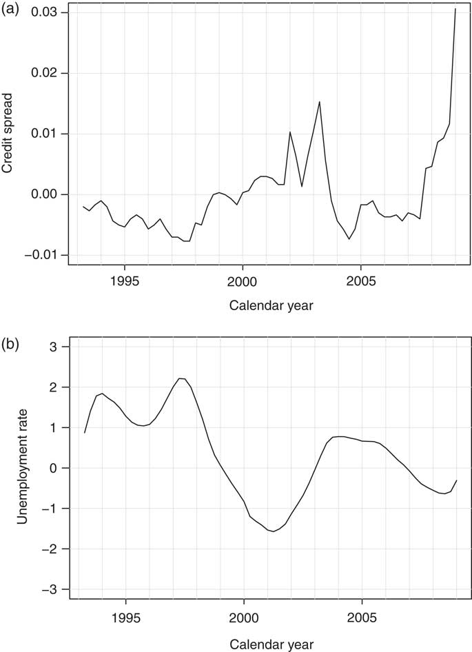
Figure 1 The economic indicator data. The first quarter of 1997 corresponds to calendar period 0. Each series has been normalized by subtracting the average value, so that the normalized series has empirical mean zero. (a) Credit spread data between government and corporate bonds (b) Unemployment rate data.
Running Model 3.5 and assessing the output
To compute the posterior distributions, we used Markov chain Monte Carlo (MCMC) simulation methods. The MCMC methodology provides us with a simulated Markov chain Θ[1],Θ[2],Θ[3],… with
which is an empirical approximation of the posterior distribution ![]() . The computation was implemented in WinBUGS, which is a software program specially designed for such a purpose, to produce 10 000 simulations from the posterior densities of each of the model's parameters. Scollnik (Reference Scollnik2001) gives an overview of MCMC techniques and how they can be implemented in WinBUGS in an actuarial context.
. The computation was implemented in WinBUGS, which is a software program specially designed for such a purpose, to produce 10 000 simulations from the posterior densities of each of the model's parameters. Scollnik (Reference Scollnik2001) gives an overview of MCMC techniques and how they can be implemented in WinBUGS in an actuarial context.
A selection of autocorrelation plots and traceplots for the parameters are shown in Figures 2 and 3, respectively. We used a thinning interval of 50 to reduce the autocorrelations which were observed without any thinning. Boxplots of the posterior parameter distributions are shown in Figure 4. The diagnostic plots in Figure 3 show that convergence has been obtained.

Figure 2 Autocorrelation plots for a selection of the parameters of Model 3.5, using credit spreads as the economic indicator, with a time lag Δ = 5 quarter years and a credibility weight ρ = 0.5. (a) π 1 (b) π 2 (c) γ 3 (d) γ 4 (e) ![]() (f)
(f) ![]() .
.

Figure 3 Traceplots for a selection of the parameters of Model 3.5, using credit spreads as the economic indicator, with a time lag Δ = 5 quarter years and a credibility weight ρ = 0.5. (a) π 1 (b) π 2 (c) γ 3 (d) γ 4 (e) ![]() (f)
(f) ![]() .
.

Figure 4 Boxplots showing the posterior distribution of the parameters of Model 3.5 using credit spreads as the economic indicator, with a time lag Δ = 5 quarter years and a credibility weight ρ = 0.5. (a) Posterior distribution of the parameters π 0,π 1,…,π 47 (b) Posterior distribution of the parameters γ 0,γ 1,…,γ 47 (c) Posterior distribution of the parameters ![]() .
.
Selecting a time lag and economic indicator for Model 3.5
To compare Model 3.5 for different choices of the scalar ρ, time lag Δ and economic indicator series, we used a model selection criterion called the Deviance Information Criterion (DIC). Introduced in Spiegelhalter et al. (Reference Spiegelhalter, Best, Carlin and van der Linde2002), the DIC is a way of comparing Bayesian models by measuring the trade off between the fit of the model to the data and the complexity of the model. Using the DIC as a model selection criterion suggests that we should choose the model with the smallest DIC. However, as it is a relatively ad hoc measure (for criticisms of DIC, see, for example, the discussion in Spiegelhalter et al. Reference Spiegelhalter, Best, Carlin and van der Linde2002), we do not apply this criterion rigorously. Instead, we use it as an approximate guide to the selection of a model. Note that WinBUGS can automatically calculate the DIC.
Choosing credit spreads as the economic indicator, we plot the DIC against the time lag Δ in Figure 5(a). Each line corresponds to a fixed choice of ρ∈{0,0.1,0.2,…, 0.9}. In particular, the horizontal line corresponding to ρ = 0, which corresponds to having no economic indicators in Model 3.5, gives the DIC value for Model 3.1. The DIC values for ρ = 1 are not plotted since they are much higher. For each fixed credibility weight ![]() , the lowest DIC is attained when the time lag is Δ = 5, corresponding to a time lag of 5 quarter years. This suggests that the optimal time lag for the data analyzed is Δ = 5, which is consistent with the optimal time lag obtained by König et al. (Reference König, Weber and Wüthrich2011).
, the lowest DIC is attained when the time lag is Δ = 5, corresponding to a time lag of 5 quarter years. This suggests that the optimal time lag for the data analyzed is Δ = 5, which is consistent with the optimal time lag obtained by König et al. (Reference König, Weber and Wüthrich2011).
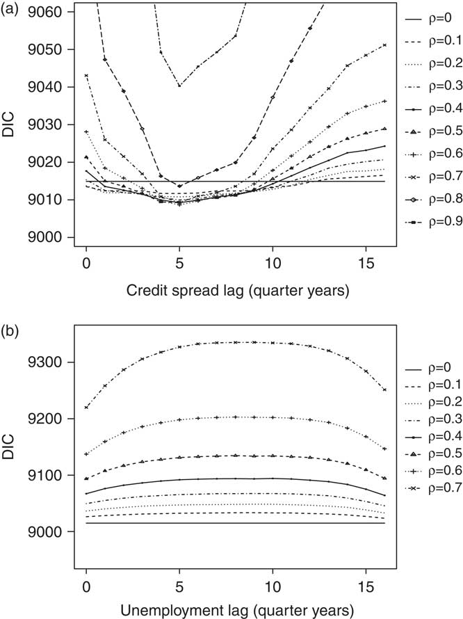
Figure 5 DIC against lags for various fixed values of the credibility weight ρ in Model 3.5. Note the difference in scales. (a) DIC against credit spread lag (b) DIC against unemployment lag.
Fixing the time lag Δ = 5, we see from Figure 5(a) that the lowest DIC value is attained at a credibility weight of ρ = 0.6. However, for ρ∈{0.1,0.2,…, 0.8}, the differences in DIC are not very substantial, being less than 5 units in magnitude. This means that we cannot state with statistical conviction that the model with ρ = 0.6 is the ’’best’’, based on the lowest DIC criterion.
Figure 5(b) shows the results when we choose the unemployment rate as the economic indicator. For each fixed choice of the credibility weight ρ∈{0,0.1,0.2,…, 0.7}, the lowest DIC is obtained when the time lag is Δ = 0, corresponding to no time lag. As the credibility weight ρ is increased, the DIC increases. Again, we do not plot the DIC values for ρ∈{0.8,0.9,1} since they are much higher.
In summary, based on the DIC, using credit spreads as the economic indicator suggests an optimal time lag Δ = 5 and using the unemployment rate as the economic indicator suggests an optimal time lag Δ = 0. In order to improve claims prediction, we prefer an economic indicator which maximizes the time lag and, on this criterion, we prefer to use credit spreads as an economic indicator. Indeed, for the claims data summarized by Table 1, the unemployment rate is not particularly useful as an economic indicator since it has an optimal time lag of zero.
3.4.2 A second model incorporating an economic indicator
Using credit spreads as an economic indicator in Model 3.5, the differences in the DIC at time lag Δ = 5 were not large enough to enable us to choose a particular value of the credibility weight ρ. For this reason, we considered a model which is identical to Model 3.5 except that the credibility weight is modelled as a parameter with a prior distribution, rather than as a constant. The motivation is to find the time lag which allows us to give the most weight to the economic factor ![]() .
.
Model 3.9 Assume Model 3.5 but replace the parameter vector Θ by
and replace assumption (f′) with
(f′′)
in which the credibility weight parameter ρ is independent of all the other parameters and has prior distribution
the random variables ![]() and
and ![]() are independent for all j, k,
are independent for all j, k,
and the scaling factor α is chosen so that the coefficient of variation of ![]() is equal to that of
is equal to that of ![]() for
for ![]() .
.
Remark 3.10 Reflecting the inconclusive results about the optimal value of the credibility weight in Model 3.5, we assume that the prior distribution of the credibility weight parameter is uniformly distributed between 0 and 1. As in Model 3.5, the mean of the error term εk in assumption ![]() is chosen so that
is chosen so that ![]() is a martingale, for
is a martingale, for ![]() .
.
Applying Model 3.9 to the data
We analyzed the same quarterly claims data, applying Model 3.9 with the values of the parameters of the prior distributions as detailed in Remark 3.2 and using credit spreads and the unemployment rate as economic indicators. As before, we use a MCMC method to obtain simulations
from a Markov chain which empirically approximates the posterior distribution ![]() .
.
Running Model 3.9 and assessing the output
A selection of autocorrelation plots and traceplots for the parameters are shown in Figures 6 and 7, respectively. The plots were obtained after using a thinning interval of 50 to reduce the autocorrelations. We observe more autocorrelation and thus a slower rate of convergence than for Model 3.5. Boxplots of the posterior parameter distributions of ![]() and
and ![]() are shown in Figure 8. The effect of the credit spreads are seen clearly in this figure by comparing the mean of
are shown in Figure 8. The effect of the credit spreads are seen clearly in this figure by comparing the mean of ![]() to the mean of λk, for each value of k. By examining Figure 8(a) and Figure 1(a) together, we see that the parameter means in Figure 8(b) decrease when the (normalized) lagged credit spreads are negative and they increase when the lagged credit spreads are positive. The diagnostic plots in Figure 7 show that convergence has been obtained.
to the mean of λk, for each value of k. By examining Figure 8(a) and Figure 1(a) together, we see that the parameter means in Figure 8(b) decrease when the (normalized) lagged credit spreads are negative and they increase when the lagged credit spreads are positive. The diagnostic plots in Figure 7 show that convergence has been obtained.

Figure 6 Autocorrelation plots for a selection of the parameters of Model 3.9, using credit spreads as the economic indicator, with a time lag Δ = 5 quarter years. (a) ρ (b) π 1 (c) γ 3 (d) γ 4 (e) ![]() (f)
(f) ![]() .
.

Figure 7 Traceplots for a selection of the parameters of Model 3.9, using credit spreads as the economic indicator, with a time lag Δ = 5 quarter years. (a) ρ (b) π 1 (c) γ 3 (d) γ 4 (e) ![]() (f)
(f) ![]() .
.

Figure 8 Boxplots showing the posterior distribution of the parameters ![]() and
and ![]() of Model 3.9 using credit spreads as the economic indicator, with a time lag Δ = 5 quarter years. (a) Posterior distribution of the parameters
of Model 3.9 using credit spreads as the economic indicator, with a time lag Δ = 5 quarter years. (a) Posterior distribution of the parameters ![]() (b) Posterior distribution of the parameters λ0,λ1,…,λ47.
(b) Posterior distribution of the parameters λ0,λ1,…,λ47.
Selecting a time lag and economic indicator for Model 3.9
Since the information is given by ![]() (recall (3.5)), the posterior mean of the credibility weight parameter ρ is
(recall (3.5)), the posterior mean of the credibility weight parameter ρ is
In Figure 9(a) the posterior mean ![]() of the credibility weight parameter is plotted against the time lag Δ when we use credit spreads as the economic indicator; this is the solid line. The dashed and dotted lines show a 50% and 95% credible interval about the posterior mean, respectively. The plot shows that the highest posterior mean
of the credibility weight parameter is plotted against the time lag Δ when we use credit spreads as the economic indicator; this is the solid line. The dashed and dotted lines show a 50% and 95% credible interval about the posterior mean, respectively. The plot shows that the highest posterior mean ![]() is attained at time lag Δ = 5. The time lag Δ = 5 is consistent with the results when Model 3.5 is applied to the same data.
is attained at time lag Δ = 5. The time lag Δ = 5 is consistent with the results when Model 3.5 is applied to the same data.

Figure 9 Posterior mean of the credibility weight parameter against time lag, with the dashed lines showing a 50% and 95% credible interval about the mean. (a) Posterior mean of the credibility weight parameters against credit spread lag (b) Posterior mean of the credibility weight parameters against unemployment lag.
Figure 9(b) shows the results when we use the unemployment rate as an economic indicator. For this latter plot, the highest posterior mean ![]() is attained at time lag Δ = 0. This means that not only is the unemployment rate not useful for prediction, but also that the impact of the unemployment rate on the calendar year development factors is very small.
is attained at time lag Δ = 0. This means that not only is the unemployment rate not useful for prediction, but also that the impact of the unemployment rate on the calendar year development factors is very small.
In summary, the analysis of the claims data using Model 3.9 suggests choosing credit spreads as the economic indicator with time lag Δ = 5. This is consistent with the results in Subsection 3.4.1 and König et al. (Reference König, Weber and Wüthrich2011). The unemployment rate is relatively unhelpful, both in its predictive ability and its impact on the claim numbers. This also means that it does not appear worthwhile to extend the model to include both economic indicators.
4 Improving disability prediction
We have considered two Bayesian models which incorporate an economic indicator. Our analysis of these models with the claims data summarized by Table 1 suggests that Models 3.5 and 3.9, with the credit spreads as the economic indicator and a time lag Δ = 5, would improve claims prediction. Here we compare the claims prediction of the latter model against that of Model 3.1, which does not incorporate any economic indicator.
Posterior distribution from MCMC
For Models 3.1 and 3.9 applied to the quarterly claims data, we used MCMC techniques as outlined before to obtain 10000 samples from each of the posterior distributions of the parameters in Θ and ![]() , respectively. From these samples, we can calculate the empirical densities of the parameters. For example, the posterior density
, respectively. From these samples, we can calculate the empirical densities of the parameters. For example, the posterior density ![]() of the credibility weight parameter ρ is plotted in Figure 10. The plot is approximately symmetrical about the mean
of the credibility weight parameter ρ is plotted in Figure 10. The plot is approximately symmetrical about the mean ![]() , with the density tending to zero at values of ρ near zero and 0.5.
, with the density tending to zero at values of ρ near zero and 0.5.

Figure 10 The posterior density plot for the credibility weight parameter ρ given ![]() using credit spreads as the economic indicator with a time lag Δ = 5 in Model 3.9. The solid vertical line shows the posterior mean and the vertical dashed lines show one posterior standard deviation about the posterior mean.
using credit spreads as the economic indicator with a time lag Δ = 5 in Model 3.9. The solid vertical line shows the posterior mean and the vertical dashed lines show one posterior standard deviation about the posterior mean.
The predictive distribution
A considerable advantage of using the Bayesian approach to claims prediction is that we obtain the predictive distribution of every entry ![]() in the lower triangle. With the predictive distribution at hand, one can do various analyses of the total number of future claims. For example, one can calculate any risk measure and thus perform a tail event analysis, which is very important for any solvency consideration.
in the lower triangle. With the predictive distribution at hand, one can do various analyses of the total number of future claims. For example, one can calculate any risk measure and thus perform a tail event analysis, which is very important for any solvency consideration.
Using the relationship
we can sample from the predictive densities ![]() as follows. Let
as follows. Let
denote a sample from the empirical posterior joint density ![]() of the parameters, obtained by the MCMC method. We use this sample to simulate from
of the parameters, obtained by the MCMC method. We use this sample to simulate from ![]() , which by assumption is Poisson distributed with mean
, which by assumption is Poisson distributed with mean ![]() . The result is a sample from
. The result is a sample from ![]() . We do this for each of the 10 000 samples from the posterior joint density
. We do this for each of the 10 000 samples from the posterior joint density ![]() to obtain 10 000 samples from the predictive density
to obtain 10 000 samples from the predictive density ![]() . Repeating this procedure simultaneously for one sample
. Repeating this procedure simultaneously for one sample ![]() and all the cells in the lower triangle, we use the resulting samples to calculate empirically the predictive density
and all the cells in the lower triangle, we use the resulting samples to calculate empirically the predictive density
of the total number of future claims (that is, the sum of the cells in the lower triangle) for Model 3.9. This empirical predictive density of the lower triangle is plotted in Figure 11. The vertical solid line shows the empirical posterior mean

Figure 11 Empirical density function of the predicted total number of claims using credit spreads as the economic indicator with a time lag Δ = 5 in Model 3.9. The solid vertical line shows the posterior mean and the vertical dashed lines show one posterior standard deviation about the posterior mean.
and the vertical dashed lines show one posterior standard deviation about the posterior mean. Notice from Figure 11 that we have positive skewness in the predictive density of the total number of future claims.
Remark 4.1 In (4.1) we can no longer decouple λi +j as in (3.2) since λi +j now depends on the observed credit spread data through the random walk which projects the credit spread data beyond time period I (assumption ![]() ).
).
The main result
As the disability frequency is an important quantity to measure the disability risk of a portfolio, we examine how the prediction of the disability frequency varies between the two models. For Model 3.1, it is given by (3.3) with ![]() . For Model 3.9, the posterior mean predicted disability frequency is given by
. For Model 3.9, the posterior mean predicted disability frequency is given by
For Model 3.9, the posterior mean predicted disability frequency is shown in Figure 12 as a solid line, with the dashed lines indicating a 95% credible interval. The posterior mean predicted disability frequency which results from adopting Model 3.1 is also shown; it is the dashed-dotted line, also with a 95% credible interval indicated by dotted lines. The effect of incorporating the credit spread data is clear; the posterior mean predicted disability frequency is much higher for Model 3.9 than for Model 3.1, especially at the later incurred periods where most of the claims numbers are predicted. For example, for claims which were incurred in period 47 (corresponding to the last quarter of 2008), Model 3.9 gives the posterior mean predicted disability frequency ![]() , whereas Model 3.1 gives
, whereas Model 3.1 gives ![]() . The significantly higher predicted disability frequency for Model 3.9 reflects the increase in credit spreads observed from calendar period 43 onwards (see Figure 1(a)). The increasing credit spreads result in the corresponding calendar period development factors increasing, which means that the predicted number of claims increase too. Indeed, credit spreads were at unusually high levels around calendar periods 47 and 48 (corresponding to the last six months of 2008), due to a breakdown in trust between banks which led to a severe liquidity crisis. If we believe that the crisis was a temporary phenomenon which was highly unusual and had a less severe impact on insured lives than on banks, then we may decide to adjust the credit spread data downwards. However, this is a matter of professional judgment and we have not done any such adjustments in our analysis.
. The significantly higher predicted disability frequency for Model 3.9 reflects the increase in credit spreads observed from calendar period 43 onwards (see Figure 1(a)). The increasing credit spreads result in the corresponding calendar period development factors increasing, which means that the predicted number of claims increase too. Indeed, credit spreads were at unusually high levels around calendar periods 47 and 48 (corresponding to the last six months of 2008), due to a breakdown in trust between banks which led to a severe liquidity crisis. If we believe that the crisis was a temporary phenomenon which was highly unusual and had a less severe impact on insured lives than on banks, then we may decide to adjust the credit spread data downwards. However, this is a matter of professional judgment and we have not done any such adjustments in our analysis.
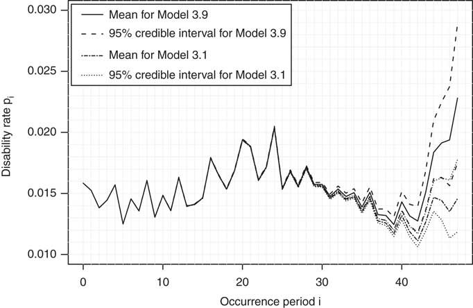
Figure 12 The mean predicted disability rate for Model 3.9, with credit spreads as the economic indicator and time lag Δ = 5 quarter years, and for Model 3.1. The dashed lines show a 95% credible interval about each mean.
Examining the credible intervals in Figure 12, it is clear that they are wider for Model 3.9 than for Model 3.1. This is due to the greater variation in the calendar year development factors of Model 3.9; they are a function not only of the calendar year development factors of Model 3.1 (that is, ![]() ), but also of the credibility weight parameter ρ and the economic indicator data.
), but also of the credibility weight parameter ρ and the economic indicator data.
In summary, the incorporation of credit spread data into the model has resulted in a marked difference in the estimation of the disability risk. Due to the increasing credit spreads which were observed in 2008, the disability risk for claims which were incurred in calendar year 2008 is significantly higher under Model 3.9 than under Model 3.1, which does not incorporate economic data. The results suggest that ignoring economic indicators when predicting claims can result in a significant mis-estimation of the disability risk because these economic indicators correlate with disability rates.
5 Summary
In this paper, we propose a Bayesian model which incorporates an economic indicator. The motivation is to include economic effects which affect the development of the number of disability claims and hence improve the claims prediction. We examined in detail two possible economic indicators: credit spread and the unemployment rate. For the disability claims data we analyzed, there was evidence that credit spreads are useful indicators for claims development, but there was no compelling evidence for incorporating the unemployment rate.
To illustrate the impact of incorporating economic indicators into the Bayesian model, we focused on the disability frequency, which is a measure of the disability risk in a portfolio. Due to the current financial crisis, the mean predicted disability frequency increased sharply when using credit spreads as an economic indicator, as opposed to not using any economic indicator. The results demonstrate how the incorporation of an economic indicator can significantly alter the prediction of the disability risk.
While we found credit spreads to be a reasonable economic indicator, clearly this depended on the data we analyzed. For other datasets, not only may other economic indicators be relevant, but multiple economic indicators could be incorporated into the Bayesian model. However, many economists use credit spreads as a time-lagged indicator of the state of an economy.
It would be interesting to apply a Bayesian model with economic indicators to the amounts of the disability claims, and not only to the number of claims, as well as the effect of economic conditions on the duration of income disability insurance. Unfortunately, we did not have the data to perform these analyses.
Acknowledgments
The authors thank two anonymous referees for comments which improved the paper.


