1 Observation of Power Law Distributions
The observation that the output of natural and social systems follows a heavy-tailed power law distribution has been discussed for some time. Bak et al. (Reference Bak, Tang and Weisenfeld1988) commented that power law relationships have been observed in quasar lights, sunspots, currents through resistors and the flow of rivers. The observation of power law relationships in social systems have also been noted in stock exchange price indices (Bak et al., Reference Bak, Tang and Weisenfeld1988), the structure of the WWW and city sizes (Stumpf & Porter, Reference Stumpf and Porter2012), economic systems (Gabaix, Reference Gabaix2016) and in the commodity market (Fernholz, Reference Fernholz2017). Whilst not specifically discussing power law distributions, earlier papers have observed that financial systems show very heavy tails in their distributions of output. This was found in operational risk events in Evans et al. (Reference Evans, Womersley, Wong and Woodbury2008) and Ganegoda & Evans (Reference Ganegoda and Evans2012) where both papers concluded that banks had very heavy-tailed operational loss distributions. Papers observing the distribution of credit defaults have also observed heavy-tailed distributions (Lucas et al., Reference Lucas, Klaassen, Spreij and Straetmans2001), as have papers observing the distribution of returns in stock markets (de Pinho & dos Santos, Reference de Pinho and dos Santos2013; Gabaix, Reference Gabaix2016).
2 Data
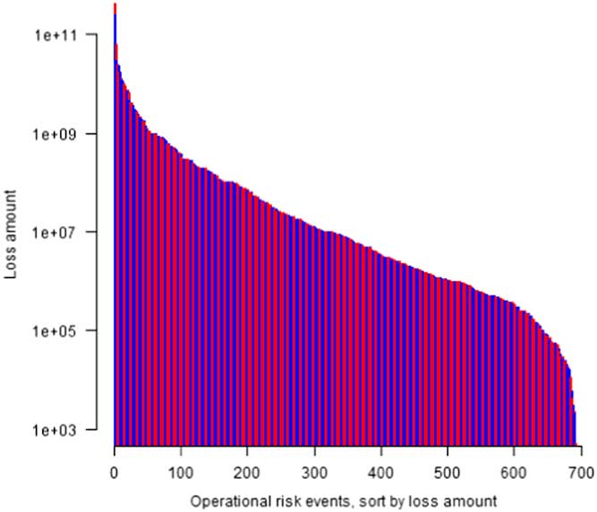
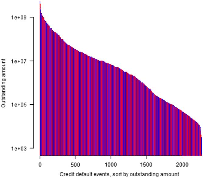
We have examined 380 operational risk eventsFootnote 1 in banks in the United States, 1897 credit defaults in US companiesFootnote 2 and 1762 daily returns of the US stock marketFootnote 3 over the period 2008–2014. Figures 1–3 show for the operational risk losses, credit default losses, and the stock market return the distribution of losses and returns. The X-axis shows each operational risk event, credit default and S&P 500 daily return sorted from largest to smallest, and the Y-axis shows the amount of the operational event loss, credit default loss and return using a logarithmic scale.

Figure 1 Distribution of operational risk losses.

Figure 2 Distribution of credit default losses.

Figure 3 Distribution of stock market return.
3 Analysis of Distributions
Clauset et al. (Reference Clauset, Shalizi and Newman2009) noted that the qualitative observation that had often been used historically to determine if a power law distribution existed is not an adequate basis for concluding the output of a system does follow a power law distribution. Stumpf & Porter (Reference Stumpf and Porter2012) also pointed out that just observation by itself lacks statistical support. We have used the quantitative methodology indicated in Clauset et al. (Reference Clauset, Shalizi and Newman2009) to test for the existence of a power law distribution in the operational risk events, the credit default events and the stock market return. The methodology involves creating a cumulative density function from the data and then testing the goodness of fit with estimated parameters. Table 1 shows the estimated parameters for our data where α is the estimate of the exponent and x min is the lower boundary. Table 2 shows the p-valuesFootnote 4 and goodness of fit values for each of the data sets and indicates that the power law distribution is a good fit for operational risk events, but it is not a good fit for credit defaults and stock market volatility over the period, both of which had heavier tailed distributions than a power law distribution. Table 3 shows the p-values for each data set against a log-normal distribution, and the results indicate the log-normal distribution shows better fit for all three data sets.
Table 1 Estimated parameters for credit risk, market risk and operational risk.

Table 2 Comparison of credit risk, market risk and operational risk distributions to power law distribution.

Table 3 Comparison of data set distributions to log-normal distribution.

Figures 4–6 show a graphical comparison of the distributions for the operational risk losses, credit default losses and stock market return against the distributions predicted by a power law distribution and a log-normal distribution. The observed distributions are shown in black, the best fit power law distribution in red and the best fit log normal distribution in green. The horizontal axis shows the loss amount of operational risk and credit risk losses, and daily return of the S&P 500, and the vertical axis shows the cumulative distribution function (denoted as P(x)).

Figure 4 Comparison of distribution of operational risk losses.

Figure 5 Comparison of distribution of credit default losses.

Figure 6 Comparison of distribution of stock market return.
The issue arising from the results is why is it that a power law distribution is a reasonable estimate of operational risk losses above the truncation point used, but credit defaults and stock market volatility are showing even heavier tails than a power law distribution, and is this difference significant in understanding how these financial systems operated during the global financial crisis (GFC)?
4 Why Did Credit Defaults and Stock Markets Show Heavier-Tailed Distributions Than Operational Risk losses?
The financial system and its subsystems have been shown to be a complex adaptive system (CAS) (Hommes & Wagener, Reference Hommes and Wagener2009; Li et al., 2017 Reference Li, Allan and Evansa ), and a basic feature of a CAS is the existence of power law behaviour and tipping points where the CAS becomes unstable and transitions from a stable environment through to a further stable environment, which may be the same environment as it transitioned from, or a new environment. As observed by Mitleton-Kelly (Reference Mitleton-Kelly2003), where humans are involved in CAS and the system is disrupted well away from the operating norms, the system may reach a critical point and degrade into disorder. This decent into disorder was exactly what was observed in the GFC and it would be reasonable to assume the financial systems would have transitioned from one stable state to another stable state through a period of instability. But this is not appearing in the data, and in fact the contrary situation has occurred with a few much greater losses occurring than predicted from a power law distribution for credit defaults and stock market return and operational risk losses appearing to continue in a stable state. A possible explanation is that the operational risk losses are related to banks which were rescued by governments during the GFC and therefore they continued operating essentially as usual. This implies the global government support for the banks allowed them to continue operations without serious disruption. Corporations were not similarly rescued by governments and they faced liquidity issues as banks declined to roll over loans and consequently they failed to meet loan servicing requirements and defaulted. The stock market would undoubtedly have been influenced by the possibility of corporations failing and greater volatility than expected would have been the consequence as new information flowed through the networks that influence prices in the stock markets. In addition, it is feasible the evolutionary process in the financial systems allows more new combinations of characteristics to occur within the financial institutions, and more quickly than would occur in natural systems which are slower to evolve, and a few of these new combinations in the financial systems then created catastrophic losses. For this to occur it implies that credit assessment techniques in the case of credit defaults and regulatory controls for stability in the case of stock markets did not work, and the new combinations of characteristics went undetected. This makes sense if, as pointed out by Haldane & May (Reference Haldane and May2011), it is assumed institutions and stock market regulators are not considering the characteristics driving the events, but merely looking at the end results and individual system participants. An alternative explanation is offered by Gabaix (Reference Gabaix2016), in that it is possible given the concentration of banks, companies and market capitalisation of listed stocks, and the interconnectivity of the overall financial system (Merton, Reference Merton, Billio, Getmansky, Gray, Lo and Pelizzon2013) that shocks to the larger entities in each of these systems was sufficient to disrupt the whole system, resulting in the catastrophic losses, except for the banking system where the government intervened to stabilise it. Conclusive evidence to support the hypothesis that government intervention precluded operational risks in banks moving to a period of instability is likely to be difficult to find, but the following Table 4 shows that the drivers of US operational risk events as determined by Li et al. (Reference Li, Allan and Evans2017 b) were remarkably stable over the 2008–2014 period for the greatest 10% of operational risk losses (i.e. the heavy tail events). Table 4 shows for the set of drivers of operational risk events used in Li et al. (Reference Li, Allan and Evans2017 b) when a particular driver was involved (X). Had operational risk events been in a transition period then you would not expect such stability.
Table 4 Systemic characteristics for US banks.

It may, however, be easier to determine if credit defaults and stock market volatility exhibited a tipping point which would then result in the heavy-tailed distributions observed.
5 Tipping Point Analysis
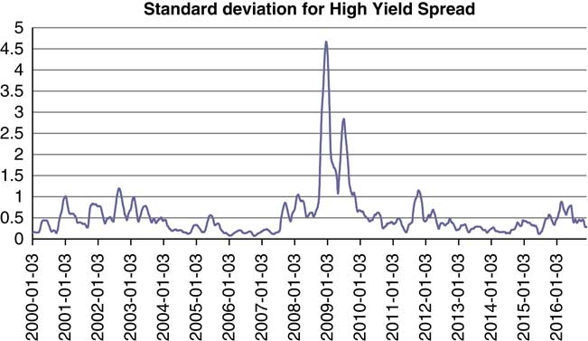
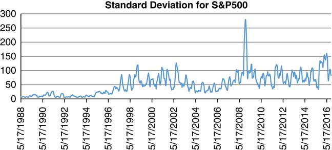
A tipping point is a systems concept, and occurs just before the system changes from states A to B. In this context, “state” refers to the way the system works, i.e., the way the system agents are connected that results in the dynamics of the system. On reaching a tipping point, the system can just move from states A to B and remain there, or it can move back to state A. It may also fall into what is known as an “attractor basin” where it can continually change but always within that basin. The key issue in determining if a tipping point has been reached is whether there has been a change in the dynamics of the system, even for a short period, but this is difficult to analyse in many systems and the alternative of using indicators is more usually adopted. One of the classic indicators used is to detect a “slowing down” of recovery from variability. When a system converges towards a tipping point, it may become more vulnerable to small changes (Holling, Reference Holling1973; Scheffer, Reference Scheffer2001; Dakos et al., Reference Dakos, Scheffer, van Nes, Brovkin, Petoukhov and Held2009) and it will slow down from recovery (Dakos et al., Reference Dakos, Scheffer, van Nes, Brovkin, Petoukhov and Held2009; Scheffer et al., Reference Scheffer, Bascompte, Brock, Brovkin, Capenter, Dakos, Held, Nes, Rietkerk and Sugihara2009), lose resilience and become vulnerable to small shocks, resulting in critical transitions. Takayasu et al. (Reference Takayasu, Watanabe and Takayasu2010) used a relatively simple approach by applying a log-periodic power law model to financial data to detect significant variations, and Lui et al. (Reference Lui, Chen, Aihara and Chen2015) indicated that for systems with significant “normal” volatility, to detect a tipping point, it is better to use a proxy indicator and to consider the second moment of the proxy’s distribution as that dampens down the normal volatility to identify a tipping point. We have combined the methods used by Takayasu et al. (Reference Takayasu, Watanabe and Takayasu2010) and Lui et al. (Reference Lui, Chen, Aihara and Chen2015) to determine if credit defaults and the stock market may have gone through a tipping point in the GFC. Figure 7 shows the standard deviation of the BofA Merrill Lynch US High-Yield Option-Adjusted Spread©, Percent, Daily, Not Seasonally Adjusted on a rolling 90-day basis from 2000 to 2016 as a proxy for credit defaults, and Figure 8 shows the standard deviation of the S&P 500 Composite – Total Return Index on a rolling 90-day basis from 2000 to 2016 as a proxy for market risk.

Figure 7 Standard deviation of high-yield option.

Figure 8 Standard deviation for S&P 500.
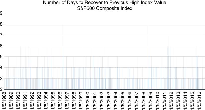
The results in both Figures 7 and 8 show that based on using the standard deviation as an indicator of a tipping point being reached, for both credit defaults and the stock market, a tipping point did occur in 2009 (i.e. well into the GFC), and this may well explain the very heavy-tail distributions then occurring over the 2008–2014 period. We have further considered the other attribute of a tipping point having been reached, namely the slowing down of recovery by the simple method of counting the number of days for the high-yield option spread to return to its previous low after increasing, and the number of days for the S&P 500 index to return to its previous high value after decreasing. The results are shown graphically in Figures 9 and 10, where for ease of analysis we have only shown periods of more than 2 days to recover.

Figure 9 High-yield option spread days to recover to previous low.

Figure 10 S&P500 days to recover to previous high.
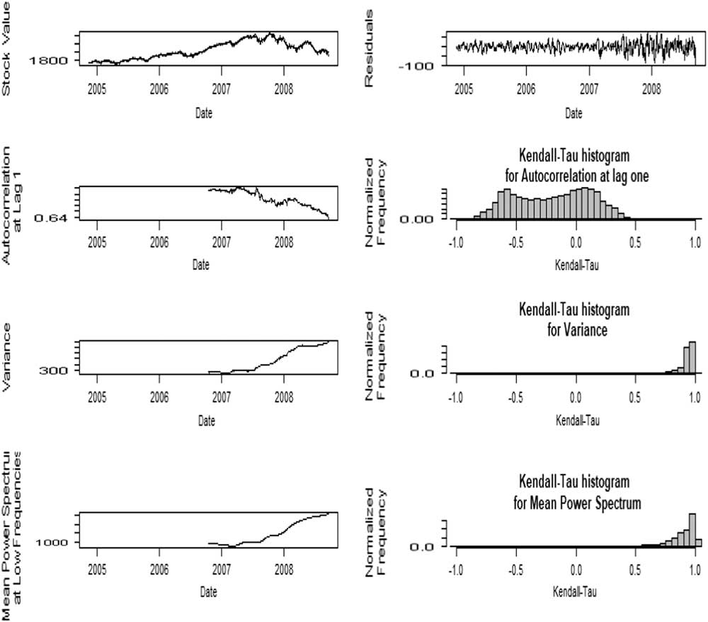
The results in Figures 9 and 10 clearly indicate that around the time of the GFC both the indicators show a significant slowing down of recovery from previous levels. Based on the attributes that for a tipping point to have occurred there should be evidence of a power law distribution breaking down and a slowing down of recovery from variations, it would seem that both credit defaults and the stock market reached a tipping point during the GFC. But, it should be noted there is no universal agreement, and certainly not across academic disciplines as to how to detect a tipping point. Fernholz (Reference Fernholz2017) suggested that volatility in financial systems could be considered as consisting of a volatility component and a reversion component and therefore implied the tipping point concept was not relevant, but we consider this may well just be an alternative description of the tipping point mechanism rather than indicating tipping points do not exist in financial systems. Guttal et al. (Reference Guttal, Raghavendra, Goel and Hoarau2016) and Gatfaoui et al. (Reference Gatfaoui, Nagot and Peretti2017) argued that variance in itself for stock markets was not indicative of having reached a tipping point, and that several stock market crashes that showed significant variance in returns prior to a crash did not show the critical slowing down required for a tipping point having been reached. Figures 11 and 12 shows the results of applying the early warning signals analysis of Guttal et al. (Reference Guttal, Raghavendra, Goel and Hoarau2016) for both credit defaults and the stock market. We use variance, autocorrelation at lag-1 and mean power spectrum as an indicator of the early warning signals, and use Kendall’s τ to present the trend of these indicators. The power spectrum describes the strength of the wave at different frequencies, i.e., at which frequency the signal is strong or weak. An increase in power spectrum low frequency indicates a power increase embedded in variance, hence it can be a signal of critical transition (Kleinen et al., Reference Kleinen, Held and Petschel-Held2003; Guttal et al., Reference Guttal, Raghavendra, Goel and Hoarau2016). The autocorrelation at lag 1, as an important indicator of early warning signal (Dakos et al., Reference Dakos, Scheffer, van Nes, Brovkin, Petoukhov and Held2008; Scheffer et al., 2009), does not present a clear trend prior the GFC, but the variance and mean power spectrum at low frequency increase dramatically before the GFC. Kendall’s τ of autocorrelation at lag-1 shows a distribution from −1 to 1, indicating no clear trend of autocorrelation while Kendall’s τ of variance and mean power spectrum are close to 1, indicating a clear increasing trend.
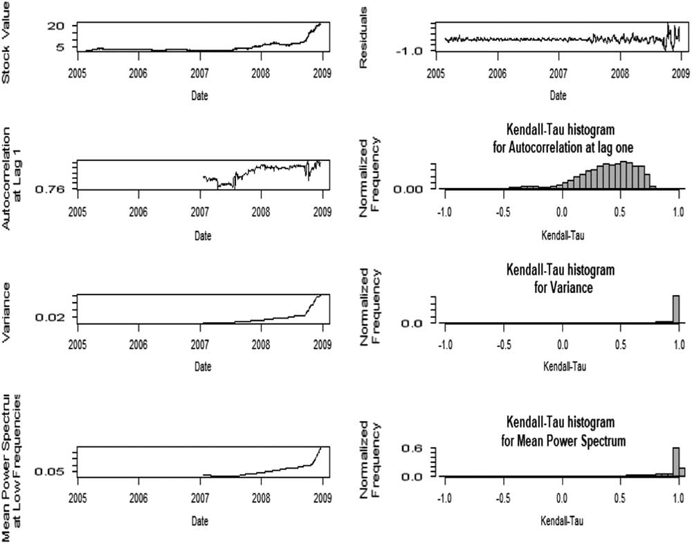
Figure 11 Early warning signals of the global financial crisis based on high-yield option.

Figure 12 Early warning signals of the global financial crisis based on S&P 500.
6 Conclusion
This paper exams three financial sub-systems during the GFC. The quantitative analysis of credit, market and operational risk shows a lack of statistical support for previously observed power law behaviour for credit defaults and stock market returns from 2008 to 2014, and a weak level of support for operational risk losses over that time following a power law distribution. In the case of credit defaults and the stock market, the distributions occurring around the GFC are even heavier tailed than suggested by a power law, indicating some extreme values were reached. These results in themselves suggest a tipping point may have occurred for credit defaults and stock market returns, but not for operational risk losses. Further evidence of credit defaults and stock market returns having reached tipping points but not operational risk losses have been provided using further accepted indicators for credit defaults and stock market returns, and an analysis of the stability of systemic characteristics for operational risk. However, there is not universal agreement on the interpretation of the results, particularly across academic disciplines.
The system based analysis supports the view of Haldane & May (Reference Haldane and May2011) that it is the output of the system that is important, and the quantitative easing practiced by the US Fed does seem to have worked in so far as operational losses were concerned. The analysis then suggests that regulation in the financial market needs to be systems based rather than a reductionist approach to trying to manage individual institutions.
Acknowledgements
The authors would like to acknowledge the valuable comments of an anonymous reviewer that has resulted in an improved paper.