


INTRODUCTION
As the amount and diversity of available data sets rapidly increase, social scientists often harness multiple data sources to answer substantive questions. Indeed, merging data sets, in particular large-scale administrative records, is an essential part of cutting-edge empirical research in many disciplines (e.g., Ansolabehere and Hersh Reference Ansolabehere and Hersh2012; Einav and Levin Reference Einav and Levin2014; Jutte, Roos, and Browne Reference Jutte, Roos and Browne2011). Data merging can be consequential. For example, the American National Election Studies (ANES) and Cooperative Congressional Election Study (CCES) validate self-reported turnout by merging their survey data with a nationwide voter file where only the matched respondents are treated as registered voters. Although Ansolabehere and Hersh (Reference Ansolabehere and Hersh2012) advocate the use of such a validation procedure, Berent, Krosnick, and Lupia (Reference Berent, Krosnick and Lupia2016) argue that the discrepancy between self-reported and validated turnout is due to the failure of the merge procedure rather than social desirability and nonresponse bias.
Merging data sets is straightforward if there exists a unique identifier that unambiguously links records from different data sets. Unfortunately, such a unique identifier is often unavailable. Under these circumstances, some researchers have used a deterministic algorithm to automate the merge process (e.g., Adena et al. Reference Adena, Enikolopov, Petrova, Santarosa and Zhuravskaya2015; Ansolabehere and Hersh Reference Ansolabehere and Hersh2017; Berent, Krosnick, and Lupia Reference Berent, Krosnick and Lupia2016; Bolsen, Ferraro, and Miranda Reference Bolsen, Ferraro and Miranda2014; Cesarini et al. Reference Cesarini, Lindqvist, Ostling and Wallace2016; Figlio and Guryan Reference Figlio and Guryan2014; Giraud-Carrier et al. Reference Giraud-Carrier, Goodlife, Jones and Cueva2015; Hill Reference Hill2017; Meredith and Morse Reference Meredith and Morse2014) whereas others have relied on a proprietary algorithm (e.g., Ansolabehere and Hersh Reference Ansolabehere and Hersh2012; Engbom and Moser Reference Engbom and Moser2017; Figlio and Guryan Reference Figlio and Guryan2014; Hersh Reference Hersh2015; Hill and Huber Reference Hill and Huber2017; Richman, Chattha, and Earnest Reference Richman, Chattha and Earnest2014). However, these methods are not robust to measurement error (e.g., misspelling) and missing data, which are common to social science data. Furthermore, deterministic merge methods cannot quantify the uncertainty of the merging procedure and instead typically rely on arbitrary thresholds to determine the degree of similarity sufficient for matches.Footnote 1 This means that post-merge data analyses fail to account for the uncertainty of the merging procedure, yielding a bias due to measurement error. These methodological challenges are amplified especially when merging large-scale administrative records.
We demonstrate that social scientists should use probabilistic models rather than deterministic methods when merging large data sets. Probabilistic models can quantify the uncertainty inherent in many merge procedures, offering a principled way to calibrate and account for false positives and false negatives. Unfortunately, although there exists a well-known statistics literature on probabilistic record linkage (e.g., Harron, Goldstein, and Dibben Reference Harron, Goldstein and Dibben2015; Herzog, Scheuren, and Winkler Reference Herzog, Scheuren and Winkler2007; Winkler Reference Winkler2006b), the current open-source implementation does not scale to large data sets commonly used in today’s social science research. We address this challenge by developing a fast and scalable implementation of the canonical probabilistic record linkage model originally proposed by Fellegi and Sunter (Reference Fellegi and Sunter1969). Together with parallelization, this algorithm, which we call fastLink, can be used to merge data sets with millions of records in a reasonable amount of time using one’s laptop computer. Additionally, building on the previous methodological literature (e.g., Lahiri and Larsen Reference Lahiri and Larsen2005), we show (1) how to incorporate auxiliary information such as population name frequency and migration rates into the merge procedure and (2) how to conduct post-merge analyses while accounting for the uncertainty about the merge process. We describe these methodological developments in the following section.
We then describe the comprehensive simulation studies to evaluate the robustness of fastLink to several factors including the size of data sets, the proportion of true matches, measurement error, and missing data proportion and mechanisms. A total of 270 simulation settings consistently show that fastLink significantly outperforms the deterministic methods. Although the proposed methodology produces high-quality matches in most situations, the lack of overlap between two data sets often leads to large error rates, suggesting that effective blocking is essential when the expected number of matches is relatively small. Furthermore, fastLink appears to perform at least as well as recently proposed probabilistic approaches (Sadinle Reference Sadinle2017; Steorts Reference Steorts2015). Importantly, our merge method is faster and scales to larger data sets than these state-of-art methods.
Next, we present two empirical applications. First, we revisit Hill and Huber (Reference Hill and Huber2017) who examine the ideological differences between donors and nondonors by merging the CCES data of more than 50,000 survey respondents, with the a campaign contribution database of over five million donor records (Bonica Reference Bonica2013). We find that the matches identified by fastLink are at least as high quality as those identified by the proprietary method, which was used by the original authors. We also improve the original analysis by incorporating the uncertainty of the merge process in the post-merge analysis. We show that although the overall conclusion remains unchanged, the magnitude of the estimated effects is substantially smaller.
As the second application, we merge two nationwide voter files of over 160 million voter records each, representing one of the largest data merges ever conducted in social science research.Footnote 2 By merging voter files over time, scholars can study the causes and consequences of partisan residential segregation (e.g., Tam Cho, Gimpel, and Hui Reference Tam Cho, Gimpel and Hui2013; Mummolo and Nall Reference Mummolo and Nall2016) and political analytics professionals can develop effective microtargeting strategies (e.g., Hersh Reference Hersh2015). We show how to incorporate available within-state and across-state migration rates in the merge process. Given the enormous size of the data sets, we propose a two-step procedure where we first conduct a within-state merge for each state followed by across-state merges for every pair of states. The proposed methodology is able to match about 95% of voters, which is about 30-percentage points greater than the exact matching method. Although it is more difficult to find across-state movers, we are able to find 20 times as many such voters than the existing matching method.
Finally, we give concluding remarks. We provide an open-source R software package fastLink: Fast Probabilistic Record Linkage, which is freely available at the Comprehensive R Archive Network (CRAN; https://CRAN.R-project.org/package=fastLink) for implementing our methodology so that other researchers can effectively merge data sets in their own projects.
THE PROPOSED METHODOLOGY
In this section, we first introduce the canonical model of probabilistic record linkage originally proposed by Fellegi and Sunter (Reference Fellegi and Sunter1969). We describe several improvements we make to this model, including a fast and scalable implementation, the use of auxiliary information to inform parameter estimation, and the incorporation of uncertainty about the merge process in post-merge analyses.
The Setup
Suppose that we wish to merge two data sets,  ${\cal A}$ and
  ${\cal B}$, which have sample sizes of
  ${N_{\cal A}}$ and
  ${N_{\cal B}}$, respectively. We use K variables, which are common to both data sets, to conduct the merge. We consider all possible pair-wise comparisons between these two data sets. For each of these
  ${N_{\cal A}} \times {N_{\cal B}}$ distinct pairs, we define an agreement vector of length K, denoted by γ(i, j), whose kth element γk(i, j) represents the discrete level of within-pair similarity for the kth variable between the ith observation of data set
  ${\cal A}$ and the jth observation of data set
  ${\cal B}$. Specifically, if we have a total of L k similarity levels for the kth variable, then the corresponding element of the agreement vector can be defined as,
 $${\gamma _k}\left( {i,j} \right) = \left\{ {\matrix{ \!\!\!\!\!\!0 & {{\rm{different}}} \cr {\left. {\matrix{ 1 \cr \vdots \cr {{L_k} - 2} \cr} } \right\}} & {{\rm{similar}}} \cr \hskip-9pt{{L_k} - 1} & {{\rm{identical}}} \cr} } \right.$$
The proposed methodology allows for the existence of missing data. We define a missingness vector of length K, denoted by δ(i, j), for each pair (i, j) where its kth element δk(i, j) equals 1 if at least one record in the pair has a missing value in the kth variable and is equal to 0 otherwise.
Table 1 presents an illustrative example of agreement patterns based on two artificial data sets,  ${\cal A}$ and
  ${\cal B}$, each of which has two records. In this example, we consider three possible values of γk(i, j) for first name, last name, and street name, i.e., L k = 3 (different, similar, nearly identical), whereas a binary variable is used for the other fields, i.e., L k = 2 (different, nearly identical). The former set of variables requires a similarity measure and threshold values. We use the Jaro–Winkler string distance (Jaro Reference Jaro1989; Winkler Reference Winkler1990), which is a commonly used measure in the literature (e.g., Cohen, Ravikumar, and Fienberg Reference Cohen, Ravikumar and Fienberg2003; Yancey Reference Yancey2005).Footnote 3 Because the Jaro–Winkler distance is a continuous measure whose values range from 0 (different) to 1 (identical), we discretize it so that γk(i, j) takes an integer value between 0 and L k − 1 as defined in equation (1). Suppose that we use three levels (i.e., different, similar, and nearly identical) based on the threshold values of 0.88 and 0.94 as recommended by Winkler (Reference Winkler1990). Then, when comparing the last names in Table 1, we find that, for example, Smith and Smithson are similar (a Jaro–Winkler distance of 0.88) whereas Smith and Martinez are different (a Jaro–Winkler distance of 0.55).Footnote 4
TABLE 1. An Illustrative Example of Agreement Patterns.

The top panel of the table shows two artificial data sets,  ${\cal A}$ and
  ${\cal B}$, each of which has two records. The bottom panel shows the agreement patterns for all possible pairs of these records. For example, the second line of the agreement patterns compares the first record of the data set
  ${\cal A}$ with the second record of the data set
  ${\cal B}$. These two records have an identical information for first name, date of birth, and house number; similar information for last name and street name; and different information for middle name. A comparison involving at least one missing value is indicated by NA.
The above setup implies a total of  ${N_{\cal A}} \times {N_{\cal B}}$ comparisons for each of K fields. Thus, the number of comparisons grows quickly as the size of data sets increases. One solution is to use blocking and avoid comparisons that should not be made. For example, we may make comparisons within gender group only. While it is appealing because of computational efficiency gains, Winkler (Reference Winkler2005) notes that blocking often involves ad hoc decisions by researchers and faces difficulties when variables have missing values and measurement error. Here, we focus on the data merge within a block and refer interested readers to Christen (Reference Christen2012) and Steorts et al. (Reference Steorts, Ventura, Sadinle, Fienberg and Domingo-Ferrer2014) for comprehensive reviews of blocking techniques.Footnote 5 We also note a related technique, called filtering, which has the potential to overcome the weaknesses of traditional blocking methods by discarding pairs that are unlikely to be matches when fitting a probabilistic model (Murray Reference Murray2016).
The Canonical Model of Probabilistic Record Linkage
The Model and Assumptions
We first describe the most commonly used probabilistic model of record linkage (Fellegi and Sunter Reference Fellegi and Sunter1969). Let a latent mixing variable M ij indicate whether a pair of records (the ith record in the data set  ${\cal A}$ and the jth record in the data set
  ${\cal B}$) represents a match. The model has the following simple finite mixture structure (e.g., Imai and Tingley Reference Imai and Tingley2012; McLaughlan and Peel Reference McLaughlan and Peel2000):
 $$\left. {{\gamma _k}\left( {i,j} \right)} \right\,|\,{M_{ij}} = m\mathop \sim \limits^{{\rm{indep}}{\rm{.}}} \;{\rm{Discrete}}\left( {{{{\boldpi }}_{km}}} \right),$$
 $${M_{ij}}\mathop \sim \limits^{{\rm{i}}{\rm{.i}}{\rm{.d}}{\rm{.}}} \;{\rm{Bernoulli}}\left( \lambda \right),$$
where π km is a vector of length L k, containing the probability of each agreement level for the kth variable given that the pair is a match (m = 1) or a nonmatch (m = 0), and λ represents the probability of a match across all pairwise comparisons. Through π k0, the model allows for the possibility that two records can have identical values for some variables even when they do not represent a match.
This model is based on two key independence assumptions. First, the latent variable M ij is assumed to be independently and identically distributed. Such an assumption is necessarily violated if, for example, each record in the data set  ${\cal A}$ should be matched with no more than one record in the data set
  ${\cal B}$. In theory, this assumption can be relaxed (e.g., Sadinle Reference Sadinle2017) but doing so makes the estimation significantly more complex and reduces its scalability (see Online SI S8). Later in the paper, we discuss how to impose such a constraint without sacrificing computational efficiency. Second, the conditional independence among linkage variables is assumed given the match status. Some studies find that the violation of this assumption leads to unsatisfactory performance (e.g., Belin and Rubin Reference Belin and Rubin1995; Herzog, Scheuren, and Winkler Reference Herzog, Scheuren and Winkler2010; Larsen and Rubin Reference Larsen and Rubin2001; Thibaudeau Reference Thibaudeau1993; Winkler and Yancey Reference Winkler and Yancey2006). In Online SI S4, we show how to relax the conditional independence assumption while keeping our scalable implementation.
In the literature, researchers often treat missing data as disagreements, i.e., γk(i, j) = 0 if δk(i, j) = 1 (e.g., Goldstein and Harron Reference Goldstein and Harron2015; Ong et al. Reference Ong, Mannino, Schilling and Kahn2014; Sariyar, Borg, and Pommerening Reference Sariyar, Borg and Pommerening2012). This procedure is problematic because a true match can contain missing values. Other imputation procedures also exist but none of them has a theoretical justification or appears to perform well in practice.Footnote 6 To address this problem, following Sadinle (Reference Sadinle2014, Reference Sadinle2017), we assume that data are missing at random (MAR) conditional on the latent variable M ij,
 $${\delta _k}\left( {i,j} \right)\, {\perp \!\!\! \perp {\gamma _k}\left( {i,j} \right)\,|\,{M_{ij}},$$
for each  $i = 1,2, \ldots ,{N_{\cal A}}$,
  $j = 1,2, \ldots ,{N_{\cal B}}$, and k = 1, 2, …, K. Under this MAR assumption, we can simply ignore missing data. The observed-data likelihood function of the model defined in equations (2) and (3) is given by,
 $${{\cal L}_{{\rm{obs}}}}\left( {{{\boldlambda }},{{\boldpi }}\,|\,{{\bolddelta }},{{\boldgamma }}} \right) \propto \mathop\prod\limits_{i = 1}^{{N_{\cal A}}} {\mathop\prod\limits_{j = 1}^{{N_{\cal B}}} {\left\{ {\mathop\sum\limits_{m = 0}^1 {{\lambda ^m}{{\left( {1 - \lambda } \right)}^{1 - m}}} \mathop{\scale150%\prod}\limits_{k = 1}^K {{{\left( {\mathop\scale150%\prod\limits_{\ell = 0}^{{L_k} - 1} {\pi _{km\ell }^{1\{ {\gamma _k}(i,j) = \ell \} }} } \right)}^{1 - {\delta _k}\left( {i,j} \right)}}} } \right\}} ,}$$
where  ${\pi _{km\ell }}$ represents the
  $\ell$th element of probability vector π km, i.e.,
  ${\pi _{km\ell }} = \Pr \left( {{\gamma _k}\left( {i,j} \right) = \ell \,|\,{M_{ij}} = m} \right)$. Because the direct maximization of the observed-data log-likelihood function is difficult, we estimate the model parameters using the Expectation-Maximization (EM) algorithm (see Online SI S2).
The Uncertainty of the Merge Process
The advantage of probabilistic models is their ability to quantify the uncertainty inherent in merging. Once the model parameters are estimated, we can compute the match probability for each pair using Bayes rule,Footnote 7
 $$\eqalign{ & {\xi _{ij}} = \Pr \left( {{M_{ij}} = 1\,\,|\,\,\bolddelta \left( {i,j} \right),\gamma \left( {i,j} \right)} \right) \cr & = {{\lambda \prod\limits_{k = 1}^K {{{\left( {\prod\limits_{\ell = 0}^{{L_k} - 1} {\pi _{k1\ell }^{1\{ {\gamma _k}(i,j) = \ell \} }} } \right)}^{1 - {\delta _k}\left( {i,j} \right)}}} } \over {\sum}\limits_{m = 0}^1 {{\lambda ^m}} {{\left( {1 - \lambda } \right)}^{1 - m}}\prod\limits_{k = 1}^K {{{\left( {\prod\limits_{\ell = 0}^{{L_k} - 1} {\pi _{km\ell }^{1\{ {\gamma _k}(i,j) = \ell \} }} } \right)}^{1 - {\delta _k}\left( {i,j} \right)}}} }}. \cr}$$
In the subsection Post-merge Analysis, we show how to incorporate this match probability into post-merge regression analysis to account for the uncertainty of the merge process.
Although in theory a post-merge analysis can use all pairs with nonzero match probabilities, it is often more convenient to determine a threshold S when creating a merged data set. Such an approach is useful especially when the data sets are large. Specifically, we call a pair (i, j) a match if the match probability  $\xi _{ij}$ exceeds S. There is a clear trade-off in the choice of this threshold value. A large value of S will ensure that most of the selected pairs are correct matches but may fail to identify many true matches. In contrast, if we lower S too much, we will select more pairs but many of them may be false matches. Therefore, it is important to quantify the degree of these matching errors in the merging process.
One advantage of probabilistic models over deterministic methods is that we can estimate the false discovery rate (FDR) and the false negative rate (FNR). The FDR represents the proportion of false matches among the selected pairs whose matching probability is greater than or equal to the threshold. We estimate the FDR using our model parameters as follows:
 $${\Pr \left( {{M_{ij}} = 0\,\,|\,\,{\xi _{ij}} \,\,\ge\,\, S} \right)} = {{{{\sum}\limits_{i = 1}^{{N_{\cal A}}} {\sum}\limits_{j = 1}^{{N_{\cal B}}} {{\bf{1}}\left\{ {{\xi _{ij}} \,\,\ge\,\, S} \right\}\left( {1 - {\xi _{ij}}} \right)} } } \over {\sum}\limits_{i = 1}^{{N_{\cal A}}} {\sum}\limits_{j = 1}^{{N_{\cal B}}} {{\bf{1}}\left\{ {{\xi _{ij}} \,\,\ge\,\, S} \right\}} } }}}}},$$
whereas the FNR, which represents the proportion of true matches that are not selected, is estimated as
 $$\Pr \left( {{M_{ij}} = 1\,\,|\,\,{\xi _{ij}} \,\,\lt\,\, S} \right) = {{{\sum}\limits_{i = 1}^{{N_{\cal A}}} {{\sum}\limits_{j = 1}^{{N_{\cal B}}} {{\xi _{ij}}{\bf{1}}\left\{ {{\xi _{ij}} \lt S} \right\}} } } \over {\lambda {N_{\cal A}}{N_{\cal B}}}}.$$
Researchers typically select, at their own discretion, the value of S such that the FDR is sufficiently small. But, we also emphasize the FNR because a strict threshold can lead to many false negatives.Footnote 8 In our simulations and empirical studies, we find that the results are not particularly sensitive to the choice of threshold value, although in other applications, scholars found ex-post adjustments are necessary for obtaining good estimates of error rates (e.g., Belin and Rubin Reference Belin and Rubin1995; Larsen and Rubin Reference Larsen and Rubin2001; Murray Reference Murray2016; Thibaudeau Reference Thibaudeau1993; Winkler Reference Winkler1993; Winkler Reference Winkler2006a).
In the merging process, for a given record in the data set  ${\cal A}$, it is possible to find multiple records in the data set
  ${\cal B}$ that have high match probabilities. In some cases, multiple observations have an identical value of match probability, i.e.,
  $\xi _{ij} = \xi _{ij'}$ with j ≠ j′. Following the literature (e.g., McVeigh and Murray Reference McVeigh and Murray2017; Sadinle Reference Sadinle2017; Tancredi and Liseo Reference Tancredi and Liseo2011), we recommend that researchers analyze all matched observations by weighting them according to the matching probability (see the subsection Post-Merge Analysis). If researchers wish to enforce a constraint that each record in one data set is only matched at most with one record in the other data set, they may follow a procedure described in Online SI S5.
Incorporating Auxiliary Information
Another advantage of the probabilistic model introduced above is that we can incorporate auxiliary information in parameter estimation. This point has not been emphasized enough in the literature. Here, we briefly discuss two adjustments using auxiliary data—first, how to adjust for the fact that some names are more common than others, and second, how to incorporate aggregate information about migration. More details can be found in Online SI S6.
Because some first names are more common than others, they may be more likely to be false matches. To adjust for this possibility without increasing the computational burden, we formalize the conditions under which the ex-post correction originally proposed by Winkler (Reference Winkler2000) is well-suited for this purpose. Briefly, the probability of being a match will be up-weighted or down-weighted given the true frequencies of different first names (obtained, for instance, from Census data) or observed frequencies of each unique first name in the data (see Online SI S6.3.1).
Furthermore, we may know a priori how many matches we should find in two data sets because of the knowledge and data on over-time migration. For instance, the Internal Revenue Service (IRS) publishes detailed information on migration in the United States from tax records (see https://www.irs.gov/uac/soi-tax-stats-migration-data). An estimate of the share of individuals who moved out of a state or who moved in-state can be easily reformulated as a prior on relevant parameters in the Fellegi–Sunter model and incorporated into parameter estimation (see Online SI S6.3.2).
Post-Merge Analysis
Finally, we discuss how to conduct a statistical analysis once merging is complete. One advantage of probabilistic models is that we can directly incorporate the uncertainty inherent to the merging process in the post-merge analysis. This is important because researchers often use the merged variable either as the outcome or as the explanatory variable in the post-merge analysis. For example, when the ANES validates self-reported turnout by merging the survey data with a nationwide voter file, respondents who are unable to be merged are coded as nonregistered voters. Given the uncertainty inherent to the merging process, it is possible that a merging algorithm fails to find some respondents in the voter file even though they are actually registered voters. Similarly, we may incorrectly merge survey respondents with other registered voters. These mismatches, if ignored, can adversely affect the properties of post-match analyses (e.g., Neter, Maynes, and Ramanathan Reference Neter, Maynes and Ramanathan1965; Scheuren and Winkler Reference Scheuren and Winkler1993).
Unfortunately, most of the record linkage literature has focused on the linkage process itself without considering how to conduct subsequent statistical analyses after merging data sets.Footnote 9 Here, we build on a small literature about post-merge regression analysis, the goal of which is to eliminate possible biases due to the linkage process within the Fellegi–Sunter framework (e.g., Hof and Zwinderman Reference Hof and Zwinderman2012; Kim and Chambers Reference Kim and Chambers2012; Lahiri and Larsen Reference Lahiri and Larsen2005; Scheuren and Winkler Reference Scheuren and Winkler1993, Reference Scheuren and Winkler1997). We also clarify the assumptions under which a valid post-merge analysis can be conducted.
The Merged Variable as an Outcome Variable
We first consider the scenario, in which researchers wish to use the variable Z merged from the data set  ${\cal B}$ as a proxy for the outcome variable in a regression analysis. We assume that this regression analysis is applied to all observations of the data set
  ${\cal A}$ and uses a set of explanatory variables X taken from this data set. These explanatory variables may or may not include the variables used for merging. In the ANES application mentioned above, for example, we may be interested in regressing the validated turnout measure merged from the nationwide voter file on a variety of demographic variables measured in the survey.
For each observation i in the data set  ${\cal A}$, we obtain the mean of the merged variable, i.e.,
  ${\zeta _i} = {\mathbb{E}}\left( {Z_i^*\,\,|\,\,\gamma ,{{\bolddelta }}} \right)$ where
  $Z_i^*$ represents the true value of the merged variable. This quantity can be computed as the weighted average of the variable Z merged from the data set
  ${\cal B}$ where the weights are proportional to the match probabilities, i.e.,
  ${\zeta _i} = {{{\sum}\limits_{j = 1}^{{N_{\cal B}}} {{\xi _{ij}}{Z_j}} } / {{\sum}\limits_{j = 1}^{{N_{\cal B}}} {{\xi _{ij}}} }}$. In the ANES application, for example, ζi represents the probability of turnout for survey respondent i in the data set
  ${\cal A}$ and can be computed as the weighted average of turnout among the registered voters in the voter file merged with respondent i. If we use thresholding and one-to-one match assignment so that each record in the data set
  ${\cal A}$ is matched with at most one record in the data set
  ${\cal B}$ (see the subsection The Canonical Model of Probabilistic Record Linkage), then we compute the mean of the merged variable as
  ${\zeta _i} = {\sum}\limits_{j = 1}^{{N_{\cal B}}} {M_{ij}^*{\xi _{ij}}{Z_j}}$ where
  $M_{ij}^*$ is a binary variable indicating whether record i in the data set
  ${\cal A}$ is matched with record j in the data set
  ${\cal B}$ subject to the constraint
  ${\sum}\limits_{j = 1}^{{N_{\cal B}}} {M_{ij}^*} \le 1$.
Under this setting, we assume that the true value of the outcome variable is independent of the explanatory variables in the regression conditional on the information used for merging, i.e.,
 $$Z_i^* \perp \!\!\! \perp {{\bf{X}}_i}\,\,|\,\,\left( {\bolddelta ,\gamma } \right),$$
for each  $i = 1,2, \ldots ,{N_{\cal A}}$. The assumption implies that the merging process is based on all relevant information. Specifically, within an agreement pattern, the true value of the merged variable
  $Z_i^{\rm{*}}$ is not correlated with the explanatory variables Xi. Under this assumption, the law of iterated expectation implies that regressing ζi on Xi gives the results equivalent to the ones based on the regression of
  $Z_i^*$ on Xi in expectation.
 $${\mathbb{{E}}}\left( {Z_i^*\,\,|\,\,{{\bf{X}}_i}} \right) = {\mathbb{E}}\left\{ {{\mathbb{E}}\left( {Z_i^*\,\,|\,\,{{\boldgamma }},{{\bolddelta }},{{\bf{X}}_i}} \right)\,\,|\,\,{{\bf{X}}_i}} \right\} = {\mathbb{E}}\left( {{\zeta _i}\,\,|\,\,{{\bf{X}}_i}} \right).$$
The conditional independence assumption may be violated if, for example, within the same agreement pattern, a variable correlated with explanatory variables is associated with merging error. Without this assumption, however, only the bounds can be identified (Cross and Manski Reference Cross and Manski2002). Thus, alternative assumptions such as parametric assumptions and exclusion restrictions are needed to achieve identification (see Ridder and Moffitt Reference Ridder and Moffitt2007, for a review).
The Merged Variable as an Explanatory Variable
The second scenario we consider is the case where we use the merged variable as an explanatory variable. Suppose that we are interested in fitting the following linear regression model:
 $${Y_i} = \alpha + \beta Z_i^* + {\eta ^ \top }{{\bf{X}}_i} + {\varepsilon _i},$$
where Y i is a scalar outcome variable and the strict exogeneity is assumed, i.e.,  ${\mathbb{E}}\left( {{\varepsilon _i}\,\,|\,\,{Z^*},{\bf{X}}} \right) = 0$ for all i. We follow the analysis strategy first proposed by Lahiri and Larsen (Reference Lahiri and Larsen2005) but clarify the assumptions required for their approach to be valid (see also Hof and Zwinderman Reference Hof and Zwinderman2012). Specifically, we maintain the assumption of no omitted variable for merging given in equation (7). Additionally, we assume that the merging variables are independent of the outcome variable conditional on the explanatory variables Z* and X, i.e.,
 $${Y_i} \perp \!\!\!\perp \left( {{{\boldgamma }},{{\bolddelta }}} \right)\,\,|\,\,{{\bf{Z}}^*},{\bf{X}}.$$
Under these two assumptions, we can consistently estimate the coefficients by regressing Y i on ζi and Xi,
 $$\eqalign{ & {\mathbb{E}}\left( {{Y_i}\,\,|\,\,{{\boldgamma }},{{\bolddelta }},{{\bf{X}}_i}} \right) = \alpha + \beta {\mathbb{E}}\left( {Z_i^*\,\,|\,\,{{\boldgamma }},{{\bolddelta }},{{\bf{X}}_i}} \right) + {\eta ^ \top }{{\bf{X}}_i} + {\mathbb{E}}\left( {{\varepsilon _i}\,\,|\,\,{{\boldgamma }},{{\bolddelta }},{{\bf{X}}_i}} \right) \hskip-8.5pt\qquad\qquad\quad\qquad= \alpha + \beta {\zeta _i} + {\eta ^ \top }{{\bf{X}}_i}, \cr}$$
where the second equality follows from the assumptions and the law of iterated expectation.
We generalize this strategy to the maximum likelihood (ML) estimation, which, to the best of our knowledge, has not been considered in the literature (but see Kim and Chambers (Reference Kim and Chambers2012) for an estimating equations approach),
 $${Y_i}\,\,|\,\,Z_i^*,{{\bf{X}}_i}}\mathop \sim \limits^{{\rm{indep}}{\rm{.}}} {P_\theta }\left( {{Y_i}\,\,|\,\,Z_i^*,{{\bf{X}}_i}} \right),$$
where θ is a vector of model parameters. To estimate the parameters of this model, we maximize the following weighted log-likelihood function:
 $${{\hat{\boldtheta }}} = \mathop {{\rm{argmax}}}\limits_\theta \mathop{\sum}\limits_{i = 1}^{{N_{\cal A}}} {\mathop{\sum}\limits_{j = 1}^{{N_{\cal B}}} {\xi _{ij}^*\log {P_\theta }\left( {{Y_i}\,\,|\,\,Z_i^* = {Z_j},{{\bf{X}}_i}} \right)} } ,$$
where  $\xi _{ij}^* = {{{\xi _{ij}}} / {{\sum}\limits_{j\prime = 1}^{{N_{\cal B}}} {{\xi _{ij\prime }}} }}$. Online SI S7 shows that under the two assumptions described earlier and mild regularity conditions, the weighted ML estimator given in equation (13) is consistent and asymptotically normal. Note that because we are considering large data sets, we ignore the uncertainty about
  $\xi _{ij}^*$.
SIMULATION STUDIES
We conduct a comprehensive set of simulation studies to evaluate the statistical accuracy and computational efficiency of our probabilistic modeling approach and compare them with those of deterministic methods. Specifically, we assess the ability of the proposed methodology to control estimation error, false positives and false negatives, and its robustness to missing values and noise in the linkage fields, as well as the degree of overlap between two data sets to be merged. We do so by systematically varying the amount and structure of missing data and measurement error.
The Setup
To make our simulation studies realistic, we use a data set taken from the 2006 California voter file. Because merging voter files is often done by blocking on gender, we subset the data set to extract the information about female voters only, reducing the number of observation to approximately 17 million voters to 8.3 million observations. To create a base data set for simulations, we further subset the data set by removing all observations that have at least one missing value in the following variables: first name, middle initial, last name, date of birth, registration date, address, zip code, and turnout in the 2004 Presidential election. After listwise deletion, we obtain the final data set of 341,160 voters, from which we generate two data sets of various characteristics to be merged. From this data set, we independently and randomly select two subsamples to be merged under a variety of scenarios.
We design our simulation studies by varying the values of the five parameters as summarized below. Online SI S9.1 describes in detail the precise setups of these simulations.
1. Degree of overlap: Proportion of records in the smaller data set that are also in the larger data set. We consider three scenarios—20% (small), 50% (medium), and 80% (large).
2. Size balance: Balance of sample sizes between the two data sets to be merged. We consider three ratios—1:1 (equally sized), 1:10 (imbalanced), and 1:100 (lopsided).
3. Missing data: We consider five different mechanisms, missing completely at random (MCAR), MAR, and not missing at random (NMAR). For MAR and NMAR, we consider independent and dependent missingness patterns across linkage fields.
4. Amount of missing data: Proportion of missing values in each linkage variable other than year of birth. We consider three scenarios—5% (small), 10% (medium), and 15% (large).
5. Measurement error: Proportion of records (6%) for which the first name, last name, and street name contain a classical measurement error.
Together, we conduct a total of 135 (=33 × 5) simulation studies where missing data are of main concern. We also conduct another set of 135 simulations with various types of nonclassical measurement errors, while keeping the amount of missing values fixed (see Online SI S9.2).
Results
Figure 1 compares the performance of fastLink (blue solid bars) to the two deterministic methods often used by social scientists. The first is the merging method based on exact matches (red shaded bars), whereas the second is the recently proposed partial match algorithm (ADGN; light green solid bars) that considers two records as a match if at least three fields of their address, date of birth, gender, and name are identical (Ansolabehere and Hersh Reference Ansolabehere and Hersh2017). The top panel of Figure 1 presents the FNR whereas the bottom panel presents the absolute error for estimating the 2004 turnout rate. We merge two data sets of equal size (100,000 records each) after introducing the classical measurement error and the medium amount of missing data as explained above. For fastLink, only pairs with a match probability ≥0.85 are considered to be matches, but the results remain qualitatively similar if we change the threshold to 0.75 or 0.95.

FIGURE 1. Accuracy of Data Merge
The top and bottom panels present the false negative rate (FNR) and the absolute estimation error (for estimating the turnout rate), respectively, when merging datasets of 100,000 records each across with different levels of overlap (measured as a percentage of a data set). Three missing data mechanisms are studied with the missing data proportion of 10% for each linkage field other than year of birth: missing completely at random (MCAR), missing at random (MAR), and missing not at random (MNAR). Classical measurement error is introduced to several linkage fields. The proposed probabilistic methodology (fastLink; blue solid bars) significantly outperforms the two deterministic algorithms, i.e., exact match (red shaded bars) and partial match (ADGN; light green solid bars), across simulation settings.
We find that fastLink significantly outperforms the two deterministic methods.Footnote 10 Although all three methods are designed to control the FDR, only fastLink is able to keep the FNR low (less than five percentage in all cases considered here). The deterministic algorithms are not robust to missing data and measurement error, yielding a FNR of much greater magnitude. Additionally, we observe that the deterministic methods yield a substantially greater estimation bias than fastLink unless the data are MCAR. Under the other two missing data mechanisms, the magnitude of the bias is substantially greater than that of fastLink. Although fastLink has an absolute estimation error of less than 1.5 percentage points even under MNAR, the other two methods have an absolute estimation error of more than 7.5 percentage points under both MAR and MNAR. Finally, the performance of fastLink worsens as the size of overlap reduces and the missing data mechanism becomes less random.
We next evaluate the accuracy of FDR and FNR estimates in the top and bottom panels, respectively. Because the deterministic methods do not give such error estimates, we compare the performance of the proposed methodology (indicated by blue solid circles) with that of the same probabilistic modeling approach, which treats missing values as disagreements following a common practice in the literature (indicated by solid triangles). Figure 2 presents the results of merging two data sets of equal size where the medium amount of data are assumed to be MAR and some noise are added as described earlier. In the top panel of the figure, we find that the true FDR is low and its estimate is accurate unless the degree of overlap is small. With a small degree of overlap, both methods significantly underestimate the FDR. A similar finding is obtained for the FNR in the bottom panel of the figure where estimated FNR is biased upward.

FIGURE 2. Accuracy of FDR and FNR Estimates
The top panel compares the estimated FDR (x-axis) with its true value (y-axis) whereas the bottom panel compares the estimated FNR against its true value. We consider the medium amount of missing data generated under MAR as a missingness mechanism and add measurement error to some linkage fields. The blue solid circles represent the estimates based on fastLink whereas the black solid triangles represent the estimates obtained by treating missing data as disagreements. The FDR and FNR estimates are accurate when the overlap is high. Additionally, fastLink gives lower FDR and FNR than the same algorithm that treats missing values as a disagreement. Note that in cases where the overlap is small (20%), blocking improves the precision of our estimates.
One way to address the problem of having small overlap would be to use blocking based on a set of fully observed covariates. For example, in our simulations, because the year of birth is observed for each record in both data sets, we block the data by making comparisons only across individuals within a window of ±1 year around each birth year.Footnote 11 Then, we apply fastLink to each block separately. As shown in the right most column of Figure 2, blocking significantly improves the estimation accuracy for the FDR and FNR estimates as well as their true values although the bias is not eliminated. The reason for this improvement is that traditional blocking increases the degree of overlap. For example, in this simulation setting for each of the 94 blocks under consideration, the ratio of true matches to all possible pairs is at least 8 × 10⁻⁵, which is more than 15 times as large as the corresponding ratio for no blocking and is comparable to the case of overlap of 50%.
We present the results of the remaining simulation studies in the Online Simulation Appendix. Two major patterns discussed above are also found under these other simulation scenarios. First, regardless of the missing data mechanisms and the amount of missing observations, fastLink controls FDR, FNR, and estimation error well. Second, a greater degree of overlap between data sets leads to better merging results in terms of FDR and FNR as well as the accuracy of their estimates. Blocking can ameliorate these problems caused by small overlap to some extent. These empirical patterns are consistently found across simulations even when two data sets have unequal sizes.
Computational Efficiency
We compare the computational performance of fastLink with that of the RecordLinkage package in R (Sariyar and Borg Reference Sariyar and Borg2016) and the Record Linkage package in Python (de Bruin Reference de Bruin2017) in terms of running time. The latter two are the only other open source packages in R and Python that implement a probabilistic model of record linkage under the Fellegi–Sunter framework. To mimic a standard computing environment of applied researchers, all the calculations are performed in a Macintosh laptop computer with a 2.8 GHz Intel Core i7 processor and 8 GB of RAM.
Although fastLink takes advantage of a multicore machine via the OpenMP-based parallelization (the other two packages do not have a parallelization feature), we perform the comparison on a single-core computing environment so that we can assess the computational efficiency of our algorithm itself. Additionally, we include runtime results where we parallelize computation across eight cores. For all implementations, we set the convergence threshold to 1 × 10⁻⁵.Footnote 12
We consider the setup in which we merge two data sets of equal size with 50% overlap, 10% missing proportion under MCAR, and no measurement error. Our linkage variables are first name, middle initial, last name, house number, street name, and year of birth. We vary the size of each data set from 1,000 records to 300,000 observations. As in the earlier simulations, each data set is based on the sample of 341,160 female registered voters in California, for whom we have complete information in each linkage field. To build the agreement patterns, we use the Jaro–Winkler string distance with a cutoff of 0.94 for first name, last name, and street name. For the remaining fields, we only consider exact matches as agreements.
Figure 3 presents the results of this running time comparison. We find that although all three packages take a similar amount of time for data sets of 1,000 records, the running time increases exponentially for the other packages in contrast to fastLink (black solid triangles connected by a dashed line, single core; blue solid circles connected by a solid line, eight cores), which exhibits a near linear increase. When matching data sets of 150,000 records each, fastLink takes less than six hours to merge using a single core (under three hours when parallelized across eight cores). In contrast, it takes more than 24 hours for Record Linkage (Python; solid purple squares connected by a dotted line), to merge two data sets of only 20,000 observations each. The performance is not as bad for Record Linkage (R; red crosses connected by a dashed line), but it still takes over six hours to merge data sets of 40,000 records each. Moreover, an approximation based on an exponential regression model suggests that Record Linkage (R) would take around 22 hours to merge two data sets of 50,000 records each, while Record Linkage (Python) would take about 900 days to accomplish the same merge. In Online SI S3.1, we further decompose the runtime comparison to provide more detail on the sources of our computational improvements. We detail the choices we make in the computational implementation that yields these substantial efficiency gains in Appendix A.

FIGURE 3. Running Time Comparison
The plot presents the results of merging datasets of equal size using different implementations of the Fellegi-Sunter model. The datasets were constructed from a sample of female registered voters in California. The amount of overlap between datasets is 50%, and, for each dataset, there are 10% missing observations in each linkage variable: first name, middle initial, last name, house number, street name, and year of birth. The missing data mechanism is Missing Completely at Random (MCAR). The computation is performed on a Macintosh laptop computer with a 2.8 GHz Intel Core i7 processor and 8 GB of RAM. The proposed implementation fastLink (single-core runtime as black solid triangles connected by a dashed line, and parallelized over eight cores as blue solid dots connected by a solid line) is significantly faster than the other open-source packages.
EMPIRICAL APPLICATIONS
In this section, we present two empirical applications of the proposed methodology. First, we merge election survey data (about 55,000 observations) with political contribution data (about five million observations). The major challenge of this merge is the fact that the expected number of matches between the two data sets is small. Therefore, we utilize blocking and conduct the data merge within each block. The second application is to merge two nationwide voter files, each of which has more than 160 million records. This may, therefore, represent the largest data merge ever conducted in the social sciences. We show how to use auxiliary information about within-state and across-state migration rates to inform the match.
Merging Election Survey Data with Political Contribution Data
Hill and Huber (Reference Hill and Huber2017) study differences between donors and nondonors by merging the 2012 CCES survey with the Database on Ideology, Money in Politics, and Elections [DIME, Bonica (Reference Bonica2013)]. The 2012 CCES is based on a nationally representative sample of 54,535 individuals recruited from the voting-age population in the United States. The DIME data, on the other hand, provide the information about individual donations to political campaigns. For the 2010 and 2012 elections, the DIME contains over five million donors.
The original authors asked YouGov, the company which conducted the survey, to merge the two data sets using a proprietary algorithm. This yielded a total of 4,432 CCES respondents matched to a donor in the DIME data. After the merge, Hill and Huber (Reference Hill and Huber2017) treat each matched CCES respondent as a donor and conduct various analyses by comparing these matched respondents with those who are not matched with a donor in the DIME data and hence are treated as nondonors. Below, we apply the proposed methodology to merge these two data sets and conduct a post-merge analysis by incorporating the uncertainty about the merge process.
Merge Procedure
We use the name, address, and gender information to merge the two data sets. To protect the anonymity of CCES respondents, YouGov used fastLink to merge the data sets on our behalf. Moreover, because of contractual obligations, the merge was conducted only for 51,184 YouGov panelists, which is a subset of the 2012 CCES respondents. We block based on gender and state of residence, resulting in 102 blocks (50 states plus Washington DC × two gender categories). The size of each block ranges from 175,861 (CCES = 49, DIME = 3,589) to 790,372,071 pairs (CCES = 2,367, DIME = 333,913) with the median value of 14,048,151 pairs (CCES = 377, DIME = 37,263). Within each block, we merge the data sets using the first name, middle initial, last name, house number, street name, and postal code. As done in the simulations, we use three levels of agreement for the string-valued variables based on the Jaro–Winkler distance with 0.85 and 0.92 as the thresholds. For the remaining variables (i.e., middle initial, house number, and postal code), we utilize a binary comparison indicating whether they have an identical value.
To construct our set of matched pairs between CCES and DIME, first, we use the one-to-one matching assignment algorithm described in Online SI S5 and find the best match in the DIME data for each CCES respondent. Then, we declare as a match any pair whose matching probability is above a certain threshold. We use three thresholds, i.e., 0.75, 0.85, and 0.95, and examine the sensitivity of the empirical results to the choice of threshold value.Footnote 13 Finally, in the original study of Hill and Huber (Reference Hill and Huber2017), noise is added to the amount of contribution to protect the anonymity of matched CCES respondents. However, we signed a nondisclosure agreement with YouGov for our analysis so that we can make a precise comparison between the proposed methodology and the proprietary merge method used by YouGov.
Merge Results
Table 2 presents the merge results. We begin by assessing the match rates, which represent the proportion of CCES respondents who are matched with donors in the DIME data. Although the match rates are similar between the two methods, fastLink appears to find slightly more (less) matches for male (female) respondents than the proprietary method regardless of the threshold used. However, this does not mean that both methods find identical matches. In fact, out of 4,797 matches identified by fastLink (using the threshold of 0.85), the proprietary method does not identify 861 or 18% of them as matches.
TABLE 2. The Results of Merging the 2012 Cooperative Congressional Election Study (CCES) with the 2010 and 2012 Database on Ideology, Money in Politics, and Elections (DIME) Data

The table presents the merging results for both fastLink and the proprietary method used by YouGov. The results of fastLink are presented for one-to-one match with three different thresholds (i.e., 0.75, 0.85, 0.95) for the matching probability to declare a pair of observations as a successful match. The number of matches, the amount of overlap, and the overall match rates are similar between the two methods. The table also presents information on the estimated false discovery and false negative rates (FDR and FNR, respectively) obtained using fastLink. These statistics are not available for the proprietary method.
As discussed in the subsection The Canonical Model of Probabilistic Record Linkage, one important advantage of the probabilistic modeling approach is that we can estimate the FDR and FNR, which are shown in the table. Such error rates are not available for the proprietary method. As expected, the overall estimated FDR is controlled to less than 1.5% for both male and female respondents. The estimated FNR, on the other hand, is large, illustrating the difficulty of finding some donors. In particular, we find that female donors are much more difficult to find than male donors.
Specifically, there are 12,803 CCES respondents who said they made a campaign contribution during the last 12 months before the 2012 election. Among them, 5,206 respondents claimed to have donated at least 200 dollars. Interestingly, both fastLink and the proprietary method matched an essentially identical number of self-reported donors with a contribution of over 200 dollars (2,431 and 2,434 or approximately 47%, respectively), whereas among the self-reported small donors both methods can only match approximately 16% of them.
Next, we examine the quality of matches for the two methods (see also Online SI S13). We begin by comparing the self-reported donation amount of matched CCES respondents with their actual donation amount recorded in the DIME data. Although only donations greater than 200 dollars are recorded at the federal level, the DIME data include some donations of smaller amounts, if not all, at the state level. Thus, although we do not expect a perfect correlation between self-reported and actual donation amount, under the assumption that donors do not systematically under or over report the amount of campaign contributions, a high correlation between the two measures implies a more accurate merging process.
The upper panel of Figure 4 presents the results where for fastLink, we use one-to-one match with the threshold of 0.85.Footnote 14 We find that for the respondents who are matched by both methods, the correlation between the self-reported and matched donation amounts is reasonably high (0.73). In the case of respondents who are matched by fastLink only, we observe that the correlation is low (0.57) but is greater than the correlation for those matches identified by the proprietary method alone (0.42). We also examine the distribution of match probabilities for these three groups of matches. The bottom panel of the figure presents the results, which are consistent with the patterns of correlation identified in the top panel. That is, those matches identified by the two methods have the highest match probability whereas most of the matches identified only by the proprietary method have extremely low match probabilities. In Online SI S13, we also examine the quality of the agreement patterns separately for the matches identified by both methods, fastLink only, and the proprietary method only. Overall, our results indicate that fastLink produces matches whose quality is often better than that based on the proprietary method.
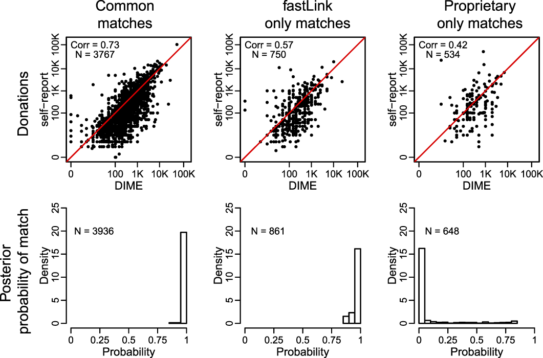
FIGURE 4. Comparison of fastLink and the Proprietary Method
The top panel compares the self-reported donations (y-axis) by matched CCES respondents with their donation amount recorded in the DIME data (x-axis) for the three different groups of observations: those declared as matches by both fastLink and the proprietary method (left), those identified by fastLink only (middle), and those matched by the proprietary method only (right). The bottom panel presents histograms for the match probability for each group. For fastLink, we use one-to-one match with the threshold of 0.85.
Post-Merge Analysis
An important advantage of the probabilistic modeling approach is its ability to account for the uncertainty of the merge process in post-merge analyses. We illustrate this feature by revisiting the post-merge analysis of Hill and Huber (Reference Hill and Huber2017). The original authors are interested in the comparison of donors (defined as those who are matched with records in the DIME data) and nondonors (defined as those who are not matched) among CCES respondents. Using the matches identified by a proprietary method, Hill and Huber (Reference Hill and Huber2017) regress policy ideology on the matching indicator variable, which is interpreted as a donation indicator variable, the turnout indicator variables for the 2012 general election and 2012 congressional primary elections, as well as several demographic variables. Policy ideology, which ranges from −1 (most liberal) to 1 (most conservative), is constructed by applying a factor analysis to a series of questions on various issues.Footnote 15 The demographic control variables include income, education, gender, household union membership, race, age in decades, and importance of religion. The same model is fitted separately for Democrats and Republicans.
To account for the uncertainty of the merge process, as explained in the subsection Post-Merge Analysis, we fit the same linear regression except that we use the mean of the match indicator variable as the main explanatory variable rather than the match indicator variable. Table 3 presents the estimated coefficients of the aforementioned linear regression models with the corresponding heteroskedasticity-robust standard errors in parentheses. Generally, the results of our improved analysis agree with those of the original analysis, showing that donors tend to be more ideologically extreme than nondonors.
TABLE 3. Predicting Policy Ideology Using Contributor Status

The estimated coefficients from the linear regression of policy ideology score on the contributor indicator variable and a set of demographic controls. Along with the original analysis, the table presents the results of the improved analysis based on fastLink, which accounts for the uncertainty of the merge process. *** p < 0.001, ** p < 0.01, * p < 0.05. Robust standard errors in parentheses.
Although the overall conclusion is similar, the estimated coefficients are smaller in magnitude when accounting for the uncertainty of merge process. In particular, according to fastLink, for Republican respondents, the estimated coefficient of being a donor represents only 12% of the standard deviation of their ideological positions (instead of 21% given by the proprietary method). Indeed, the difference in the estimated coefficients between fastLink and the proprietary method is statistically significant for both Republicans (0.035, s.e. = 0.014), and Democrats (−0.015, s.e. = 0.007). Moreover, although the original analysis find that the partisan mean ideological difference for donors (1.108, s.e. = 0.018) is 31 percentage larger than that for nondonors (0.848, s.e. = 0.001), the results based on fastLink shows that this difference is only 25 percentage larger for donors (1.058, s.e. = 0.018). Thus, although the proprietary method suggests that the partisan gap for donors is similar to the partisan gap for those with a college degree or higher (1.100, s.e. = 0.036), fastLink shows that it is closer to the partisan gap for those with just some college education but without a degree (1.036, s.e. = 0.035).
Merging Two Nationwide Voter Files Over Time
Our second application is what might be the largest data merging exercise ever conducted in social sciences. Specifically, we merge the 2014 nationwide voter file to the 2015 nationwide voter file, each of which has over 160 million records. The data sets are provided by L2, Inc., a leading national non-partisan firm and the oldest organization in the United States that supplies voter data and related technology to candidates, political parties, pollsters, and consultants for use in campaigns. In addition to the sheer size of the data sets, merging these nationwide voter files is methodologically challenging because some voters change their residence over time, making addresses uninformative for matching these voters.
Merge Procedure
When merging data sets of this scale, we must drastically reduce the number of comparisons. In fact, if we examine all possible pairwise comparisons between the two voter files, the total number of such pairs exceeds 2.5 × 10¹⁶. It is also important to incorporate auxiliary information about movers because the address variable is noninformative when matching these voters. We use the IRS Statistics of Income (SOI) to calibrate match rates for within-state and across-state movers. Details on incorporating migration rates into parameter estimation can be found in the subsection Incorporating Auxiliary Information and Online SI S6.2. The IRS SOI data are definitive source of migration data in the United States that tracks individual residences year-to-year across all states through their tax returns.
We develop the following two-step procedure that utilizes random sampling and blocking of voter records to reduce the computational burden of the merge (see Online SI S3.2 and S6.2). Our merge is based on first name, middle initial, last name, house number, street name, date/year/month of birth, date/year/month of registration, and gender. The first step uses each of these fields to inform the merge, whereas the second step uses only first name, middle initial, last name, date/year/month of birth, and gender. For both first name and last name, we include a partial match category based on the Jaro–Winkler string distance calculation, setting the cutoff for a full match at 0.92 and for a partial match at 0.88.
As described in Online SI S6.2, we incorporate auxiliary information into the model by moving from the likelihood framework to a fully Bayesian approach. Because of conjugacy of our priors, we can obtain the estimated parameters by maximizing the log posterior distribution via the EM algorithm. This approach allows us to maintain the computational efficiency.Footnote 16
Step 1: Matching within-state movers and nonmovers for each state.
(a) Obtain a random sample of voter records from each state file.
(b) Fit the model to this sample using the within-state migration rates from the IRS data to specify prior parameters.
(c) Create blocks by first stratifying on gender and then applying the k-means algorithm to the first name.
(d) Using the estimated model parameters, conduct the data merge within each block.
Step 2: Matching across-state movers for each pair of states.
(a) Set aside voters who are identified as successful matches in Step 1.
(b) Obtain a random sample of voter records from each state file as done in Step 1(a).
(c) Fit the model using the across-state migration rates from the IRS data to specify prior parameters.
(d) Create blocks by first stratifying on gender and then applying the k-means algorithm to the first name as done in Step 1(c).
(e) Using the estimated model parameters, conduct the data merge within each block as done in Step 1(e).
In Step 1, we apply random sampling, rather than blocking, strategy to use the within-state migration rates from the IRS data and fit the model to a representative sample for each state. For the same reason, we use a random sampling strategy in Step 2 to exploit the availability of IRS across-state migration rates. We obtain a random sample of 800,000 voter records for files with over 800,000 voters and use the entire state file for states with fewer than 800,000 voter records on file. Online SI S11 shows through simulation studies that for data sets as small as 100,000 records, a 5% random sample leads to parameter estimates nearly indistinguishable from those obtained using the full data set. Based on this finding, we choose 800,000 records as the size of the random samples, corresponding to a 5% of records from California, the largest state in the United States.
Second, within each step, we conduct the merge by creating blocks to reduce the number of pairs for consideration. We block based on gender, first name, and state, and we select the number of blocks so that the average size of each blocked data set is approximately 250,000 records. To block by first name, we rank ordered the first names alphabetically and ran the k-means algorithm on this ranking in order to create clusters of maximally similar names.Footnote 17 Finally, the entire merge procedure is computationally intensive. The reason is that we need to repeat Step 1 for each of 50 states plus Washington DC and apply Step 2 to each of 1,275 pairs. Thus, as explained in Online SI S2, we use parallelization whenever possible. All merges were run on a Linux cluster with 16 2.4-GHz Broadwell 28-core nodes with 128 GB of RAM per node.
Merge Results
Table 4 presents the overall match rate, FDR, and FNR obtained from fastLink. We assess the performance of the match at three separate matching probability thresholds to declare a pair of observations a successful match: 0.75, 0.85, and 0.95. We also break out the matches by within-state matches only and across-state matches only. Across the three thresholds, the overall match rate remains very high, at 93.04% under a 95% acceptance threshold, although the estimated FDR and FNR remain controlled at 0.03% and 3.86%. All three thresholds yield match rates that are significant higher than the corresponding match rates of the exact matching technique.
TABLE 4. The Results of Merging the 2014 Nationwide Voter File with the 2015 Nationwide Voter File

This table presents the merging results for fastLink for three different thresholds (i.e., 0.75, 0.85, 0.95) for the matching probability to declare a pair of observations a successful match. Across the different thresholds, the match rates do not change substantially and are significantly greater than the corresponding match rates of the exact matching technique.
In Figure 5, we examine the quality of the merge separately for the within-state merge (top panel) and across-state merge (bottom panel). The first column plots the distribution of the matching probability across all potential match pairs. For both within-state and across-state merge, we observe a clear separation between the successful matches and unsuccessful matches, with very few matches falling in the middle. This suggests that the true and false matches are identified reasonably well. In the second column, we examine the distribution of the match rate by state. Here, we see that most states are tightly clustered between 88% and 96%. Only Ohio, with a match rate of 85%, has a lower match rate. For the across-state merge, the match rate is clustered tightly between 0% and 5%.

FIGURE 5. Graphical Diagnostics From Merging the 2014 Nationwide Voter File with the 2015 Nationwide Voter File
This figure presents graphical diagnostics for fastLink for within-state matches (top panel) and across-state matches (bottom panel). The first column plots the distribution of the matching probability across all patterns. The second column plots the distribution of the match rate for each state. Lastly, the third column compares the FNR against the FDR for each state separately.
In the third column, we plot the estimated FDR against the estimated FNR for each state. For the within-state merge, the FDR is controlled well—every state other than Minnesota has an FDR below 0.1%. Additionally, there are only two states, Mississippi and New Mexico, where fastLink seems to have trouble identifying true matches, as measured by the FNR. In the across-state merge, the FDR for every state is below 0.1%, suggesting that the resulting matches are of high quality. Furthermore, fastLink appears to be finding a high share of true movers across voter files, as the FNR for all but three states falls under 2%.
Finally, we examine the across-state migration patterns recovered from our matching procedure. Figure 6 displays a heatmap of the migration patterns obtained from fastLink with darker purple colors indicating a higher match rate when merging the 2014 nationwide voter file for a given state (origin state) to the 2015 nationwide voter file for a given state (destination state). We uncover several regional migration patterns. First, we find a migration cluster in New England, where voters from New Hampshire and Rhode Island migrated to Massachusetts between 2014 and 2015. Another strong migration cluster exists between New Jersey, Delaware, and Pennsylvania in the mid-Atlantic region. Both patterns suggest that most migration occurs between clusters of adjacent states and urban centers. Finally, we find a large volume of out migration to Florida from across the United States, and the out migration is particularly concentrated in states on the Eastern seaboard such as Virginia, New Hampshire, New Jersey, and Connecticut. This possibly reflects the flow of older voters and retirees to the more temperate climate.

FIGURE 6. Across-State Match Rates for the 2014 Nationwide Voter File to 2015 Nationwide Voter File Merge
We plot the match rates from each across-state match pair as a heatmap, where darker colors indicate a higher match rate.
CONCLUDING REMARKS
With the advance of the Internet, the last two decades have witnessed a “data revolution” in the social sciences where diverse and large data sets have become electronically available to researchers. Much of today’s cutting-edge quantitative social science research results from researchers’ creativity to link multiple data sets that are collected separately. In many cases, however, a unique identifier that can be used to merge multiple data sources does not exist. Currently, most social scientists rely on either deterministic or proprietary methods. Yet, deterministic methods are not robust to measurement errors and missing data, cannot quantify the uncertainty inherent in merge process, and often require arbitrary decisions from researchers. Proprietary methods, many of which are also deterministic, lack transparency and hence are not suitable for academic and policy research where reproducibility and transparency play an essential role.
Here, we advocate the use of probabilistic modeling to assist merging large-scale data sets. The main advantage of probabilistic models is their ability to estimate false positive and false negative rates that arise when linking multiple data sets. We contribute to the statistical literature of record linkage by developing a fast and scalable implementation of the canonical model. Through simulation and empirical studies, we demonstrate that the proposed methodology can quickly and reliably merge data sets even when they have millions of records.
Like any methods, however, the proposed record linkage technology has important limitations of which researchers must be aware. Most importantly, the proposed methodology is likely to have a difficult time producing high-quality matches when the overlap between two data sets is expected to be small. As shown in our simulation studies, for these difficult merge problems, effective blocking is essential. Blocking is even more important when linking many data sets at once. Other important research questions are how to merge more than two files at the same time and how to efficiently use a small amount of hand-coded data to improve the quality of record linkage. We leave these methodological challenges to future research.
Appendix A. COMPUTATIONALLY EFFICIENT IMPLEMENTATION
In this appendix, we describe the details of our computationally efficient implementation of the canonical model of probabilistic record linkage.
Reverse Data Structures for Field Comparisons
The critical step in record linkage is to compare pairs of records across the K fields used to link two data sets, which is often regarded as the most expensive step in terms of computational time (Christen Reference Christen2012). To do so, for each linkage field k, we first compare observation i of data set  ${\cal A}$ and j from data set
  ${\cal B}$ via a predefined distance metric (e.g., Jaro–Winkler for string-valued fields) and obtain a value which we call S k(i, j). However, comparisons in the Fellegi–Sunter model are represented in terms of a discrete agreement level per linkage field, not a continuous measure of agreement as the one implied by the distance metric. In other words, we need a discrete representation of S k(i, j). Specifically, if we have a total of L k agreement levels for the kth variable, then,
 $$\eqalign{\gamma _k}\left( {i,j} \right) = \left\{ {\matrix{ 0 & {{\rm{if}}\;{S_k}\left( {i,j} \right) \,\,\le\,\, {\tau _0}} \cr 1 & {{\rm{if}}\;{\tau _0} \,\,\lt\,\, {S_k}\left( {i,j} \right) \,\,\le\,\, {\tau _1}} \cr \vdots & {} \cr {{L_k} - 1} & {{\rm{if}}\;{\tau _{{L_k} - 2}} \,\,\lt\,\, {S_k}\left( {i,j} \right) \,\,\le\,\, {\tau _{{L_k} - 1}}} \cr} } \right.,$$
where γk(i, j) represents the agreement level between the values for variable k for the pair (i, j) and  ${{\boldtau }} = \left\{ {{\tau _0},{\tau _1}, \ldots ,{\tau _{{L_{k - 1}}}}} \right\}$ the set of predetermined thresholds use to define the agreement levels. For example, to compare names and last names, some authors such as Winkler (Reference Winkler1990) argue in favor of using the Jaro–Winkler string distance to produce S k, where one could use τ = {0.88, 0.94} to construct γk for three agreement levels.
Still the problem with constructing γk is that the number of comparisons we have to make is often large. In our proposed implementation we exploit the following characteristics of typical record linkage problems in social sciences:
• The number of unique values observed in each linkage field is often less than the number of observations in each data set. For example, consider a variable such as first name. Naively, one may compare the first name of each observation in data set
 ${\cal A}$ with that of every observation in ${\cal B}$. In practice, however, we can reduce the number of comparisons by considering only unique first name that appears in each data set. The same trick can be used for all linkage fields by focusing on the comparison of the unique values of each variable.
• For each comparison between two unique first names (
$nam{e_{1,{\cal A}}}$ and $nam{e_{1,{\cal B}}}$), for example, we only keep the indices of the original data sets and store them using what is often referred as a reverse data structure in the literature (Christen Reference Christen2012). In such an arrangement, a pair of names ($nam{e_{1,{\cal A}}}$, $nam{e_{1,{\cal B}}}$) becomes a key with two lists, one containing the indices from data set ${\cal A}$ that have a first name equal to $nam{e_{1,{\cal A}}}$, and another list that does the same for $nam{e_{1,{\cal B}}}$ in data set ${\cal B}$.• Comparisons involving a missing value need not be made. Instead, we only need to store the indices of the observations in
${\cal A}$ and ${\cal B}$ that contain missing information for field k.• Because the agreement levels are mutually exclusive, we use the lowest agreement level as the base category. Once a set of threshold values has been defined, then a pair of names can only be categorized in one of the L k agreement levels. The indices for the pairs of values that can be categorized as disagreements (or nearly disagreements) do not need to be stored. For most variables, disagreement is the category that encompasses the largest number of pairs. Thus, our reverse data structure lists become quite sparse. This sparsity can be exploited by the use of sparse matrix, yielding a substantially memory-efficient implementation.


Sparse Matrix Representation of Hash Tables to Count Agreement Patterns
Next, we describe our computationally efficient implementation of the Fellegi–Sunter model via the EM algorithm (see Online SI S2 for the exact algorithm we use). First, for implementing the E step, notice that the match probability given in equation (5) takes the same value for two pairs if their agreement patterns are identical. For the sake of illustration, consider a simple example where two variables are used for merging, i.e., K = 2, and binary comparison is made for each variable, i.e., L k = 2. Under this setting, there are a total of nine agreement patterns: (0, 0), (0, 1), (1, 0), (1, 1), (NA, 0), (NA, 1), (0, NA), (1, NA), and (NA, NA), where 1 and 0 represent agreement and disagreement, respectively, whereas NA represents a missing value. Then, for instance, the match probability for (0, 1) is given by λπ110π211/{λπ110π211 + (1 − λ)π100π201} whereas that for (1, NA) is equal to λπ111/{λπ111 + (1 − λ)π101}. If all comparison values are missing, e.g., (NA, NA), then we set the match probability to λ. Thus, the E step can be implemented by computing the match probability for each of the realized agreement patterns. Often, the total number of realized agreement patterns is much smaller than the number of all possible agreement patterns.
Second, the M step defined in equations (S1) and (S2) requires the summation of match probabilities across all pairs or their subset. Because this probability is identical within each agreement pattern, all we have to do is to count the total number of pairs that have each agreement pattern. In other words, the number of pairs per agreement pattern becomes our sufficient statistic. We use the following hash function for efficient counting:Footnote 18
 $$\eqalign{{\bf{H}} = \mathop\sum\limits_{k = 1}^K {{\bf{H}}_k} \quad {\rm{where}}\quad \cr{{\bf{H}}_k} = \left[ {\matrix{ {h_k^{\left( {1,1} \right)}} & {h_k^{\left( {1,2} \right)}} & \ldots & {h_k^{\left( {1,{N_{\cal B}}} \right)}} \cr \vdots & \vdots & \ddots & \vdots \cr {h_k^{\left( {{N_{\cal A}},1} \right)}} & {h_k^{\left( {{N_{\cal A}},2} \right)}} & \ldots & {h_k^{\left( {{N_{\cal A}},{N_{\cal B}}} \right)}} \cr} } \right],$$
where  $h_k^{\left( {i,j} \right)} = {\bf{1}}\left\{ {{\gamma _k}\left( {i,j} \right) > 0} \right\}{2^{{\gamma _k}\left( {i,j} \right)+{\bf1}\{{k\,>\,1}\} \times {\hSigma}^{k-1}_{e=1}(L_{e}-1)$. The matrix Hk maps each pair of records to a corresponding agreement pattern in the kth variable that is represented by a unique hash value based on the powers of 2. These hash values are chosen such that the matrix H links each pair to the corresponding agreement pattern across K variables.
Because an overwhelming majority of pairs do not agree in any of the linkage fields, most elements of the Hk matrix are zero. As a result, the H matrix also has many zeros. In our implementation, we utilize sparse matrices the lookup time of which is O(P) where P is the number of unique agreement patterns observed. In most applications, P is much less than the total number of possible agreement patterns, i.e.,  $\prod\limits_{k = 1}^K {{L_k}}$. This hashing technique is applicable if the number of variables used for merge is moderate. If many variables are used for the merge, approximate hashing techniques such as min hashing and locally sensitive hashing are necessary.
SUPPLEMENTARY MATERIAL
To view supplementary material for this article, please visit https://doi.org/10.1017/S0003055418000783.
Replication materials can be found on Dataverse at: https://doi.org/10.7910/DVN/YGUHTD.


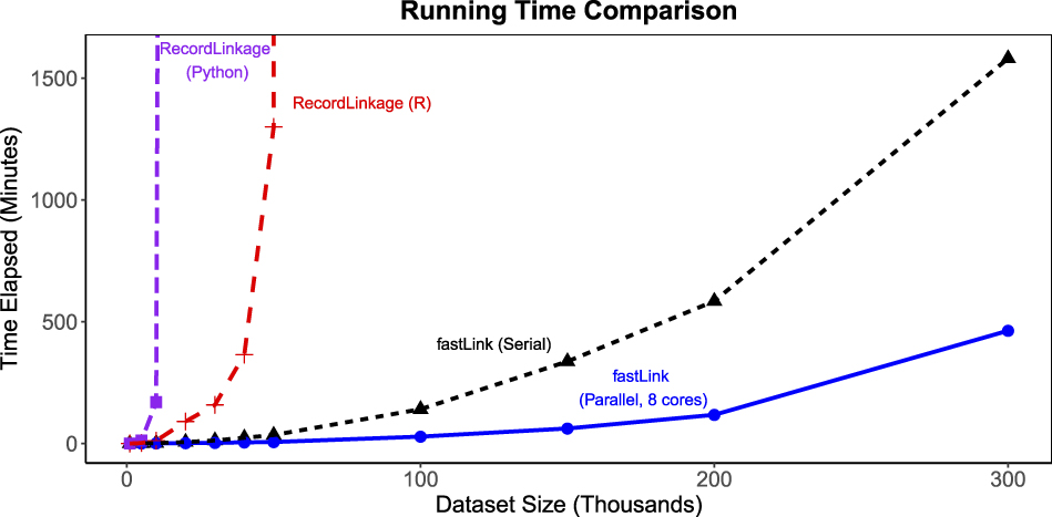


Comments
No Comments have been published for this article.