Local Attentiveness and Policy Representation

In 1977, Fenno wrote that political scientists should focus on studying representatives in the district where “their perceptions of their constituencies are shaped, sharpened, or altered” (Fenno Reference Fenno1977, 883). Understanding how members perceive their constituency is the key to understanding member behavior, as the main goal of a legislator is to get reelected (889). After following 18 congressmen over a period of seven years, Fenno came to the conclusion that members strategically cultivate a unique style in the district depending on constituent preferences. Specifically, a legislator’s home style is composed of how they present themselves to constituents, the allocation of resources between Washington and the district, and explanations of Washington activities (Fenno Reference Fenno1978).

In this paper, I focus on two particularly critical aspects of home style: the allocation of time and staff to the district (Fenno Reference Fenno1977, 891). Both of these resources are important distributive tools that reflect members’ priorities and goals (Parker Reference Parker1986). Although spending time at home takes legislators away from significant Washington activities, such as bargaining with colleagues and drafting legislation, it also allows them to be in the physical presence of constituents. Doing so provides opportunities to cultivate personal relationships and sends the signal that legislators value such interactions. As a result, time in the district is often thought to generate trust and open lines of communication, thereby increasing perceptions of responsiveness and approval (Fenno Reference Fenno1978). Furthermore, time in the constituency provides important opportunities to position take, advertise, and credit claim (Mayhew Reference Mayhew1974).

Locating staff in the district is similarly important, because, as Salisbury and Shepsle (Reference Salisbury and Shepsle1981) argue, “the core of any congressional enterprise is the personal staff of the member” (561). The allocation of staff to state offices reduces legislators’ ability to pursue legislative accomplishments because Washington-based staff are generally dedicated to legislative matters and help legislators write, recruit support for, and navigate legislation through Congress (Montgomery and Nyhan Reference Montgomery and Nyhan2017; Schiff and Smith Reference Schiff and Smith1983). However, doing so also increases the legislator’s ability to connect with constituents, as state-based staff are more accessible and involved in the community. Thus, legislators who allocate more staff to local offices likely have less capacity to pursue legislative accomplishments but more to pursue constituency services. These decisions have been shown to influence constituent perceptions; Parker and Goodman (Reference Parker and Goodman2013) find that senators who spend more on staff and have more state offices are significantly more likely to be viewed as “constituent servants.”

Despite their importance, relatively little is known about how a legislator’s time and staff are allocated throughout the district. Recent research by Walsh (Reference Walsh2012, 517) demonstrates the importance of geographic place and “where that place stands in relation to others in terms of power and resource allocation” in the formation of political preferences. Focusing on the allocation of government economic resources, Walsh (Reference Walsh2012) finds that rural residents favor more limited government due to perceptions of relative deprivation. Although very different, a legislator’s time and staff are also important resources that are often not distributed equally across the geographic constituency. While the question of how legislators decide to allocate their resources has been discussed qualitatively, such as in Fenno (Reference Fenno1998), to my knowledge there has been no empirical analysis of where senators spend their time or locate their local offices. This question is critical to understanding the current state of representation, because it shapes who gets access to their legislators and subsequently how those legislators understand their district.

Legislators may decide to allocate their resources based on a variety of factors. First, they may allocate their time and staff based on population so that they maximize the number of people they reach. Second, senators may consider the location of campaign donors given the high amount of pressure on members to raise funds.Footnote ³ Finally, senators may allocate their time and staff based on electoral competitiveness in an attempt to court swing voters and keep existing supporters happy (Schiller Reference Schiller, Box-Steffensmeier Oppenheimer, Ian and Canon2002). Although these hypotheses are basic theories of one of the most fundamental aspects of representational behavior, they remain untested because there is little systematic data on which subconstituencies are getting selected to receive local resources. Existing studies almost exclusively use measures of the aggregate allocation of resources, such as staffing and visits at the statewide or districtwide level (Lazarus and Steigerwalt Reference Lazarus and Steigerwalt2018; Lee and Oppenheimer Reference Lee and Oppenheimer1999; Parker Reference Parker1986), to investigate legislator behavior. As a result, scholars have been unable to determine where these resources are located within a district and their effects on policy representation.

Classic works such as Fiorina (Reference Fiorina1977b) suggest pessimism about the relationship, arguing that members use ever-increasing staff to distract constituents from what is truly going on in Washington. If legislators focus on credit claiming, constituents may not notice or care that they aren’t being substantively represented. Similarly, Grimmer (Reference Grimmer2013) demonstrates that legislators from politically heterogeneous districts emphasize appropriations in their communications with constituents as opposed to policy positions. This strategy downplays policy disagreement and highlights the local activities of legislators, which can appeal to constituents across the ideological spectrum. As a result, “representatives may be able to use their home styles to generate leeway for their out-of-step views and decrease the information about roll-call votes in Washington” (Grimmer Reference Grimmer2013, 16).

District activities can also substitute for policy representation by providing the legislator with a vehicle for cultivating trust among constituents. In contrast to the idea of legislators distracting constituents with local benefits, cultivating trust requires the legislator to explain their behavior in Washington (Fenno Reference Fenno1978). These explanations include defenses of policy positions and often involve “running for Congress by running against Congress” (Fenno Reference Fenno1978; Lipinski, Bianco, and Work Reference Lipinski, Bianco and Work2003). Lipinski, Bianco, and Work (Reference Lipinski, Bianco and Work2003) find that these distancing explanations can have positive electoral consequences for members of the House with disaffected voters. Similarly, Grose, Malhotra, and Parks Van Houweling (Reference Grose, Malhotra and Van Houweling2015) show that, while senators do not hide their votes on key roll calls from constituents with whom they disagree, they do “tailor aspects of their messages to the views of the person” they are attempting to convince (725). The authors go on to show that these tailored explanations are effective at increasing support for the incumbent, suggesting that a legislator who spends more time convincing constituents to trust them should gain more voting leeway in Washington.

However, although legislators may be able to build trust through carefully crafted communications, spending time on the ground is a very different sort of interaction for which we have little empirical data. For example, face-to-face interactions do not allow legislators to take their time and tailor the perfect response. Instead, district events, such as town halls, are uncontrolled environments that require legislators to think of responses to pointed questions on the fly. Furthermore, in contrast to the control legislators have over the topics of press releases and other constituent communications, they do not get to pick which issues constituents bring up in discussion. It is difficult to opt out of an exchange, forcing legislators to address issues they may otherwise choose to brush under the rug.

Additionally, there are reasons to believe that a senator’s time and staff are particularly ill-suited to work as substitutes for policy representation in today’s political environment. Congress is currently more polarized than ever before, and affective polarization is at an all-time high (Iyengar and Westwood Reference Iyengar and Westwood2015; McCarty, Poole, and Rosenthal Reference McCarty, Poole and Rosenthal2016). While appropriations normally fund public goods that benefit all constituents in an area, a senator’s time and staff can be used in more targeted ways that may serve to alienate constituents who do not feel that their priorities are being represented. Similarly, research has shown that constituents are significantly more likely to reach out to copartisan representatives for help, limiting the benefit of local staff for out-party constituents (Broockman and Ryan Reference Broockman and Ryan2016). As a result, while expanded constituency service opportunities may have been behind the rising incumbency advantage of the 1960s (Fiorina Reference Fiorina1977a), increasingly polarized and nationalized politics has made for a very different contemporary electoral environment (Jacobson Reference Jacobson2015). District activities may no longer serve as effective substitutes for policy representation, but instead work in a complementary fashion to build support among followers and dampen support among the opposed.

With this in mind, I propose an alternative theory in which cultivating a local presence has polarizing consequences for constituents. When a legislator spends more time at home or allocates more staff to an area, they increase the salience of their record, including their policy positions. For example, it has been shown that constituents who participate in e-townhalls with their representative are more likely to become informed about the topic of discussion (Esterling, Neblo, and Lazer Reference Esterling, Neblo and David2011). Local activities can invite greater scrutiny of a senator’s voting behavior or potential behavior due to higher constituent exposure, leaving the senator more popular among constituents who agree with the senator’s positions and less popular among those who don’t. This suggests that local activities give senators’ less leeway to vote how they want in Washington. Consequently, district activities may actually strengthen issue accountability between legislators and their constituents by making constituents more aware of their senator’s behavior in Washington.

In this vein, numerous studies suggest that district activities and policy representation should actually work as complements. Ansolabehere and Snyder (Reference Ansolabehere and Snyder2000), Groseclose (Reference Groseclose2001), and Stone and Simas (Reference Stone and Simas2010) all demonstrate that candidates with valence advantages will locate in the middle of the ideological spectrum. The combination of a valence advantage, such as perceptions of competence, and the ideological advantage from locating at the median voter work together to ensure that the incumbent will beat the challenger. If this is true, senators should use district activities, which can generate such perceptions (Fiorina and Rohde Reference Fiorina, Rohde, Fiorina and Rohde1991), and policy representation together in a complementary fashion. Discovering whether these two dimensions of representation work as complements or substitutes is an important question, as it speaks to questions of accountability and representational quality. As explained by Stone and Simas (Reference Stone and Simas2010), “if a valence advantage by one candidate over the other creates the opportunity and incentive to shirk, the two dimensions of representation work at cross purposes. On the other hand, if constituents’ interests in nonpolicy and policy concerns reinforce the quality of representation on both dimensions, there is cause for optimism about the electoral process” (371).

Serra and Moon (Reference Serra and Moon1994) come the closest to an ideal study by working with a congressional office to get the actual names of constituents who benefited from casework. They then compare the ideology of these constituents with the incumbent and predict voting outcomes, finding that constituents do not consider casework to be a substitute for policy representation. While suggestive, further analysis is required in order to extrapolate beyond a single congressional district. In the following sections, I analyze senator behavior at the county and metropolitan statistical area level, allowing for the first comprehensive observational test of the relationship between home style and policy representation.

Home Style in the Senate

This paper focuses on the Senate because there is very little known about senator resource allocation, and the size of the districts, which are entire U.S. states, provide important leverage over the question of how legislators decide to allocate their resources across their constituencies. However, studies of representation and resource allocation have largely focused on the House. The House, which is the larger of the two congressional bodies, provides the opportunity to study many members who are in charge of representing relatively small and homogeneous congressional districts. Numerous studies including Fiorina and Rohde (Reference Fiorina, Rohde, Fiorina and Rohde1991), Adler, Gent, and Overmeyer (Reference Adler, Gent and Overmeyer1998), Ansolabehere, Snyder, and Stewart (Reference Ansolabehere, Snyder and Stewart2000), and Tucker (Reference Tucker2020) have provided insight into how members of the House cultivate local reputations and the subsequent electoral repercussions. In contrast, the Senate has received substantially less attention. Designed to be less parochial, the Senate is often thought of as being above the local politics that home style requires. As explained in Federalist 62, the upper chamber was created to avoid “the impulse of sudden and violent passions,” and therefore be more distant from the general public (Madison, Hamilton, and Jay Reference Madison, Hamilton and Jay2009). While the Senate has now been directly elected for over a century, it still has a culture of independence and six year terms intended to insulate members from constant electoral pressure. As a result, it has been questioned whether the canonical theories of home style can be applied to the Senate, or whether senators cultivate home styles at all.

Fenno (Reference Fenno1981; Reference Fenno1998) and others argue that senators do in fact cultivate home styles, with some important differences from House members. For example, it has been shown that senators have different home styles and campaign styles thanks to longer six year terms (Fenno Reference Fenno1981), that senators are less dependent on spending time in the district thanks to frequent media attention from large outlets (Fenno Reference Fenno1981; Sinclair Reference Sinclair1990), and that state size is an important source of heterogeneity in senatorial home style (Lee and Oppenheimer Reference Lee and Oppenheimer1999). While these factors remain constant, Parker (Reference Parker1986) reports that changes in travel subsidization and legislative scheduling led to significant increases in attentiveness between 1958 and 1980, suggesting that disparities in attentiveness may change over time with the rules and norms of the legislature.

Unfortunately, the study of how these local behaviors have carried over into the twenty-first century has been limited due to data availability. Members of Congress do not make their calendars public, leading most studies to measure how legislators allocate their time via the amount of money spent on travel or the total number of days spent at home (Bond Reference Bond1985; Lazarus and Steigerwalt Reference Lazarus and Steigerwalt2018; Parker Reference Parker1986; Parker and Goodman Reference Parker and Goodman2013). Although this measure captures how a legislator prioritizes travel in comparison with other activities, it does not provide information on where legislators actually go. Measuring constituency service has also proven difficult. It is almost impossible to get accurate measures of casework over time, as congressional offices have incentives to keep constituent information private and overestimate how many constituents they’ve helped (Cain, Ferejohn, and Fiorina Reference Cain, Ferejohn and Fiorina1987).Footnote ⁴ In order to get around this issue, studies often rely on survey questions in which respondents are asked to recall interactions with their representatives.

While such measures have made important headway in analyzing how the home style of senators influences constituent impressions, little is known about the local nature of these decisions and their subsequent effects on representation. Furthermore, beyond the intralegislature changes analyzed by Parker (Reference Parker1986), improvements in transportation and a shifting media environment may have also changed the calculus of resource allocation. Accordingly, further analysis is required to determine whether modern day senators cultivate home styles similarly to those of the past and the consequences for their behavior in Washington.

Data on Local Attentiveness

I investigate two dimensions of local attentiveness. First, I analyze the amount of time a senator spends among constituents, measured by local visits. Second, I explore the allocation of congressional staff, measured by the percentage of staff placed in local offices. In this section, I detail the data collection process and summarize these measures.Footnote ⁵

Local Visits In order to capture how legislators spend their time at home among constituents, I collected senator travel data from Reports of the Secretary of the Senate from April 1, 2011 to December 31, 2018 (the 112th–115th Congresses) with the help of code made public by the Sunlight Foundation (Fenton Reference Fenton2014).Footnote ⁶ These reports are released online biennially and have been publicly available on the U.S. Senate website since 2011.

Reports of the Secretary of the Senate provide in-depth records of how senators use their Senators’ Official Personnel and Office Expense Accounts, which are calculated based on state population and distance from Washington DC.Footnote ⁷ The average senator gets about $3.7 million and can use this money as they wish to pay for official expenses, which are labeled by category in the reports.Footnote ⁸ In order to determine where senators are actually spending their time interacting with constituents, I collect all items labeled as being part of a senator’s “per diem.”Footnote ⁹ The “[p]er diem is the allowance for lodging (excluding taxes), meals and incidental expenses,” (U.S. General Services Administation 2020) leading it to capture where senators are eating, drinking, and sleeping when they are traveling the state.

Using these data, I collect each time a senator uses his or her per diem and match the listed places to the appropriate county.Footnote ¹⁰ I analyze visits to counties because it is the most localized level possible that allows me to connect the data to the appropriate survey responses. Further, Fenno (Reference Fenno1977) often recounts members discussing their districts in terms of groups of counties, suggesting their importance to the conceptual grouping of constituencies. However, an event in a major city may also affect the constituents living in surrounding counties. As a result, I therefore also perform all analyses at the metropolitan statistical area (MSA) level. MSAs are groups of counties with a core area that are economically and socially connected. Specifically, each MSA must have at least one urban area of 50,000 or more people, leading this measure to account for a more limited number of places but ones that are connected to population centers likely to be often visited by senators.Footnote ¹¹ Additionally, although counties can vary greatly in size, MSAs are more comparable across states. I use the number of visits to each place in a county or MSA as a measure of constituent exposure, as opposed to the length of a trip, because the per diem receipts often only list the start and end dates of the entire trip.

In a given year, the average county gets a combined 1.5 visits from both senators. Further, 53% of the population lives in a county that gets visited. Figure 1 displays visits to counties over the entire period of the data. The variable is logged to account for the right-skewed nature of the data. Clearly, there are some counties that are getting dramatically more interactions with their legislators than others. For example, visits are relatively evenly distributed across the counties in Wyoming, but there is a much larger amount of variation in other states such as California and Texas. This suggests both differences between states and within states, leading to varying abilities of constituents in these areas to interact with their legislators.

Figure 1. Senator Trips to Counties

These data provide the opportunity for a highly localized analysis of senator travel patterns. To illustrate this, Figure 2 displays the travel patterns of two senators from Wisconsin: Senator Tammy Baldwin (D-WI) and Senator Ron Johnson (R-WI).

Figure 2. An Example of Partisan Variation in Travel Patterns

The clearest pattern is that both senators travel to where they live. Senator Baldwin lives in Madison, and Senator Johnson lives in Oshkosh. Second, Senator Baldwin almost never travels to western Wisconsin, which is a Republican stronghold. However, she did do so in 2017, the year before effectively flipping many rural areas toward her favor in the 2018 election. Senator Johnson can also be seen traveling to the northern Democratic areas of Wisconsin in the year of his election. Finally, both senators make a significant number of trips to the Milwaukee area, which contains the largest city in the state and went for Hillary Clinton in the 2016 presidential election. These patterns suggest that the senators take different approaches to traveling their home state, although not ones that can be completely explained by partisanship.

While this dataset provides important insights into senator travel patterns, it also has some drawbacks. Most importantly, there is missingness in the data. Some senators do not list any per diems in certain years, leading there to be around 20 to 30 senators with no per diems listed for a given year of the data. While it is possible that these senators are simply not traveling around their state, in which case these observations would be true zeros, this is likely not always the case. This missingness would cause problems for making inferences if it is correlated with the outcome of interest. I investigate whether the causes of missingness are observable by both analyzing the data and speaking to actual staffers and one senator. I then use numerous strategies to address this issue.

First, I run a model using time-varying senator characteristics to predict whether or not a senator reports any per diems in a given year. The results can be seen in Table A.1, and they suggest that committee chairs and more senior members are significantly more likely to report per diems. Congressional leaders may feel the need to set an example for the party or have more reliable staff. Additionally, senators are less likely to report per diems when they are running for reelection. This is unsurprising, given that senators are not allowed to use their official allowances for campaigning. As a result, in the following analyses I control for chairmanship, seniority, and whether or not the senator is running for reelection. The third variable predicting missingness is state size. Senators from small states are significantly less likely to report per diems than senators from large states. To address this concern I include senator fixed effects, which hold such time-invariant factors constant in the analyses. Finally, I replicate the analyses using transportation receipts instead of per diems. Although these receipts are more noisy than per diems because they mostly report places with airports, they also suffer from less missingness.

Local Offices I collected data on where senators choose to locate their local offices and how many staffers they dedicate to them using the Senate Telephone DirectoryFootnote ¹² for the period of 2011 to 2018 (the 112th–115th Congresses). Although each senator is authorized office space in federal buildings, such office space is not always available (Brudnick Reference Brudnick2018). Furthermore, there is no restriction on the number of offices that they may have or input on how they should divide their staff.

Once again, these data allow for a uniquely detailed analysis. In a given year, 7% of counties have an office, containing about 43% of the population. The average county with an office gets allocated 7.3% of a senator’s total staff. Figure 3 displays the location of all local offices included in the sample, with shaded counties representing locations with at least one office.Footnote ¹³ Continuing the example from Figure 2, Figure 4 displays the location of state offices for Tammy Baldwin and Ron Johnson over the entire period of the data. Although some of the locations overlap (such as Dane County, which contains the capital city), the allocation of resources to these areas vary.

Figure 3. The Location of Staffers

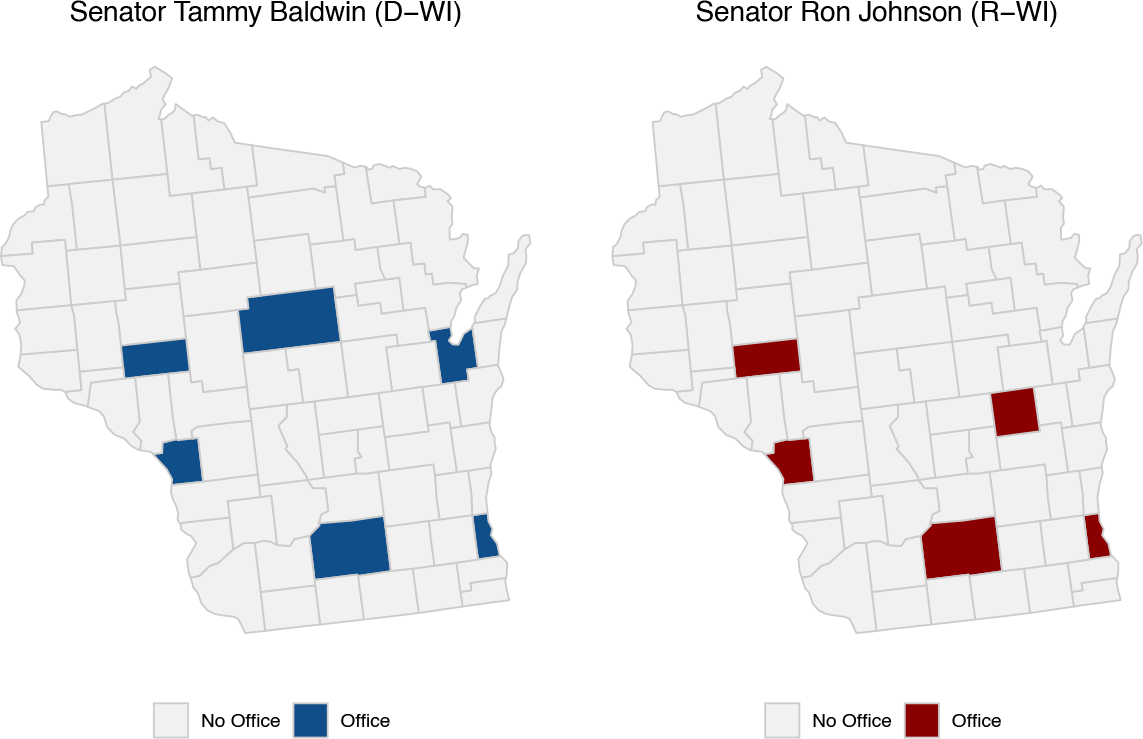
Figure 4. An Example of Partisan Variation in Staffing Patterns

In the following sections, I first use these measures as dependent variables in an analysis to determine how senators decide where to allocate their resources across the constituency. Second, I use them as independent variables to assess whether or not such resources can be successfully used as tools to gain legislators voting leeway in Washington. Taken together, these analyses provide new insights into both the distribution of resources and the subsequent consequences for the legislator–constituent relationship.

The Geographic Allocation of Resources

All senators need to decide how to distribute their resources across the constituency. Although this question has been discussed qualitatively, such as in Fenno (Reference Fenno1998), to my knowledge there has been no empirical analysis of where senators spend their time or locate their local offices.Footnote ¹⁴ In order to answer this question, I use the characteristics of a county and MSA to predict the extent to which a Senator visits and staffs an area.Footnote ¹⁵ In doing so, I hope to provide descriptive information about senator resource allocation patterns. I include four categories of independent variables, including electoral competitiveness, campaign donations, population size, and local demographics.

The first category of variables captures electoral competitiveness, with all data on Senate elections coming from Leip (Reference Leip2018).Footnote ¹⁶ While all legislators seek to get reelected (Mayhew Reference Mayhew1974), it is unclear whether senators expend more effort courting voters in competitive areas or instead focus their resources on core constituencies. Analyzing how presidents allocate federal dollars across geographic constituencies, Kriner and Reeves (Reference Kriner and Reeves2015) find that core counties located in core and swing states received significantly more federal funding than similar counties in opposition states. In order to determine whether senators also behave in this way, I create indicators for whether an area is a “core” or “swing” area. Following their operationalization, a county/MSA is counted as a core area if the senator received at least 55% of the vote in the previous election. An area is considered a swing area if the senator received between 45% and 55% of the vote in the previous election.Footnote ¹⁷

The second category focuses on campaign contributions. The work of Kalla and Broockman (Reference Kalla and Broockman2016) suggests that contributions facilitate access to legislators, leading to the expectation that senators will place greater resources in areas with a higher concentration of donors. For example, in the 114th Congress Senator Rob Portman (R-OH) visits both Beachwood and Chagrin Falls, Ohio. Although both of these places are small (less than 12,000 people as of the 2010 census), they are donation powerhouses—both are listed as top donation zip codes to Senator Portman in the year of his election in 2016 (Open Secrets N.d.). In order to empirically investigate the relationship between donations and access to resources, I include an indicator for whether individuals in the area contributed greater than individuals in the average area within the state to the senator’s party in the previous presidential election.Footnote ¹⁸ I focus on presidential elections to capture the pool of possible donors in an area. These data come from Bonica (Reference Bonica2019).

The last category consists of population size. I expect population to be a positive predictor of visits, as large and urban areas often have greater political power than small and rural areas due to the presence of media outlets, business hubs, and potential voters. Finally, I include percentage of white and median household income as additional controls, with census data collected from the American Community Survey.Footnote ¹⁹

These independent variables, which are further described in Table 1,Footnote ²⁰ are then used to predict the relevant dependent variable in Table 2. Because the dependent variables of interest are heavily zero inflated, I present three different regressions. Column 1 uses the binary version of the dependent variable, where a one represents whether the area received any resources. Column 2 uses the raw version of the dependent variable, which is total resources allocated to an area. Column 3 uses the logged version of the dependent variable (plus one) in order to account for the skewed nature of the data. All models include year and senator fixed effects, allowing me to analyze within-senator changes in attentiveness while controlling for year-specific trends. As a result, tendencies specific to certain senators, such as one’s hometown, will be held fixed. In addition to the main variables of interest, I also use data from Volden and Wiseman (Reference Volden and Wiseman2020) and Stewart and Woon (Reference Stewart and Woon2017) to control for whether the senator is running for reelection, chamber seniority, chairmanship, majority party status, and whether the member is on a top committee. Finally, I include indicators for whether the area contains the capital city and has an airport with a direct flight from DC.Footnote ²¹ Standard errors are clustered on senator.

Table 1. Predictors of Senator Resource Allocation

Table 2. The Relationship between Local Characteristics and Senator Resource Allocation

Note: Entries are linear regression coefficients with standard errors (clustered on senator) shown in parentheses. The dependent variables are various transformations of the number of resources a senator allocates to an area. *p < 0.10, ^**p < 0.05 (two tailed tests).

Table 2 displays the results. Columns 1 through 3 display the results for local visits, and columns 4 through 6 display the results for local staff. The top panel shows the results for counties and the bottom panel for MSAs. First, neither Core Area nor Swing Area is a significant predictor of trips to counties. This aligns with what I was told by the administrative director of a former senator, who suggested that some senators try to visit every county in the state in a given year. However, the coefficient on Core Area is significant at the MSA level. Specifically, going from an opposition area to a core area is associated with one additional visit. There is stronger evidence that senators are acting strategically in other ways. The coefficient on Above Avg. Donations is positive and significant across all regressions. This finding bolsters the work of Kalla and Broockman (Reference Kalla and Broockman2016), as it appears that providing a high amount of donations significantly increases an area’s access to senators. The coefficient on Log Population is also consistently positive and significant. The finding that senators are going to highly populated areas suggests that they are trying to reach the most people possible. Finally, Median Household Income and Percent White tend to be negative across specifications.Footnote ²²

The results for local staffing patterns tell a somewhat different story. Core Area is consistently a positive and significant predictor at both geographic levels, indicating that senators place more staff in core areas as opposed to opposition areas. Swing areas are also significantly more likely to get staff than opposition areas, although the significance is more inconsistent and coefficients tend to be smaller. This result suggests that staff is a more similar resource to federal funding than time, as its allocation is more sensitive to previous electoral performance. Similarly, Above Avg. Donations to Party is also a positive and significant predictor, once again indicating the outsize influence that donating provides to constituents. More populated areas also have more access. According to my conversations with staff, senators attempt to spread out their state operations to try and reach as many constituents as possible, although the location of federal buildings also plays a role. Finally, the coefficients on Median Household Income and Percent White are negative across specifications. Staffers tend to be placed in areas with more low income and nonwhite constituents.

Overall, senators allocate both of these resources to follow people and money, suggesting that home style may now be driven by the increased pressure to raise funds. The average cost of winning a Senate seat in 2018 was $15.7 million, requiring senators to now participate in the “constant campaign” they were meant to be insulated from.Footnote ²³ Areas with important donors are getting the most face time with senators and their staff, suggesting a so-far unexplored consequence of increasing levels of money in politics.

Local Attentiveness and Ideological Agreement

How do these patterns interact with the roll-call voting behavior of senators? Traditional theories of home style suggest that senators use district activities to gain voting leeway in Washington (Fenno Reference Fenno1978; Grimmer Reference Grimmer2013), decreasing the accountability of legislators to their constituents. However, an increased presence at home may increase the salience of a legislator’s policy positions, therefore decreasing leeway and increasing accountability. In order to adjudicate between these competing theories, I test the hypothesis that constituents are more likely to approve of ideologically out-of-step incumbents in areas that receive more attention.

This idea is inspired by Canes-Wrone, Brady, and Cogan (Reference Canes-Wrone, Brady and Cogan2002), who show that roll-call decisions affect the electoral fates of incumbents. They find that House incumbents receive lower electoral margins the more they vote with the extreme end of their party, suggesting that ideologically out-of-step incumbents are punished by constituents. Under the theory that incumbents use district activities and roll-call votes as substitutes, incumbents should act to alleviate the punishment for being out-of-step by spending time in a county shaking hands, explaining their votes, or dedicating staff to the area. According to Fenno (Reference Fenno1978), this behavior works to build trust among constituents, which in turn allows the representative independence in the legislature. Constituents who ideologically disagree with the incumbent in these areas should then be more likely to approve of the incumbent than they otherwise would be. Alternatively, constituents may be more likely to approve of out-of-step incumbents in areas that receive less attention. Visits and staff may work to exacerbate differences or call attention to them, leading these resources to be more efficiently used elsewhere, such as among supporters.

Following the lead of Ansolabehere and Kuriwaki (Reference Ansolabehere and Kuriwaki2021), I measure ideological agreement by connecting survey responses to questions asking respondents whether they support or oppose specific pieces of legislation or a policy in the Cooperative Congressional Election Study (CCES; Kuriwaki Reference Kuriwaki2018) and match them to actual floor votes in that Congress. Using the 2011 to 2018 CCES, I divide the number of times a senator votes against respondent preferences by the total number of votes in question to create the variable Policy Disagreement. Footnote ²⁴ While some years of the CCES include the corresponding floor votes, I supplement years that do not with roll-call votes from Lewis et al. (Reference Lewis, Poole, Rosenthal, Boche, Rudkin and Sonnet2021). The issues cover a wide range of topics, such as gun control and education; the full list of CCES questions and roll-call votes used to create the measure are listed in Table D.1. This measure allows me to directly map the opinions of constituents onto the policy actions of legislators. The mean value is 0.44, indicating that constituents agree more with their senators than they disagree. The distribution over time is presented in Figure D.1. I also use the CCES to measure constituent approval of incumbents. Depending on the year, approval is originally asked on a four- or five-point scale. Following Ansolabehere and Rogowski (Reference Ansolabehere and Rogowski2020), I collapse the question to a binary indicator by marking respondents who state that they “strongly” or “somewhat” approve of their senator as approving and the rest of respondents as disapproving.Footnote ²⁵

Accordingly, I regress constituent approval ratings on whether or not the senator traveled to or placed staff in an area.Footnote ²⁶ I interact the relevant independent variable with average policy disagreement. Furthermore, I attempt to address the fact that senators are likely strategically visiting and staffing some areas over others for reasons that could be unobserved or unobservable. This possibility would lead a simple cross-sectional design to incorrectly attribute approval to district focus, as opposed to the true unobservable causes. To do so, I use senator-county/senator-MSA fixed effects, which hold fixed each area’s time-invariant factors with respect to that particular senator constant.Footnote ²⁷ I also include party-year fixed effects to account for variation across years related to partisan trends. If district activities serve as substitutes for policy representation as commonly hypothesized, the relationship should be positive and significant. Alternatively, if they are complements, it should be negative and significant. Finally, I control for other factors that could confound the relationship including copartisan status;Footnote ²⁸ the respondent’s race, gender, and age; whether the senator is running for reelection; and the senator’s chairmanship status, membership on key committees, chamber seniority, and ideology as measured by first dimension Nokken-Poole Scores. Policy disagreement is interacted through the controls, robust standard errors are clustered on senator,Footnote ²⁹ and survey weights are included in all analyses.

Results

The results from this analysis are displayed in Table 3. Once again, I use the binary, raw, and logged version of the independent variable to account for zero inflation. Columns 1 through 3 present the results for local visits and columns 4 through 6 for local staff. The top panel displays results at the county-level, and the bottom panel displays results at the MSA level. Interestingly, the coefficient on the interaction term is negative in all six regressions for local visits, providing suggestive evidence that visits hurt senator evaluations among people who are ideologically distant from them. The coefficient is significant at the 95% level in both the regression using the raw and logged measure of visits at the county level and the raw measure at the MSA level. Specifically, a 100% increase in visits is associated with about a 1–2% decrease in approval. While these results are not overwhelmingly large, there are two reasons to be unconcerned about this. First, their substantive size is in part a consequence of controlling for a significant amount of variation through the use of fixed effects. Second, even if the effect is small, it is still signed in the opposite direction than what the existing scholarship, such as that of Fenno (Reference Fenno1978), suggests it should be. Far from helping legislators build support at home, visits instead appear to hurt them.

Table 3. The Relationship between Local Attentiveness, Policy Representation, and Approval

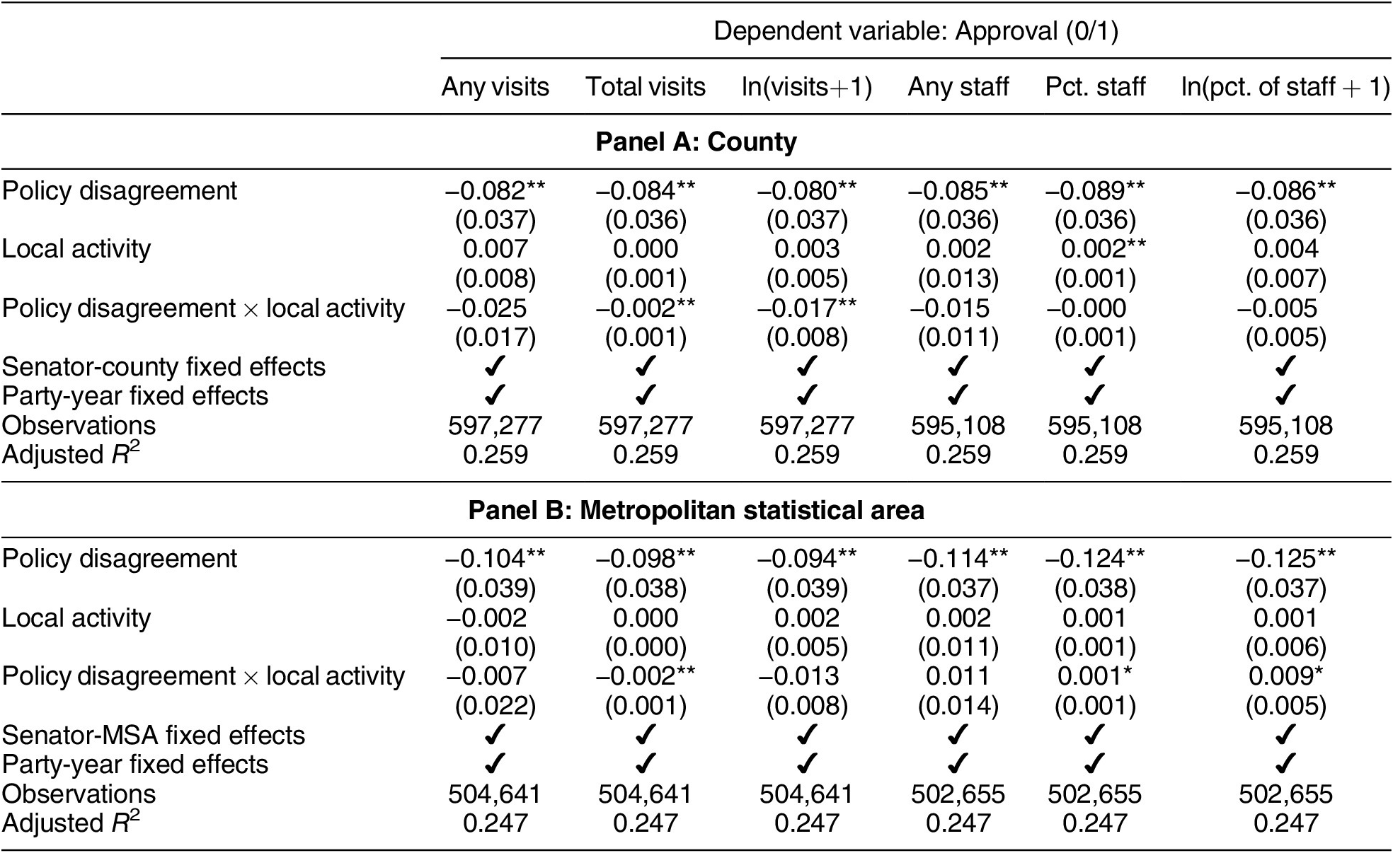
Note: Entries are linear regression coefficients with standard errors (clustered on senator) shown in parentheses. The dependent variable is a binary measure of constituent approval. *p < 0.10, ^**p < 0.05 (two tailed tests).

These results are robust to dropping states with 10 counties or less (Table E.3), dropping senators from Maryland and Virginia (Table E.4), running a model using total visits as the main independent variable while controlling for any visits (Table E.5), and dropping senators who report zero per diems (Table E.6). The results from a regression using transportation receipts instead of per diems can be seen in Table E.7. Although no longer significant at conventional levels, the relationship remains negative at the county level and close to zero. Once again, it does not appear that constituents increase their approval of out-of-step senators when they visit more. Finally, Figure E.1 presents the results from a regression including the lag and lead of any visits in order to test whether senators are strategically visiting areas they know are highly polarized. The interaction on Any Visits This Year × Policy Disagreement remains similar in magnitude and is significant at the 90% level. The coefficients for the previous year’s visits are never significant, suggesting that such strategic behavior is not a threat to inference. Clearly, local visits are not a reliable tool for gaining voting leeway in Congress.

Alternatively, the findings are less suggestive when it comes to the percentage of staffers located in an area. The coefficients on the interaction term are small and inconsistent in direction. Although at the county level none of the interaction terms is significant and all are negatively signed, at the MSA level the interactions for total percentage of staff and logged percentage of staff are positive and significant at the 90% level. Specifically, a 100% increase in the percentage of staff in an area is associated with about a 1% increase in approval. This value seems especially small when considering the cost for a senator to allocate additional staff to an area.

Taken together, these results provide little evidence that local attentiveness bolsters legislators with additional voting leeway. The analysis of local visits reveals a consistently negative, albeit small, effect among constituents in ideological disagreement. Alternatively, while the analysis of staff reveals a potentially positive interaction, the effect is even smaller than that of visits and inconsistently signed. Although these effects are not very large, they provide a striking contrast to the folk wisdom that local activities can be used to build approval among those in ideological disagreement (Fenno Reference Fenno1978).

Local Attentiveness, Policy Disagreement, and Vote Choice

Although analyzing the behavior of senators has many upsides for the purposes of this research question, including the fact that they represent large geographic territories, the downside is that senators are only up for election every six years. As a result of the longer election cycle, the number of available respondents for a vote choice analysis substantially decreases in comparison with the previous analysis of constituent approval. However, it may be the case that although ideologically distant constituents decrease their approval of legislators with more local visits, their actual behavior in the voting booth will remain unchanged. The same could be said for local staffing choices. To investigate this question, I rerun the above analysis using whether or not the respondent states that they prefer to vote for the incumbent.Footnote ³⁰ All respondents who reported intentions to vote for a candidate are included.

The results from this analysis are presented in Table 4 using the logged version of the independent variable.Footnote ³¹ The other transformations are presented in the appendix in Table F.1. Once again, the interaction terms are negative and significant at both the county and MSA level for local visits. A 100% increase in visits is associated with about a 3–4% decrease in the likelihood of voting for the incumbent among constituents in complete disagreement. Interestingly, the coefficients on the interaction terms for staff are both negatively signed, but neither are statistically significant at conventional levels. Finally, it is of note that the base terms on local visits and staff are at times positive and significant. These findings suggest that it is not as though local activity has no potential for positive consequences; they just cannot be used to provide voting leeway as has often been suggested by the literature.

Table 4. The Relationship between Local Attentiveness, Policy Representation, and Vote Choice

Note: Entries are linear regression coefficients with standard errors (clustered on senator) shown in parentheses. The dependent variable is a binary measure of constituent vote choice. *p < 0.10, ^**p < 0.05 (two tailed tests).

What kinds of voters are driving these results? In Table F.2, I rerun this analysis subset by copartisanship. All of the coefficients on the interaction terms remain negatively signed and the relationship is statistically significant among copartisan constituents for visits at both geographic levels. As a result, it appears that local activities fail to garner additional voting leeway among constituents of either group.

Potential Mechanism and Issue Heterogeneity

In this section, I present two final analyses that examine potential heterogeneity in how constituents respond to local attentiveness. The first explores constituent attention to the news and the second investigates variation by issue area. Taken together, these analyses further clarify how local attentiveness and policy disagreement work together to influence constituent evaluations of their legislators.

News Attentiveness While it is possible that constituents are personally attending local events with their senators, it is more likely that they are hearing about them from media outlets. As a result, I expect that the negative effect of local visits should be concentrated among people who report regularly following the news. To this end, I rerun the main analysis subset by whether or not respondents report that they regularly follow what’s going on in government and public affairs. Respondents who say “Most of the time” and “Some of the time” are included as regular news followers. Those who report “Only now and then,” “Hardly at all,” and “Don’t Know” are included as nonregular news followers.

The results are displayed in Figure 5, which shows the 95% confidence interval for the linear marginal effects as well as binned estimates at common levels of policy disagreement. The results confirm the hypothesis that the effect of visits is concentrated among people who follow the news. While there is no effect among respondents who rarely take an interest in the news, the marginal effect of visits is downward sloping and significant at medium and high levels of disagreement for those who do. Overall, these results indicate that local visits do not lead constituents to improve their evaluations of ideologically distant incumbents, and, if anything, they suggest that visits may make them worse.

Figure 5. Potential Mechanism: News Attentiveness

Note: This figure shows linear marginal effects with fixed effects. The model includes senator-county/MSA and party-year fixed effects, with standard errors clustered on senator. The dependent variable is a binary indicator of constituent approval.

Parallel analyses for staff are displayed in Figure H.1. Although it is reasonable to expect that local visits can garner news coverage, it is unlikely that the presence of local staff in an area does. This fact may help to explain why, despite legislators themselves believing in the importance of local staff, they fail to have a large or consistent influence on constituent evaluations. Indeed, the linear marginal effects of the percentage of staff on approval are never significant among regular news followers or nonregular news followers at the county level. However, the marginal effect is positive and significant among constituents who follow the news at high levels of disagreement at the MSA level.

Policy Domain Although the policy disagreement scale includes a wide variety of issues, it is likely the case that constituents are more informed about certain types of policies than others. For example, during this period Supreme Court nominees and the Affordable Care Act received high amounts of news coverage, potentially leading such issues to drive the results. In order to investigate this possibility, I rerun the main analysis subset by issues area for those that were asked about across multiple years. To create the categories, I rely on The Policy Agendas Project coding of Senate roll-call votes into major topics (Comparative Agendas Project 2019).Footnote ³² The results for visits are presented in Figure 6. Although the majority of coefficients are negatively signed, a few issues stick out as being particularly influential. First, the coefficients on the interaction term for energy issues are negative and significant at both the county and MSA levels. This category is made up of votes about the Keystone Pipeline, a particularly divisive topic. Second, votes on health policy also appear to have a strong effect. These votes concern repealing the Affordable Care Act, exemptions for employers from providing their employees with birth control, and Medicare policy. Finally, the coefficient for macroeconomic issues is just above significance at the 90% level for counties. These votes center on raising the debt ceiling and middle class tax cuts.

Figure 6. Analysis by Issue Area

Note: The figure presents the linear regression coefficients on the interaction of “Policy Disagreement” and “ln(local visits + 1)” with standard errors clustered on senator. Vertical lines are the 90% and 95% confidence intervals associated with the estimated effects. The horizontal dashed line is the null hypothesis of no effect.

Parallel analyses for staff are displayed in Figure H.2. Energy and macroeconomic issues once again stand out as consistently negative. The coefficients for issues regarding international affairs and foreign aid are also negative and statistically significant.