


Sick of elecshun [sic] related violence and terror attacks. Can’t wait for elecshuns to be over and get non-elecshun related violence back.
—A tweet from the satirical and pseudonymous@majorlyp during the 2013 Pakistani elections
A prominent argument for democracy centers around the fact that elections allow political groups to compete via ballots rather than bullets. However, elections are often violent affairs. Conflict surrounding the 2007 elections in Kenya led to around a thousand deaths and hundreds of thousands displaced. Similarly, dozens were killed in the May 2013 election-related violence in the Philippines. More generally, electoral violence is not a new phenomenon nor limited to nascent democracies, but a problem “virtually all states have experienced” (Rapoport and Weinberg Reference Rapoport and Weinberg2000, 42). As many Western governments and NGOs at least nominally encourage other countries to hold elections, the question of whether doing so incites violence is of great practical as well as theoretical importance.
That elections are a necessary condition for electoral violence is tautological; of greater interest is how elections affect patterns of political violence more generally. Still, recent empirical studies have found that various forms of political violence sometimes do spike around elections (e.g., Aksoy Reference Aksoy2014; Hafner-Burton, Hyde, and Jablonski Reference Hafner-Burton, Hyde, Ryan and Jablonski2014; Newman Reference Newman2013). Figure 1 illustrates this pattern for several African countries in a way that will relate closely to our theoretical model. Each panel shows yearly counts of violent events in a country from the Social Conflict Analysis Database (SCAD) for 1990–2010 (Saleyhan et al. Reference Salehyan, Hendrix, Hamner, Case, Linebarger, Stull and Williams2012) with vertical lines illustrating years with elections where the chief executive office was at stake (Hyde and Marinov Reference Hyde and Marinov2012). Kenya illustrates the pattern we seek to explain starkly: in three out of four years with elections, there were more violent events than the years before and after. Ghana experienced similar spikes in violence around elections in 2000 and 2008, though the most violent year was the one preceding an election (1995). In Burkina Faso, the largest spike of violence occurred in the year following an election, while in Nigeria patterns in violence seems unrelated to election years.

FIGURE 1. Counts of Violent Events for Select African Countries by Year, with Vertical Lines at Years with Elections where the Office of the Incumbent was Contested
A clearer view of this “political violence cycle” emerges when aggregating across countries and taking a more fine-grained time window. Figure 2 presents the average daily level of violence from a month before to a month after election day, for elections where the office of the incumbent leader was (left panel) and was not (right panel) at stake, using the full sample of SCAD (which includes Latin America in addition to Africa). Two patterns readily stand out: first, there is a cyclical pattern with a clear spike in violence around the day of the election for both types of elections. Second, there is a higher (average) level of violence around elections when the incumbent leader’s office was in contention. (See the Appendix for a complete description of the data and procedures that generate these graphs.)

FIGURE 2. Average Counts of Ongoing Violent Events by the Number of Days to the Closest Election for Full Sample of SCAD
Motivated by patterns like this and the association between elections and violence more generally, some have suggested that promoting elections could be dangerous in certain contexts (Brancati and Snyder Reference Brancati and Snyder2012; Collier Reference Collier2009; Flores and Nooruddin Reference Flores and Nooruddin2012). More frequently, scholars of the relationship between elections and violence do not advocate against holding elections, but do express a clear unease that their results could be used to make such an argument.Footnote 1 And these fears are not unfounded: those writing for more general audiences have used this association to discourage democracy promotion, e.g., calling elections or democracy more broadly a “curse” (Economist 2013) or “among the causes of both the Rwandan and Yugoslavian genocides” (Chua Reference Chua2004, 12).
We provide a simple and general formal argument which demonstrates that spikes of violence during elections cannot be used as evidence that elections make politics more violent on average.Footnote 2 The crux of our argument is that elections affect incentives to use violence to further political objectives not only leading up to and directly after the voting, but at all times. In particular, the presence of an election in the future can decrease incentives to commit violence today precisely because violence—as well as nonviolent political action—become more effective during electoral periods. That is, making electoral violence a more effective tool to change political outcomes has a direct effect of increasing violence surrounding elections, but this can be partially if not fully offset by an indirect effect of decreasing violence in the periods between elections. So, we cannot conclude from this evidence that elections—or more consequential elections—make politics more violent.
Our theoretical argument has important implications for the empirical study of electoral violence. The strategic use of violence around elections and associated temporal dynamics makes empirical assessment of how elections affect total violence levels extremely difficult, since it involves constructing the counterfactual of a world with less consequential elections or none at all. For example, when observing a country where violence increases during elections, it is tempting to conclude that politics would have been more peaceful without elections. However, the increase in violence could be driven by the direct effect or indirect effect described above (or both).
To allow for such counterfactual comparisons (albeit theoretically), we develop a series of formal models which generate dynamics similar to the empirical record with elections, and then ask what would happen were elections to become less consequential or nonexistent. In our main model, two parties compete over the spoils from holding office, and the party in opposition commits violence in an attempt to oust the incumbent.Footnote 3 To set up a “hard case” for elections to have a pacifying effect, we take it as a given that violence is more effective in electoral periods, in the sense that a marginal increase in the opposition’s violent effort has a higher impact on their chance of taking over office. Consistent with Figures 1 and 2, this simple setup generates a political violence cycle, where conflict peaks in electoral periods. However, the presence of elections decreases the amount of violence in nonelectoral periods compared to a baseline where elections never happen. When the indirect effect of reducing violence in nonelectoral periods outweighs the direct effect of increasing violence during electoral periods, the average level of violence is lower in a society with elections than in the counterfactual without elections. So, our first main result is that even when assuming that the only thing elections do is periodically make violence more effective, the overall impact of elections can be to make politics more peaceful.
Our second main result is that a similar cyclical pattern of violence can arise if elections also provide a nonviolent means to contest for power and unambiguously make society more peaceful. To demonstrate this, we allow the opposition to also take nonviolent actions to increase their chance of taking office during electoral periods (e.g., campaigning). Providing this alternative means of contesting for power lowers the level of violence in electoral periods as well as the periods leading up to elections for a similar reason described above; there is less incentive to commit violence leading up to an electoral period when parties can wait until they are able to contest for power peacefully. If the relative cost of nonviolent political activity is sufficiently low, there will always be less violence in a political system with elections; in fact, there may be less violence in every period compared to a baseline without elections. Further, when the nonviolent activity is sufficiently effective, peaks of violence can occur after the election, consistent with the prevalence of postelection protest, particularly in less-than-democratic countries (Daxecker Reference Daxecker2012; Rozenas Reference Rozenas2012; Hyde and Marinov Reference Hyde and Marinov2014).
Finally, we conduct two additional extensions to demonstrate that the central arguments of the article apply to violence committed by different actors and with different goals. First, we allow the incumbent to commit violence, which shows that our model can also capture the (often more empirically relevant) incidence of violence perpetrated by government forces. Similar results hold even if the incumbent commits the vast majority of violence. Second, we consider violence used to attain more incremental political objectives than taking over office, which also leads to a similar cycle of violence around elections that can make society more or less peaceful on average. In sum, the models suggest that political violence committed by any actor for any purpose can follow a cyclical pattern peaking at election time without implying that there would be less violence of this form without elections.
RELATED WORK
Holding regular elections is central to democracy since it provides a mechanism through which societal differences are peacefully resolved and voters can hold their representatives accountable for their actions (Przeworski Reference Przeworski2005; Przeworski, Stokes, and Manin Reference Przeworski, Stokes and Manin1999; Schumpeter Reference Schumpeter1942). However, a growing literature on when and why violence is used during elections has challenged this idea by showing the link between the central instrument of democracy and conflict.
The existing theoretical literature on electoral violence primarily analyzes how elites use violence around elections to improve their chances at the polls. For example, Ellman and Wantchekon (Reference Ellman and Wantchekon2000) present a model on how threats of violence influence policy choices of different parties. Similarly, Chaturvedi (Reference Chaturvedi2005) shows how elites use violence to influence both voter turnout and vote choice. In a similar vein, Collier and Vicente (Reference Collier and Vicente2012) argue that in situations where violence is effective in swaying swing voters, some types of incumbents and challengers will use repression and terrorism, respectively. However, these models do not examine how elections affect incentives to commit violence in nonelectoral periods or what would happen in the absence of elections, so they tell us little about how elections affect patterns of political violence more generally.
Other recent game-theoretic work compares levels of violence in a game with and without elections, but only in a single period (Cox Reference Cox2009; Little Reference Little2012). In many existing formal models, elections always reduce violence as—loosely speaking—voting or elections act as substitutes for fighting (Fearon Reference Fearon2011; Przeworski, Rivero, and Xi Reference Przeworski, Rivero and Xi2012), the election fully alleviates the uncertainty that can cause bargaining to break down (Cox Reference Cox2009), or reducing antigovernment violence is the goal of elections (or democratizing) and hence they are only held when serving this end (Acemoglu and Robinson Reference Acemoglu and Robinson2000; Little Reference Little2012).
A considerable empirical literature supports the more skeptical theoretical models. For instance, Hafner-Burton, Hyde, and Jablonski (Reference Hafner-Burton, Hyde, Ryan and Jablonski2014) show that incumbents will use violence during electoral periods when she fears losing power or when there are institutionalized constraints, but that this may also lead to risky postelection violence (Hafner-Burton, Hyde, and Jablonski Reference Hafner-Burton, Hyde and Jablonski2015).Footnote 4 Similarly, Aksoy (Reference Aksoy2014) shows that electoral violence is more likely in places with low “electoral permissiveness.” Both Wilkinson (Reference Wilkinson2004) and Brass (Reference Brass2003) describe how Indian elites use violence to increase the turnout of their supporters and decrease that of the challengers. Using data from Africa, Daxecker (Reference Daxecker2012) argues international monitoring of flawed elections can raise the salience of fraud and consequently the risk of postelection violence, and Kasara (Reference Kasara2015) shows how violence may also influence future (and not just upcoming) elections in Kenya. Elections may be particularly dangerous in countries that have recently transitioned from an autocracy to a democracy (Cederman, Hug, and Krebs Reference Cederman, Hug and Krebs2010; Collier Reference Collier2009), or that have recently recovered from conflict (Brancati and Snyder Reference Brancati and Snyder2012; Flores and Nooruddin Reference Flores and Nooruddin2012; Reilly Reference Reilly2002).Footnote 5
Most directly related to our model is a burgeoning empirical literature which focuses specifically on spikes in violence, repression, and terrorism during electoral periods (Bekoe Reference Bekoe2012; Goldsmith Reference Goldsmith2014; Newman Reference Newman2013; Norris, Frank, and Martinez i Coma Reference Norris, Frank and Martinez i Coma2015; Staniland Reference Staniland2015). The types and perpetrators of violence may also change surrounding elections: e.g., Straus and Taylor (Reference Straus and Taylor2012) show that incumbents tend to inflict violence before the vote and challengers are more likely to be involved in postelection violence.
While this empirical literature has highlighted potential ways in which elections may incite violence, the research designs employed cannot speak directly to the theoretically and policy-relevant counterfactual of what would happen in the absence of elections, or if elections had lower stakes. Studies that compare levels of violence cross-nationally face the well-known problems of identifying causal effects from observational data. More subtly, studies that compare levels of violence closer and farther from elections within countries could more plausibly identify the causal effect of elections if nonelectoral periods can serve as “control” periods for times closer to elections. Our models show this inference is dangerous, since the “treatment” of having (competitive) elections affects incentives to use violence at all times. In fact, we find that in some cases elections lead to less violence overall precisely when the difference between violence in electoral and nonelectoral periods is large.
Finally, our argument is also related to models developed to answer how electoral rules can be obeyed in the shadow of force, which argue that the results of elections can be followed and substitute for conflict if losers prefer the potential to contest for power again in future elections to fighting today (Przeworski Reference Przeworski1991; Przeworski Reference Przeworski2005; Przeworski, Rivero, and Xi Reference Przeworski, Rivero and Xi2012). On the other hand, Bates (Reference Bates2008) argues that the prospect of losing power via competitive elections makes leaders less patient and more apt to act in a predatory manner towards their citizens (see also Bates, Greif, and Singh Reference Bates, Greif and Singh2002). Both of these approaches focus on conditions under which there is an equilibrium with no conflict or predation, while our model has a unique equilibrium that makes precise predictions about patterns of violence over time. That is, rather than describing a society that is in perpetual conflict or peace, the equilibrium to our model has cycles of violence and peace around elections, as in the empirical record.
THE BASELINE MODEL
We first present a simple model of political violence in a repeated setting. There are two parties competing for office. The game proceeds over T > 1 time periods.Footnote 6 In each period, one party is the incumbent, the other in opposition. The parties are symmetric, in the sense that the actions and period payoffs assigned to the incumbent and opposition do not depend on which party holds which role. As a result, we refer to decisions made by the incumbent party and opposition party even though the actor in these roles may alternate.Footnote 7
The incumbent takes no actions and earns rents from office ψ > 0. The party in opposition in time t chooses violence level vt ⩾ 0, incurring a cost c(vt ). Assume c is increasing and convex, with c′(0) = 0. That is, the first unit of violence is “free,” and the marginal cost of violence is increasing.Footnote 8
The benefit to committing violence is that it increases the chances of taking over as incumbent in the next period. In particular, the probability of taking over office is given by p(vt
; kt
), which is continuous and twice-differentiable in both arguments. We assume that the chance of taking over office is strictly increasing in the violence choice (
 $\frac{\partial\, p}{\partial v_t} > 0$
) with diminishing marginal returns (
$\frac{\partial\, p}{\partial v_t} > 0$
) with diminishing marginal returns (
 $\frac{\partial ^2 p}{\partial ^2 v_t} < 0$
). The kt
∈ [0, 1] parameter represents the effectiveness of violence in period t. To formalize this, we assume that
$\frac{\partial ^2 p}{\partial ^2 v_t} < 0$
). The kt
∈ [0, 1] parameter represents the effectiveness of violence in period t. To formalize this, we assume that
 $\frac{\partial\, p} {\partial k_t} > 0$
and
$\frac{\partial\, p} {\partial k_t} > 0$
and
 $\frac{\partial ^2 p}{\partial v_t \partial k_t} > 0$
, meaning the probability of taking office and the marginal effect of committing more violence are always increasing in kt
. To preview, when applying the model to cycles of violence around elections we assume that kt
is higher in electoral periods, but first provide the solution to the general model.
$\frac{\partial ^2 p}{\partial v_t \partial k_t} > 0$
, meaning the probability of taking office and the marginal effect of committing more violence are always increasing in kt
. To preview, when applying the model to cycles of violence around elections we assume that kt
is higher in electoral periods, but first provide the solution to the general model.
Formally, the period payoff to a party is given by
 $$\begin{eqnarray*}
u_{t} = \left\lbrace \begin{array}{@{}l@{\quad }l@{}}\psi & \text{as incumbent}\\
-c(v_t) & \text{as opposition}. \end{array}\right.
\end{eqnarray*}$$
$$\begin{eqnarray*}
u_{t} = \left\lbrace \begin{array}{@{}l@{\quad }l@{}}\psi & \text{as incumbent}\\
-c(v_t) & \text{as opposition}. \end{array}\right.
\end{eqnarray*}$$
The payoff for the entire game is the discounted sum of the period payoffs and a “continuation value” for ending the game in each role. For consistency with later notation, we write the value of ending the game as the incumbent π* I (T + 1), and as the opposition π* O (T + 1).Footnote 9 We assume it is better to end the game as the incumbent: π* I (T + 1) > π* O (T + 1).
Both parties discount future payoffs at rate δ ∈ (0, 1]. So, the total payoff for a party that attains period payoffs u 1, . . .uT and ends the game as party J is
 $$\begin{eqnarray*}
\sum _{t=1}^T \delta ^{t-1} u_{t} + \delta ^T \pi ^{*}_J(T+1).
\end{eqnarray*}$$
$$\begin{eqnarray*}
\sum _{t=1}^T \delta ^{t-1} u_{t} + \delta ^T \pi ^{*}_J(T+1).
\end{eqnarray*}$$
This setup is deliberately simple to highlight our core argument in a clear fashion.Footnote 10 An inevitable drawback to this simplification is that some aspects of the model are prima facie at odds with how much violence unfolds in actual elections. For example, we assume that only the opposition uses violence despite the fact that much if not most electoral violence is committed by or on behalf of the incumbent regime. We choose to have only one actor commit violence in the baseline model as this greatly streamlines the presentation. Further, assuming the actor committing violence is trying to change rather than maintain the status quo leads to cleaner intuitions, and in this context that is the opposition. Importantly for connecting our model to the empirical literature, we later extend the model (in Section 4) to allow violence by both actors, and find that our central results hold.
Two other particularly consequential assumptions are that violence is the only tool to affect political outcomes and holding office is the only outcome parties care about. Again, we later present extensions to the model which loosen these assumptions without changing our core conclusions. Before getting to these more realistic models, we illustrate our core point about the intertemporal substitution of violence in our simple baseline model.
Solution
Our solution concept (formally defined below) requires that the level of violence chosen in each period maximizes the opposition expected payoff for the rest of the game given the future equilibrium violence choices.Footnote 11 To compute the optimal violence choice in period t, the party in opposition has to compare the expected payoff for the remainder of the game entering the next period as incumbent or opposition. In the last period, this is relatively straightforward, as the values of ending the game in either role are the exogenously given π* I (T + 1) and π* O (T + 1). So, the payoff for the party that is the opposition in the final period as a function of their violence choice is
 \fontsize{9.3}{11.3} \selectfont{$$\begin{eqnarray*}
&&\underbrace{\sum _{t=1}^{T-1} \delta ^{t-1} u_t}_{\text{past payoffs}} - \underbrace{\delta ^{T-1} c(v_T)}_{\text{period $T$ payoff}} \\
&&\quad+\, \underbrace{\delta ^T \lbrace p(v_T; k_T) \pi _I^{*}(T+1) + [1 - p(v_T; k_T)] \pi _O^{*}(T+1)\rbrace }_{\text{continuation value}}
\end{eqnarray*}$$}
\fontsize{9.3}{11.3} \selectfont{$$\begin{eqnarray*}
&&\underbrace{\sum _{t=1}^{T-1} \delta ^{t-1} u_t}_{\text{past payoffs}} - \underbrace{\delta ^{T-1} c(v_T)}_{\text{period $T$ payoff}} \\
&&\quad+\, \underbrace{\delta ^T \lbrace p(v_T; k_T) \pi _I^{*}(T+1) + [1 - p(v_T; k_T)] \pi _O^{*}(T+1)\rbrace }_{\text{continuation value}}
\end{eqnarray*}$$}
Since the past payoffs are fixed, when characterizing the optimal level of violence it is simpler to work with the net present value of the game starting in period t, which only considers the payoffs beginning in period t and normalizes by the discount rate. So, for the last period this is given byFootnote 12
 \begin{eqnarray*}
\pi _O(T, v_T) &=& -c(v_T) + \delta \lbrace p(v_T; k_T) \pi _I^{*}(T+1)\\
&&+\, [1 - p(v_T; k_T)] \pi _O^{*}(T+1)\rbrace
\end{eqnarray*}
\begin{eqnarray*}
\pi _O(T, v_T) &=& -c(v_T) + \delta \lbrace p(v_T; k_T) \pi _I^{*}(T+1)\\
&&+\, [1 - p(v_T; k_T)] \pi _O^{*}(T+1)\rbrace
\end{eqnarray*}
To be sequentially rational, the violence level in the last period must maximize π O (T, vT ). Taking the first order condition, an interior optimal violence choice in the vT solves
 $$\begin{eqnarray}
\underbrace{\frac{\partial\, p(v_T; k_T)}{\partial v_T}}_{\Delta\text{Pr(take over)}} \underbrace{\delta [\pi _I^{*}(T+1) - \pi _O^{*}(T+1)]}_{\text{discounted value of taking over}} &= c^\prime (v_T).
\end{eqnarray}$$
$$\begin{eqnarray}
\underbrace{\frac{\partial\, p(v_T; k_T)}{\partial v_T}}_{\Delta\text{Pr(take over)}} \underbrace{\delta [\pi _I^{*}(T+1) - \pi _O^{*}(T+1)]}_{\text{discounted value of taking over}} &= c^\prime (v_T).
\end{eqnarray}$$
The left-hand side of equation (1) is the marginal benefit to committing more violence in period T, which is equal to the change in the probability of ending the game as the incumbent times the discounted difference between ending the game as the incumbent versus as opposition. The right-hand side of this equation is the marginal cost to committing more violence. Since there are diminishing returns to committing more violence and an increasing marginal cost, this equation has a unique solution v* T where the marginal benefit equals the marginal cost.Footnote 13
The optimal violence choice in every period has this general form: the opposition commits the level of violence where the marginal cost of committing more violence equals the marginal benefit via increasing the chance of taking over office in the next period. The only complication—which will drive the intertemporal substitution effects we aim to model—is that the benefit of taking over office in the next period depends on the future effectiveness of violence. However, once we know the violence level in period T (derived above), we can compute the net present value of entering period T as incumbent versus opposition, which gives the optimal level of violence in period T − 1. This gives the net present value of entering the next to last period in each role, and hence the optimal violence level in period T − 2, etc.
Formally, the opposition objective function (π O (t, vt )), optimal violence choice (v* t ), and the net present values for entering period t in each role (π* O (t) and π* I (t)) can be defined recursively as
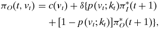 $$\begin{eqnarray}
\pi _O(t, v_t) &=& c(v_t) + \delta \lbrace p(v_t; k_t) \pi _I^{*}(t+1) \nonumber\\
&&+\, [1 - p(v_t; k_t)] \pi _O^{*}(t+1)\rbrace ,
\end{eqnarray}$$
$$\begin{eqnarray}
\pi _O(t, v_t) &=& c(v_t) + \delta \lbrace p(v_t; k_t) \pi _I^{*}(t+1) \nonumber\\
&&+\, [1 - p(v_t; k_t)] \pi _O^{*}(t+1)\rbrace ,
\end{eqnarray}$$
 $$\begin{eqnarray}
v_t^{*} \in \arg \max_{\hspace*{-20pt}v_{t} \ge 0} \pi _O(t, v_t),
\end{eqnarray}$$
$$\begin{eqnarray}
v_t^{*} \in \arg \max_{\hspace*{-20pt}v_{t} \ge 0} \pi _O(t, v_t),
\end{eqnarray}$$
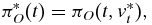 $$\begin{eqnarray}
\pi _O^{*}(t) = \pi _O(t, v_t^{*}),
\end{eqnarray}$$
$$\begin{eqnarray}
\pi _O^{*}(t) = \pi _O(t, v_t^{*}),
\end{eqnarray}$$
 $$\begin{eqnarray}
\pi _I^{*}(t) &=& \psi\, + \delta \{ p(v_t^{*}; k_t) \pi _O^{*}(t+1) \nonumber\\
&&+\, [1 - p(v_t^{*}; k_t)] \pi _I^{*}(t+1)\}.
\end{eqnarray}$$
$$\begin{eqnarray}
\pi _I^{*}(t) &=& \psi\, + \delta \{ p(v_t^{*}; k_t) \pi _O^{*}(t+1) \nonumber\\
&&+\, [1 - p(v_t^{*}; k_t)] \pi _I^{*}(t+1)\}.
\end{eqnarray}$$
An equilibrium to the model is characterized by sequences v* t , π* O (t), and π* I (t) that solve equations (2)–(5) for t = 1, . . ., T. It is also convenient to write the difference between the net present value of entering period t as the incumbent versus the as the opposition as Δ* t ≡ π* I (t) − π* O (t). So, the first order condition for an interior level of violence vt is
 $$\begin{eqnarray}
\delta \frac{\partial\, p(v_{t}; k_{t})}{\partial v_{t}} \Delta ^{*}_{t+1} = c^\prime (v_t).
\end{eqnarray}$$
$$\begin{eqnarray}
\delta \frac{\partial\, p(v_{t}; k_{t})}{\partial v_{t}} \Delta ^{*}_{t+1} = c^\prime (v_t).
\end{eqnarray}$$
As long as Δ* t + 1 > 0—which means it is better to enter the next period as the incumbent rather than as the opposition—this optimization problem has a unique interior solution v* t . If it is better to enter period t + 1 as the opposition rather than as the incumbent, there is no benefit to violence and hence it is optimal to pick v* t = 0.Footnote 14 So:
Proposition 1 The baseline model has a unique equilibrium where v* t solves equation (6) when Δ* t + 1 > 0 and v* t = 0 otherwise.
Proof. Follows from the above analysis; see the Appendix for details.
 $\Box$
Next we analyze how changing the effectiveness of violence in a given period affects the pattern of violence throughout the game. For simplicity we only consider the plausibly realistic case where it is better to enter as the incumbent in every period (i.e., when Δ* t > 0 for all t); see the Online Appendix for discussion of how loosening this restriction affects the results.
The direct effect of increasing the effectiveness of violence in period t is that by increasing the marginal effect of vt
on taking over office, the marginal benefit to violence increases, leading to a higher choice in period t. Formally, implicitly differentiating equation (6) gives that
 $\frac{\partial v_t^{*}}{\partial k_t} > 0$
.
$\frac{\partial v_t^{*}}{\partial k_t} > 0$
.
To formalize the indirect effect, consider how making violence more effective in future periods (i.e., t′ > t) affects behavior in period t. (By sequential rationality, violence levels in previous periods t′ < t do not affect the choice in period t.) Referring back to equation (6), this will depend on how the future effectiveness of violence changes the relative value of entering the next period as the incumbent (Δ* t + 1). When t′ = t + 1, the result is straightforward: making violence more effective in the next period unambiguously makes the opposition better off and the incumbent worse off entering this period. This reduces the relative value of entering the next period as the incumbent, so there is less violence in period t. For periods t′ > t + 1 the technical analysis is more subtle, but for all of the examples we present in our illustrations, reducing the effectiveness of violence at any future period decreases the level of violence today (see the Online Appendix for examples where this does not hold). Intuitively, as long as it is better to enter each period as the incumbent, and taking control of the government by force is rare, anything that makes doing so easier in the future reduces incentives to commit violence today. Formally:
Proposition 2 The equilibrium level of violence in time period t 1 is
(i) increasing in k t 1 ,
(ii) decreasing in k t 1 + 1, and
(iii) provided
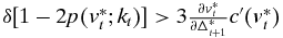 $\delta [1 - 2 p(v_t^{*}; k_t)] > 3\frac{\partial v_t^{*}}{\partial \Delta ^{*}_{t+1}} c^\prime (v_t^{*})$
for t ∈ {t
1, . . .t
2 − 1}, decreasing in k
t
2
for t
2 > t
1 + 1.
$\delta [1 - 2 p(v_t^{*}; k_t)] > 3\frac{\partial v_t^{*}}{\partial \Delta ^{*}_{t+1}} c^\prime (v_t^{*})$
for t ∈ {t
1, . . .t
2 − 1}, decreasing in k
t
2
for t
2 > t
1 + 1.
Proof. See the Appendix.
 $\Box$
While the model has not yet explicitly addressed elections, this result formalizes the central intuition about the direct and indirect effects of making violence more effective in a given period. The obvious direct effect is that there is more violence in this period. However, making violence more effective in period t has an indirect effect of decreasing violence in periods t − 1, and potentially in all periods prior to period t.
The idea that political actors time their actions is fairly well documented, especially in the terrorism literature. For instance, the Boston Marathon bombers had initially planned their attack for the July 4 festivities (Boston Reference Boston2013), and the so-called “underwear bomber” had timed his attack for Christmas Day (Hudson Reference Hudson2013). Such violent actors are also known to specifically wait for elections so that their attacks would have a greater impact. A recent prominent example of such an approach is the the 2004 train bombings in Madrid that took place three days before the Spanish voters went to the ballot, and is now known to have been timed specifically to influence the election outcome (Richburg Reference Richburg2004). Other similar instances include the Kurdistan Workers’ Party (PKK) attacking Turkish security forces to sway the electorate in April 2015 (Aksoy Reference Aksoy2015), and intelligence reports indicating that Pakistani terrorists planning suicide attacks timed for the Indian elections (Shukla Reference Shukla2014). Violence (including but not limited to terrorism) may also be more prevalent during seasons when it is easier to recruit fighters, for example because wages are lower outside of harvest seasons (Guardado and Pennings Reference Guardado and Pennings2015).Footnote 15
Proposition 2 indicates that this intuition can apply to the incentives to commit violence to gain political power. While some of these examples are from groups with no stated aspiration to actually take control of the government, in Section 4 we further argue that the logic applies to a wide class of political violence committed by various actors and various aims.
ELECTIONS IN THE BASELINE MODEL
With this general solution in place we now examine how periodic elections change aggregate levels of violence under the assumption that violence is more effective in electoral periods. For simplicity, we begin with a stark comparison between patterns of violence in a society with no elections versus one with periodic elections. We then turn to the question of how making elections more consequential and other more fine-grained changes affect patterns and aggregate levels of political violence.
A Simple Example
Suppose in a society without elections, the effectiveness of violence is kt = kn for all periods. In a society with elections, the effectiveness of violence is ke > kn in electoral periods and kn for other periods.
A simple microfoundation for this assumption is that the opposition can commit “nonelectoral” violence in any period, but electoral violence is only possible (or only useful) in electoral periods. So, in electoral periods, the opposition—and, as formalized in Section 4, other actors—have multiple ways to influence political outcomes with violence. While electoral violence can look much different than other forms of violence, for our purposes adding a new violent technology during elections is equivalent to assuming that violence is more effective in electoral periods (see the Online Appendix for a formal statement of this point). More broadly, we make this seemingly unusual assumption because our primary goal is to show how elections can reduce violence even if fighting peaks around elections. So this assumption constitutes a “hard case” for our aims.Footnote 16
As demonstrated by Proposition 2, introducing elections in this manner has a direct effect of increasing the level of violence in electoral periods but also an indirect effect of decreasing violence in the periods before elections, and potentially all nonelectoral periods. To show that either effect can be larger, we present several illustrative cases. For all of these examples, c(vt ) = v 2 t and p(vt ; kt ) = kt [1 − (1 + vt )−1].
Figure 3 presents a comparison of violence levels in two societies that only vary in the presence of elections. In both societies, there are 20 periods, and the effectiveness of violence in nonelectoral periods is kn = 0.3. Without elections (the grey line), all periods are nonelectoral, and the equilibrium violence choice is constant.Footnote 17 In the second society (black curve), there are elections in periods 6, 12, and 18 (the vertical lines), where the effectiveness of violence increases to ke = 1. The horizontal black line represents the average violence level with elections.

FIGURE 3. Comparison of Levels of Violence with No Elections (grey line) and Elections (black line)
The black curve presents a similar (if tidier) pattern as shown in the cases of Kenya and Ghana in Figure 1 with spikes in levels of violence in electoral periods (or years). While we cannot directly know what the counterfactual level of violence would be without elections using observational data, with the theoretical model we can make this comparison by looking at violence levels in an otherwise identical society with no elections. In this case, the black line is below the grey line, indicating that the spikes in electoral periods are more than offset by the decrease in violence in nonelectoral periods, leading to less fighting on average.Footnote 18 This example illustrates the first main result of the article in a simple fashion: the existence of a political violence cycle does not imply societies would become more peaceful without elections.Footnote 19
Next, we consider how general this example is by examining how changing various parameters of the model affects patterns and aggregate levels of violence. Unfortunately, analytic results on this relationship in the baseline model prove very difficult (stronger results along these lines emerge in the model with nonviolent actions in the next section). However, it is straightforward to simulate the model for a wide range of parameters and functional forms for the c and p functions to explore how this affects average levels of violence. The Online Appendix contains an extensive analysis of how changing individual parameters affects violence levels for randomly drawn values of the other parameters. In the main text, we focus on several results from this exercise that are of substantive interest and are generally robust to varying other parameters.
Consequential/Competitive Elections
First, Figure 4 shows a counterintuitive and empirically relevant example of how the degree to which violence is more effective during elections affects the average level of violence. The left panel illustrates the per period violence levels with increasingly dark lines as ke increases. Increasing the effectiveness of violence in the electoral periods leads to bigger spikes of violence during the election, but also larger decreases in violence in nonelectoral periods.

FIGURE 4. The Effect of Making Elections more Consequential on Average Levels of Violence
The right panel shows how this affects the average levels of violence (solid line) and the difference between the average level of violence in electoral periods versus nonelectoral periods (dotted line). While making violence slightly more effective in electoral periods increases the average amount of violence, making violence much more effective leads to less violence overall. However, increasing the effectiveness of violence unambiguously increases the difference between violence levels in electoral versus nonelectoral periods. So, for part of the parameter space, making electoral period violence more effective leads to bigger spikes of violence in electoral periods but less violence overall.
While this effect is just from one set of simulations (again, see the Online Appendix for an illustration of how this relationship changes for random draws of the other parameters) and the changes in the average violence level are not large, this illustration has important empirical and policy consequences. First, it is interesting in light of empirical findings that competitive elections outside of consolidated democracies tend to be particularly violent (Hafner-Burton, Hyde, and Jablonski Reference Hafner-Burton, Hyde, Ryan and Jablonski2014; Straus and Taylor Reference Straus and Taylor2012), as well as the sharper spike of violence in elections where the chief executive is at stake shown in Figure 2.
Elections with higher stakes can be directly interpreted as ones where ke is higher.Footnote 20 Connecting the competitiveness of elections to this parameter is less straightforward. However, when elections are close there can be a higher marginal return to any political activity that will lead to more votes, including violence.Footnote 21 So, in that sense, we might expect that competitive elections are ones where the marginal returns to violence are high, which is precisely what we mean by ke being high. Under this interpretation, it is the competitiveness of the election that depresses violence before the election: there is less of an incentive to commit violence today if the opposition has a real chance to take office in an upcoming election.
On the policy end, given that nearly every country holds some kind of election and few argue they should be abolished entirely, the comparison between more or less consequential elections is more relevant than the contrast between elections and no elections at all. Interestingly, this simulation suggests that to reap the benefits of elections in terms of peace it may not be enough to have elections that are only slightly consequential. Conversely, this example raises the possibility that making elections less consequential will lead to smaller spikes in violence during elections but also more violence overall.
Other Simulations
Figure 5 shows how changing several other parameters affects the difference in average levels of violence with and without elections. The left panel examines the effect of the discount rate. Changing δ has a nonmonotone effect. When the parties are extremely impatient (δ → 0) the optimal violence choice is always zero since the benefits of taking over office do not accrue right away. So if parties are completely impatient, there is no violence at all regardless of whether elections are held. For moderate levels of patience there can be more violence with elections, and the parties are patient enough to get a benefit from using violence but not patient enough for the prospect of future elections to outweigh the direct effect. When δ gets large, the indirect effect becomes stronger and elections lead to less violence overall.Footnote 22 For this particular parameterization, a discount rate of 0.88 is where elections go from promoting to preventing violence.

FIGURE 5. Comparative Statics on Change in Violence with Elections by the Discount Rate (left panel), Value of Office (middle panel), and Frequence of Elections (right panel)
The middle panel examines the value of holding office (ψ ). For this parameterization (and, as shown in the Online Appendix, the majority but not all of our simulations), increasing ψ always leads to elections having a more pacifying effect. A potential explanation for this is that there will be more violence in general when there are more spoils to fight over. When there is already a high level violence in the nonelectoral baseline, the marginal effect of making violence more effective in electoral periods is relatively low compared to potential to decrease violence by making it more effective in the future.
Finally, the right panel examines the frequency of elections. When elections are extremely frequent, they lead to more violence, as there is not enough time between elections for the indirect effect of making nonelectoral periods more peaceful to outweigh the direct effect. When elections are very rare, they lead to slightly less violence since it takes a long time to wait until the next election, weakening the indirect effect. So, the optimal election timing is intermediate, where nonelectoral periods are short enough that the indirect effect matters for the entire time between elections, but long enough that the indirect effect adds up to matter more than the direct effect.
EXTENSIONS
Several simplifying assumptions utilized so far raise doubts about the scope conditions for the model. First, by assuming that elections only increase the effectiveness of violence, we cannot yet say how providing nonviolent means to contest for power affects the patterns we describe. Second, much if not most political violence is perpetrated by the government and their agents, not just the opposition as in the baseline model. Third, so far we have only modeled violence committed to take over the government, while political violence often has other (and more incremental) goals. As our goal is to assess how elections affect broad patterns of political violence, it is important to check that similar results can come out of models with more realistic and general assumptions.
Fortunately, the results are robust and often even stronger when extending the model in several ways. In particular, we address these concerns with three modifications to the model that allow for nonviolent political technology, multiple actors committing violence, and violence to obtain goals other than taking over office. Doing so also provides more detailed empirical insights about when certain political actors are more or less apt to commit violence.
Bullets and Ballots
A central idea in the literature on democracy is that elections allow parties to compete for power with nonviolent means. Further, there are a number of empirical examples where armed groups have either delayed or renounced violence in the presence of nonviolent alternatives. For example, the Irish Republican Army (IRA) agreed to give up arms in Northern Ireland in 2005 when its political arm, Sinn Fein, made inroads in Northern Ireland and in the Irish Republic (Lavery and Cowell Reference Lavery and Cowell2005). Similarly, the Free Aceh Movement (GAM) in Indonesia give up violence as part of an agreement that included Indonesia allowing regional political parties to participate in national elections (Simanjuntak Reference Simanjuntak2008).
To combine our argument with the canonical claim that elections reduce violence by providing an alternative means to contest for power, we present an extension where the opposition can also use nonviolent actions. In short, we find that this leads to a substitution away from violence that can make society substantially more peaceful even though there is still a cycle of violence around elections.
To formalize this, suppose that in an electoral period, the opposition party can also choose to take nonviolent actions to increase their probability of becoming the incumbent following the election. Let xt represent the amount of nonviolent activity in period t, which could represent campaigning, mobilizing voters on election day, or other less desirable but nonviolent tactics like vote buying. Let the probability of taking office in an electoral period be p(xt + vt ; kt ) with the same functional form assumptions as above.Footnote 23 So, now the kt parameter reflects the increased effectiveness of political activity in general. To simplify the analysis, we assume that nonviolent political action is not available or ineffective in nonelectoral periods.
In addition to the cost c(vt ) paid to take violent actions, the opposition also pays a partial cost c(xt )/β t for the nonviolent actions, for some β t > 0. So, β t reflects the relative cost of violent political activity in period t: when β t > 1 violent activity is more efficient and when β t < 1 nonviolent action is more efficient.Footnote 24
Our solution concept (formalized in the Appendix) is analogous to the main model, except now the joint choice of violent and nonviolent action must be sequentially rational. Following standard optimization procedures, the first order condition for the opposition’s choice in period t is now the (vt, xt ) that jointly solve
 $$\begin{eqnarray}
\delta \frac{\partial\, p(x_t + v_t; k_t)}{\partial v_t} \Delta ^{*}_{t+1} = c^\prime (v_t),
\end{eqnarray}$$
$$\begin{eqnarray}
\delta \frac{\partial\, p(x_t + v_t; k_t)}{\partial v_t} \Delta ^{*}_{t+1} = c^\prime (v_t),
\end{eqnarray}$$
 $$\begin{eqnarray}
\delta \frac{\partial\, p(x_t + v_t; k_t)}{\partial x_t} \Delta ^{*}_{t+1} = c^\prime (x_t) / \beta_t ,
\end{eqnarray}$$
$$\begin{eqnarray}
\delta \frac{\partial\, p(x_t + v_t; k_t)}{\partial x_t} \Delta ^{*}_{t+1} = c^\prime (x_t) / \beta_t ,
\end{eqnarray}$$
where Δ* t + 1 is again the difference between the net present value of entering period t + 1 as the incumbent versus opposition. This implies c′(v* t ) = c′(xt *)/β t , which by the convexity of c ensures a unique pair (x* t , vt *) meeting these conditions. So, by an identical argument to the baseline model, there is a unique equilibrium level of violence and nonviolent activity (v* t , xt *) in each period characterized by Equations (7) and (8) when Δ* t > 0 and v* t = xt * = 0 when Δ* t ⩾ 0.
Figure 6 illustrates the impact of nonviolent activity on how much violence is chosen in equilibrium, with c(vt ) = −v 2 t and p(vt + xt ; kt ) = kt [1 − (1 + vt + xt )−1]. As before, the flat line in the left panel is the level of violence with no elections. The dotted curve represents the level of violence chosen where nonviolent technology is very expensive, and the spike in violence is large during the election is large relative to the dip in violence in no-electoral periods, resulting in more violence on average with elections despite some substitution to nonviolent activity.

FIGURE 6. The Effect of Introducing Nonviolent Technologies on the Level of Violence
In the solid curve, the nonviolent technology is cheaper (high β t , set to a constant β for all electoral periods), leading to a stronger substitution away from using violence during electoral periods. The availability of effective nonviolent technology also augments the intertemporal effects of the baseline model, as there is less reason to commit violence when it is possible to contest for power peacefully in future electoral periods. As a result, the level of violence is not only lower on average, but lower in every period than it would be without elections. The substitution effect is so large that violence peaks after the election, when (1) the nonviolent technology is not available, but (2) the next election is far enough away that it is worth committing violence to try and take over office. This pattern matches the case of Burkina Faso in Figure 1; we revisit the relationship between this example and several theoretical and empirical papers on postelection protest in the discussion. Still, the presence of elections induces a cyclical pattern of violence that, without thinking of the proper counterfactual, could erroneously lead to conclusions that elections encourage violence.
The right panel of Figure 6 plots the average level of violence as a function of the relative cost of violent actions (β). Unlike the previous graphs, making the nonviolent action cheaper (higher β) has an unambiguous and large effect in decreasing the average levels of violence. In this parameterization, elections would lead to more violence in the absence of a nonviolent technology (β → 0), but as long as the nonviolent technology is less than twice as expensive as violence the presence of elections will decrease the average level of violence.
Proposition 3 The model with non-violent technology has a unique equilibrium, where:
(i) the level of violence in electoral period t is decreasing in the relative cheapness of nonviolent technology (β t ), and
(ii) when the nonviolent technology becomes extremely cheap in period t, the level of violence approaches zero (as β t → ∞, v* t → 0).
Proof. See the Appendix.
 $\Box$
In other words, with substitution to non-violent technology the direct effect in the baseline model is weakened if not reversed, potentially leading to less violence in electoral periods. The logic of the indirect effect of reducing violence in non-electoral periods remains, and so elections can unambiguously reduce violence on average and even in every period (as in Figure 6).
Incumbent and Opposition Violence
Next, we analyze a case where both the incumbent and opposition can commit violence. In this section, we assume the probability that the opposition becomes the incumbent in period t + 1 as a function of their violence choice (now v O, t ⩾ 0) and the incumbent violence choice (v I, t ⩾ 0) is
 $$\begin{eqnarray*}
p(v_{O,t}, v_{I, t}; k_t) = \left\lbrace \begin{array}{@{}l@{\quad }l@{}}k_t \frac{v_{O,t}}{v_{O,t} + v_{I,t}} & v_{O,t} + v_{I,t} > 0\\
p_0 & v_{O,t} + v_{I,t} = 0 \end{array}\right.
\end{eqnarray*}$$
$$\begin{eqnarray*}
p(v_{O,t}, v_{I, t}; k_t) = \left\lbrace \begin{array}{@{}l@{\quad }l@{}}k_t \frac{v_{O,t}}{v_{O,t} + v_{I,t}} & v_{O,t} + v_{I,t} > 0\\
p_0 & v_{O,t} + v_{I,t} = 0 \end{array}\right.
\end{eqnarray*}$$
for some kt ∈ [0, 1] and p 0 ∈ (0, 1). (The v O, t + v I, t = 0 case is to avoid division by zero, and the exact value of p 0 has no impact on the analysis.) This functional form meets all of the assumptions with respect to v O, t and kt in the baseline model as long as v I, t > 0 (which will always be true in equilibrium).
Let the opposition cost for committing violence level v O, t be exactly v O, t , and let the cost of committing violence for the incumbent be γv I, t for some 0 < γ < 1. That is, we assume that violence is “cheaper” for the incumbent, or, equivalently, the incumbent gets a higher return to violence.Footnote 25
The rents for being the incumbent are again ψ. So, actor J’s net present value of committing violence level v J, t in period t (given the future violence choices) is
 $$\begin{eqnarray*}
\pi _O(t, v_{O,t}; v_{I, t}) &=& -v_{O,t} + \delta [p(v_{O,t}, v_{I,t}; k_t) \pi _I^{*}(t+1)\\
&&+\, [1 - p(v_{O,t}, v_{I, t}; k_t)] \pi _O^{*}(t+1)],\\
\pi _I(t, v_{O,t}; v_{I, t}) &=& \psi\; - \gamma v_{I,t} + \delta [p(v_{O,t}, v_{I,t}; k_t) \pi _O^{*}(t+1)\\
&&+\, [1 - p(v_{O,t}, v_{I, t}; k_t)] \pi _I^{*}(t+1)].
\end{eqnarray*}$$
$$\begin{eqnarray*}
\pi _O(t, v_{O,t}; v_{I, t}) &=& -v_{O,t} + \delta [p(v_{O,t}, v_{I,t}; k_t) \pi _I^{*}(t+1)\\
&&+\, [1 - p(v_{O,t}, v_{I, t}; k_t)] \pi _O^{*}(t+1)],\\
\pi _I(t, v_{O,t}; v_{I, t}) &=& \psi\; - \gamma v_{I,t} + \delta [p(v_{O,t}, v_{I,t}; k_t) \pi _O^{*}(t+1)\\
&&+\, [1 - p(v_{O,t}, v_{I, t}; k_t)] \pi _I^{*}(t+1)].
\end{eqnarray*}$$
Our solution concept now requires that the violence choices are mutual best responses given future violence choices (see the Appendix for a formal statement) By a standard analysis, whenever π* I (t + 1) > π O *(t + 1) the equilibrium violence choices are given by:
 $$\begin{eqnarray}
v_{O,t}^{*} = \frac{k_t \delta [\pi _I^{*}(t+1) - \pi _O^{*}(t+1)]}{(1 + \gamma ^{-1})^2},
\end{eqnarray}$$
$$\begin{eqnarray}
v_{O,t}^{*} = \frac{k_t \delta [\pi _I^{*}(t+1) - \pi _O^{*}(t+1)]}{(1 + \gamma ^{-1})^2},
\end{eqnarray}$$
 $$\begin{eqnarray}
v_{I,t}^{*} = \frac{\gamma ^{-1} k_t \delta [\pi _I^{*}(t+1) - \pi _O^{*}(t+1)]}{(1 + \gamma ^{-1})^2}
\end{eqnarray}$$
$$\begin{eqnarray}
v_{I,t}^{*} = \frac{\gamma ^{-1} k_t \delta [\pi _I^{*}(t+1) - \pi _O^{*}(t+1)]}{(1 + \gamma ^{-1})^2}
\end{eqnarray}$$
and if π* I (t + 1) < π O *(t + 1) both actors choose no violence (see the Appendix for detail). Since π* I (T + 1) > π O *(T + 1), the level of violence chosen in the last period is positive for both actors: v* J, T > 0.
It immediately follows from equations (9) and (10) that the level of violence chosen by both actors in period t (when strictly positive) is increasing in the effectiveness in period t. Further, since γ < 1, the incumbent always chooses more violence than the opposition, and hence always remains the incumbent with a probability greater than 1/2. As γ → 0, the incumbent commits far more violence than the opposition, indicating this extension can capture cases where the vast majority is committed by government forces.
Using these violence levels to compute the net present value for entering period t as each party, the difference between these payoffs is
 $$\begin{eqnarray}
\Delta ^{*}_t = \pi _I^{*}(t) - \pi _O^{*}(t) = \psi\, + \delta \left(1 - 2 \frac{k_t}{1 + \gamma ^{-1}}\right) \Delta ^{*}_{t+1}. \nonumber\\
\end{eqnarray}$$
$$\begin{eqnarray}
\Delta ^{*}_t = \pi _I^{*}(t) - \pi _O^{*}(t) = \psi\, + \delta \left(1 - 2 \frac{k_t}{1 + \gamma ^{-1}}\right) \Delta ^{*}_{t+1}. \nonumber\\
\end{eqnarray}$$
Since γ < 1, whenever Δ* t + 1 is positive, Δ* t is positive as well, so by induction Δ* t is positive for all t and hence both actors choose a strictly positive level of violence in each period. Further, Δ* t is decreasing in kt : when violence is more effective in period t, the difference between entering this period as the incumbent versus opposition decreases. So, there will be less violence committed in period t − 1 as kt increases.
The same inductive argument then implies that Δ* t − 1 is decreasing in kt , as is Δ* t′ for any t′ < t, and hence v* J, t − 1 is decreasing in kt for both J = I and J = O. Combined with the fact that the violence levels in period t are increasing in kt :
Proposition 4 In the two actor model, the level of violence committed by both actors in period t is increasing kt and decreasing in k t′ for all t′ < t.
Proof. See the Appendix.
 $\Box$
The intuition for the opposition violence choice is similar to the main model: if violence will be more effective in the future (e.g., because of an election), the opposition invests less in violence anticipating it will be more effective later. The fact that violence will be more effective in the future also leads the incumbent to choose less, as even if they are ousted they will have an opportunity to take power back during the election.
Another intuition for the incumbent violence choice is that they are reacting to anticipated violence choices by the opposition, and increasing the violence choice by the opposition gives the incumbent an incentive to commit more violence to counteract this. Formally, the marginal benefit for the incumbent violence choice is increasing in v O, t as long as v O, t < v I, t , which is always true in equilibrium. That is, making violence more effective for the opposition during elections can lead to more incumbent violence. During elections, this can lead to a spiral effect where the incumbent reacts to opposition violence with even more of their own. However, there is a similar but peaceful spiral effect in nonelectoral periods: since the opposition would rather wait to use violence, the government has less reason to repress them.
Continuous Policy Outcomes
Finally, a drawback of the models so far is that they only consider violence committed to take control of the government, while much political violence has more incremental goals. To show that the logic of our model applies to this more general class of political violence, we briefly present a variant of the model where a single political actor chooses a level of violence to affect a continuous policy outcome. Unlike before, there is only one actor and no “incumbency”; i.e., the same actor chooses a violence level in each period to influence the policy in their preferred direction.
Formally, the actor chooses violence level vt in each of T > 1 periods. The policy in period t + 1 is
 $$\begin{eqnarray*}
y_{t+1} = (1 - k_t) y_{t} + k_t v_t,
\end{eqnarray*}$$
$$\begin{eqnarray*}
y_{t+1} = (1 - k_t) y_{t} + k_t v_t,
\end{eqnarray*}$$
where kt ∈ [0, 1]. That is, the policy in each period is a weighted average of the past policy and the efforts of the political actor. When kt is higher, violence will be more effective in period t, or, equivalently, the status quo is “less sticky.” The period utility as a function of the policy and violence choice is
 $$\begin{eqnarray*}
u_t = y_t - c v_t^2
\end{eqnarray*}$$
$$\begin{eqnarray*}
u_t = y_t - c v_t^2
\end{eqnarray*}$$
and the payoff for the entire game is
 $$\begin{eqnarray*}
\sum _{i=1}^T \delta ^{i-1} u_i + a \delta ^T y_{T+1},
\end{eqnarray*}$$
$$\begin{eqnarray*}
\sum _{i=1}^T \delta ^{i-1} u_i + a \delta ^T y_{T+1},
\end{eqnarray*}$$
where a > 0 represents the relative importance of the policy at the end of the game.
The main insight from this model is that violence committed in period t increases the policy in every future period. However, the impact on periods beyond the next one is diminished by the fact that future policies are also shaped by future violence choices. In particular, a marginal increase in violence in period t increases y t + 1 by kt, y t + 2 by kt (1 − k t + 1), and for any τ > t + 1, y τ by kt ∏τ − 1 i = t + 1(1 − ki ). So, the total return to violence today is increasing in kt and decreasing in the effectiveness of violence in every future period:
Proposition 5 In the continuous policy model, the amount of violence committed in period t is
(i) increasing in kt ,
(ii) decreasing in k t′ for all t′ > t.
In addition to demonstrating that the results in the baseline model extend to “policies” other than who controls the government, this model provides an alternative intuition for why elections may reduce violence overall. When committing violence today, political actors are not just attempting to change the status quo for the “next period,” whether that be a day, year, or electoral cycle. Since policy tends to be sticky, the marginal benefit to violence today is a discounted sum of how violence today affects policy for every future period. The effective discount rate for the future is not just a function of patience, but whether whatever political gains made today could be reversed in the future. So, if elections increase the chance that any political gains may be reversed, there is less reason to commit violence in nonelectoral periods.
DISCUSSION
The central conclusion from all of the models is that comparisons between levels of violence in electoral versus nonelectoral periods using observational data can lead to misleading conclusions about the efficacy of elections for reducing the overall amount of violence in society. Put another way, that elections are violent is theoretically consistent with the general result that societies with more meaningful elections generally have lower levels of conflict (Cheibub and Hays Reference Cheibub and Hays2016, Gleditsch and Ruggeri Reference Gleditsch and Ruggeri2010; Hegre et al. Reference Hegre, Ellingsen, Gates and Gleditsch2001; Poe and Tate Reference Poe and Tate1994).
More specifically, the models also provide insight into several recent empirical studies of when certain types of elections in certain contexts are particularly violent. First, several recent studies examine the prevalence of postelection protests (Daxecker Reference Daxecker2012; Hyde and Marinov Reference Hyde and Marinov2014; Rozenas Reference Rozenas2012), and Straus and Taylor (Reference Straus and Taylor2012) find that in Africa most violence is perpetrated by regimes, but the relative share of violence perpetrated by opposition groups is higher after elections. Figure 7 shows this differential pattern from the SCAD data used before for progovernment and antigovernment violence. While progovernment violence tends to be higher leading up to and during election day, antigovernment violence is highest just after the election. (Of course the regime may respond to these protests with violence of their own; see e.g., Arriola Reference Arriola2014).

FIGURE 7. Patterns of Pro- and Antigovernment Violence Around Elections
Most theorizing about postelection protest is backward looking, in the sense that groups are motivated to protest the process or outcome of the election (Daxecker Reference Daxecker2012; Hyde and Marinov Reference Hyde and Marinov2014; Rozenas Reference Rozenas2012). This idea can be incorporated in our model by interpreting the time immediately after the voting as part of the electoral period, and postelection protest contributing to violence being more effective in electoral periods.
Our approach also highlights a more nuanced and forward-looking explanation for why opposition groups turn to violence after elections. Violence is particularly attractive to electoral losers in times just after defeat for several reasons. First, if parties are more apt to use violence when the status quo is unfavorable, parties losing elections will have more to gain by turning to violence. Second, as demonstrated in the extension with substitution, violence can peak after elections because this is a time when nonviolent political activity is relatively ineffective (compared to electoral periods) and it is the time when the opposition has the longest to wait until nonviolent technologies become available (and violent actions more effective) at the next election. That is, when a party has to wait a long time to affect policy via elections they are more apt to turn to violence to affect the status quo in the short term.
Our argument also provides insight into studies about what institutional contexts are most prone to spikes of violence around elections. Aksoy (Reference Aksoy2014) finds that terrorism in democracies tends to cluster around elections in systems with lower “electoral permissiveness,” meaning it is harder for small parties to have a formal role in politics. This can be interpreted in light of the model with violent and nonviolent technology. If low electoral permissiveness means that nonviolent technologies are not effective, marginalized groups resort to violence during the election as that is their only choice and the most effective time to do so.
What does our model have to say in terms of novel predictions for future empirical work? We view the generality and small number of parameters in the model as a feature which provides confidence that the core of our argument holds across many political settings. However, this also means there are few comparative static predictions about how different institutions or other political and economic variables affect how much violence will be used during elections or the difference between violence levels in electoral versus nonelectoral periods. So, one way to push the literature forward both theoretically and then empirically would be to write models that combine the forces we introduce here with political institutions to generate comparative static predictions on variables which we could map to data.
Perhaps more importantly, future empirical work could aim to examine our more general contention that the ability to attain political goals during elections, whether with violence (parts (ii) and (iii) of Proposition 2) or other nonviolent tactics (part (i) of Proposition 3) makes politics more peaceful in nonelectoral periods. Isolating variables that only change the effectiveness in electoral periods (but not elsewhere) could prove difficult. One potential avenue for doing so would be to examine how (preferably exogenous) changes to expectations about how competitive future elections will be affect violence in time periods after this revelation but before the election. Another potential empirical avenue would be to examine the effect of elections in places that hold both scheduled and early elections, and analyze whether it leads to a political violence cycle similar to the available evidence on budget cycles (Khemani Reference Khemani2004).
CONCLUSION
Elections play an important role in democracies but they are often accompanied by violence against both candidates and voters. We have shown that the spike in conflict levels around elections does not necessarily imply that elections cause more political violence in general. When elections are the central means to contest for political power, they may also become the most effective times to use political violence. It is precisely the expectation of the ability to use violence effectively in a future electoral period that results in relatively lower levels of violence in nonelectoral periods. When elections also provide a nonviolent means to contest for power, there is even less reason to commit violence both during electoral and nonelectoral periods. Elections can be peaceful for two reasons: either they are not a serious means to contest for power, or they provide such an effective nonviolent means to contest for power that violence is no longer a useful tool.
More generally, the model highlights cycles of any political activity surrounding elections, whether fiscal policy, repression, or interest group attempts to influence policy do not mean these activities would be more or less prevalent if elections were less consequential. When the actions spiking around elections are “bad” it is easy to associate elections with negative consequences, but concentrating the time window in which these bad actions are most effective may leave citizens better off in the long term. So, empirical work examining how elections affect patterns of any political activity must keep in mind the effects of intertemporal substitution when thinking through the broader implications of their findings.
APPENDIX
Data
Figure 8 shows how the patterns we identify are less stark but still clear when looking at wider time windows around elections.

FIGURE 8. Violence Around Elections for Wider Time Windows
For this and the graphs in the main text, we use two main data sources to examine the empirical patterns of violence around elections. Violence data are obtained from the Social Conflict Analysis Database (SCAD), Version 3.0 (Hendrix and Salehyan Reference Salehyan, Hendrix, Hamner, Case, Linebarger, Stull and Williams2012). This dataset provides information on different types of violent events (protests, riots, strikes, and other social disturbances) in Africa and Latin America from 1990 to 2012. The main source of these events are based on the Associated Press and Agence France Presse news wires, indexed by the Lexis-Nexis news service.Footnote 26 Election dates and characteristics are from the National Elections Across Democracy and Autocracy (NELDA) Dataset (Hyde and Marinov Reference Hyde and Marinov2012). This dataset provides information on election events for all countries during the period 1945–2010.Footnote 27
To generate these figures, we first reshape the SCAD data into a “country-day” unit of analysis. Second, for each country and each day we determined the distance to the nearest election using the NELDA data. For example, if the previous election in a country was 200 days ago and the next is in 201 days, the distance to election variable is − 200. In the next day when the previous election was 201 days ago and the next is in 200 days, the distance variable becomes 200. Figures 2, 7, and 8 plot the average levels of violence levels by this distance to election variable, sometimes for subsets of the data identified by other characteristics.
For Figure 2, we distinguish between elections when the incumbent leader’s office was in contention versus when it was not. This was done using the variable in the NELDA dataset that captured whether the office of the incumbent leader was contested in a given election.
For Figure 7, distinguished between pro- and antigovernment violence around elections, progovernment violence was identified using the variable in the SCAD dataset that captures “distinct violent events waged primarily by government authorities, or by groups acting in explicit support of government authority, targeting individual, or ‘collective individual,’ members of an alleged opposition group or movement.” Antigovernment violence was identified using whether the “central government the target of the event,” and whether any of the issue areas involved elections.Footnote 28
Proof of Proposition 1
Equation (3) has a unique solution for t = T, which gives unique values of π*
O
(T) and π*
I
(T), which then implies the optimal v*
T − 1 by equation (6). Further, if there is a unique π*
O
(t) and π*
I
(t), this leads to a unique v*
t − 1, which is given by equation (6) when Δ*
t
⩽ 0 and equal to zero otherwise. So, by induction there is a unique triple of sequences (π*
I
(t), π
O
*(t), v*
t
) which solve equations (2)–(5) for all t.
 $\Box$
Proof of Proposition 2
Figure 9 illustrates the logic of how how changing kt affects the violence choices and relative value of incumbency for periods up to t.
FIGURE 9. Illustration of Proposition 2
The most direct effect of increasing kt is to increase the level of violence in period t, which can be demonstrated by implicitly differentiating equation (6) with respect to kt :
 $$\begin{eqnarray*}
\frac{\partial v_t^{*}}{\partial k_t} = \frac{- \frac{\partial ^2 p(v_{t}; k_{t})}{\partial v_{t} \partial k_t} \Delta ^{*}_{t+1}}{\frac{\partial ^2 p(v_{t}; k_{t})}{\partial ^2 v_{t}} \Delta ^{*}_{t+1} - c^{\prime \prime }(v_t^{*})} > 0,
\end{eqnarray*}$$
$$\begin{eqnarray*}
\frac{\partial v_t^{*}}{\partial k_t} = \frac{- \frac{\partial ^2 p(v_{t}; k_{t})}{\partial v_{t} \partial k_t} \Delta ^{*}_{t+1}}{\frac{\partial ^2 p(v_{t}; k_{t})}{\partial ^2 v_{t}} \Delta ^{*}_{t+1} - c^{\prime \prime }(v_t^{*})} > 0,
\end{eqnarray*}$$
where the inequality is true because the numerator is negative and the denominator is negative at v* t since it is at a local maximum.
The effect of increasing kt on v* t − 1 is determined by how increasing kt affects Δ* t , which in turn affects v* t − 1. Formally,
 $$\begin{eqnarray*}
\frac{\partial \Delta ^{*}_t}{k_t} = \frac{\partial \pi _I^{*}(t)}{k_t} - \frac{\partial \pi _O^{*}(t)}{k_t}.
\end{eqnarray*}$$
$$\begin{eqnarray*}
\frac{\partial \Delta ^{*}_t}{k_t} = \frac{\partial \pi _I^{*}(t)}{k_t} - \frac{\partial \pi _O^{*}(t)}{k_t}.
\end{eqnarray*}$$
The effect of increasing kt on π* I (t) is entirely through the fact that doing so increases p(v* t ; kt ), both directly by increasing kt and indirectly by increasing v* t . So
 $$\begin{eqnarray*}
\frac{\partial \pi _I^{*}(t)}{\partial k_t} = - \delta \Delta ^{*}_{t+1} \frac{d\, p(v_t^{*}; k_t)}{d k_t} < 0.
\end{eqnarray*}$$
$$\begin{eqnarray*}
\frac{\partial \pi _I^{*}(t)}{\partial k_t} = - \delta \Delta ^{*}_{t+1} \frac{d\, p(v_t^{*}; k_t)}{d k_t} < 0.
\end{eqnarray*}$$
For the change in the value of entering as the opposition the analogous calculation has more terms as they incur a higher cost to commit more violence, but by the envelope theorem this effect drops out, giving
 $$\begin{eqnarray*}
\frac{\partial \pi _O^{*}(t)}{\partial k_t} &=& -\frac{\partial v_t^{*}}{\partial k_t} c^\prime (v_t^{*}) + \delta \Delta ^{*}_{t+1} \frac{d\, p(v_t^{*}; k_t)}{d k_t}\\
&=& -\frac{\partial v_t^{*}}{\partial k_t} \left(-c^\prime (v_t^{*}) + \delta \Delta ^{*}_{t+1} \frac{\partial\, p(v_t^{*}; k_t)}{\partial v_t^{*}} \right)\\
&& +\, \delta \Delta ^{*}_{t+1} \frac{\partial\, p(v_t^{*}; k_t)}{\partial k_t}\\
&=& \delta \Delta ^{*}_{t+1} \frac{\partial\, p(v_t^{*}; k_t)}{\partial k_t} > 0.
\end{eqnarray*}$$
$$\begin{eqnarray*}
\frac{\partial \pi _O^{*}(t)}{\partial k_t} &=& -\frac{\partial v_t^{*}}{\partial k_t} c^\prime (v_t^{*}) + \delta \Delta ^{*}_{t+1} \frac{d\, p(v_t^{*}; k_t)}{d k_t}\\
&=& -\frac{\partial v_t^{*}}{\partial k_t} \left(-c^\prime (v_t^{*}) + \delta \Delta ^{*}_{t+1} \frac{\partial\, p(v_t^{*}; k_t)}{\partial v_t^{*}} \right)\\
&& +\, \delta \Delta ^{*}_{t+1} \frac{\partial\, p(v_t^{*}; k_t)}{\partial k_t}\\
&=& \delta \Delta ^{*}_{t+1} \frac{\partial\, p(v_t^{*}; k_t)}{\partial k_t} > 0.
\end{eqnarray*}$$
Since
 $\frac{\partial \pi _O^{*}(t)}{\partial k_t} > 0$
and
$\frac{\partial \pi _O^{*}(t)}{\partial k_t} > 0$
and
 $\frac{\partial \pi _I^{*}(t)}{\partial k_t} < 0$
,
$\frac{\partial \pi _I^{*}(t)}{\partial k_t} < 0$
,
 $\frac{\partial \Delta ^{*}_t}{k_t} < 0$
. Since there is less benefit to entering period t as the incumbent, this decreases the incentives to commit violence in period t − 1:
$\frac{\partial \Delta ^{*}_t}{k_t} < 0$
. Since there is less benefit to entering period t as the incumbent, this decreases the incentives to commit violence in period t − 1:
 $$\begin{eqnarray*}
\frac{\partial v_{t-1}^{*}}{\partial k_t} = - \frac{\frac{\partial\, p(v_{t}; k_{t})}{\partial v_{t}} \frac{\partial \Delta ^{*}_t}{\partial k_t}}{\frac{\partial ^2 p(v_{t}; k_{t})}{\partial ^2 v_{t}} \Delta ^{*}_{t+1} - c^{\prime \prime }(v_t)} < 0.
\end{eqnarray*}$$
$$\begin{eqnarray*}
\frac{\partial v_{t-1}^{*}}{\partial k_t} = - \frac{\frac{\partial\, p(v_{t}; k_{t})}{\partial v_{t}} \frac{\partial \Delta ^{*}_t}{\partial k_t}}{\frac{\partial ^2 p(v_{t}; k_{t})}{\partial ^2 v_{t}} \Delta ^{*}_{t+1} - c^{\prime \prime }(v_t)} < 0.
\end{eqnarray*}$$
The effect on even earlier periods is more nuanced. As shown in Figure 9, how kt affects violence in t′ < t − 1, depends on how kt affects Δ* t′, which in turn depends on how kt affects Δ* t′ + 1. This is given by
 $$\begin{eqnarray*}
\frac{\partial v_{t^\prime }^{*}}{\partial k_t} = - \frac{\frac{\partial\, p(v_{t^\prime }; k_{t^\prime })}{\partial v_{t^\prime }} \frac{\partial \Delta ^{*}_{t^\prime + 1}}{\partial k_t}}{\frac{\partial ^2 p(v_{t}; k_{t})}{\partial ^2 v_{t}} \Delta ^{*}_{t^\prime +1} - c^{\prime \prime }(v_t)},
\end{eqnarray*}$$
$$\begin{eqnarray*}
\frac{\partial v_{t^\prime }^{*}}{\partial k_t} = - \frac{\frac{\partial\, p(v_{t^\prime }; k_{t^\prime })}{\partial v_{t^\prime }} \frac{\partial \Delta ^{*}_{t^\prime + 1}}{\partial k_t}}{\frac{\partial ^2 p(v_{t}; k_{t})}{\partial ^2 v_{t}} \Delta ^{*}_{t^\prime +1} - c^{\prime \prime }(v_t)},
\end{eqnarray*}$$
which has the same sign as
 $\frac{\partial \Delta ^{*}_{t^\prime + 1}}{\partial k_t}$
. To sign this, first write Δ*
t
as
$\frac{\partial \Delta ^{*}_{t^\prime + 1}}{\partial k_t}$
. To sign this, first write Δ*
t
as
 $$\begin{eqnarray*}
\Delta ^{*}_t = \psi\, - c(v_t^{*}) + \delta [1 - 2 p(v_t^{*}; k_t)] \Delta ^{*}_{t+1}.
\end{eqnarray*}$$
$$\begin{eqnarray*}
\Delta ^{*}_t = \psi\, - c(v_t^{*}) + \delta [1 - 2 p(v_t^{*}; k_t)] \Delta ^{*}_{t+1}.
\end{eqnarray*}$$
So
 $$\begin{eqnarray}
\nonumber \frac{\partial \Delta ^{*}_t}{\partial \Delta ^{*}_{t+1}} &=& -\frac{\partial v_t^{*}}{\partial \Delta ^{*}_{t+1}} c^\prime (v_t^{*}) \nonumber\\
&&+\, \delta \left([1 - 2 p(v_t^{*}; k_t)] - 2 \Delta ^{*}_{t+1} \frac{\partial\, p(v_t^{*}; k_t)}{\partial v_t^{*}} \frac{\partial v_t^{*}}{\partial \Delta ^{*}_{t+1}} \right) \nonumber\\
&=& \frac{\partial v_t^{*}}{\partial \Delta ^{*}_{t+1}} \left(-c^\prime (v_t^{*}) - 2 \Delta ^{*}_{t+1} \frac{\partial\, p(v_t^{*}; k_t)}{\partial v_t^{*}} \right)\nonumber\\
&&+\, \delta [1 - 2 p(v_t^{*}; k_t)] \nonumber\\
&=& - 3\frac{\partial v_t^{*}}{\partial \Delta ^{*}_{t+1}} c^\prime (v_t^{*}) + \delta [1 - 2 p(v_t^{*}; k_t)],
\end{eqnarray}$$
$$\begin{eqnarray}
\nonumber \frac{\partial \Delta ^{*}_t}{\partial \Delta ^{*}_{t+1}} &=& -\frac{\partial v_t^{*}}{\partial \Delta ^{*}_{t+1}} c^\prime (v_t^{*}) \nonumber\\
&&+\, \delta \left([1 - 2 p(v_t^{*}; k_t)] - 2 \Delta ^{*}_{t+1} \frac{\partial\, p(v_t^{*}; k_t)}{\partial v_t^{*}} \frac{\partial v_t^{*}}{\partial \Delta ^{*}_{t+1}} \right) \nonumber\\
&=& \frac{\partial v_t^{*}}{\partial \Delta ^{*}_{t+1}} \left(-c^\prime (v_t^{*}) - 2 \Delta ^{*}_{t+1} \frac{\partial\, p(v_t^{*}; k_t)}{\partial v_t^{*}} \right)\nonumber\\
&&+\, \delta [1 - 2 p(v_t^{*}; k_t)] \nonumber\\
&=& - 3\frac{\partial v_t^{*}}{\partial \Delta ^{*}_{t+1}} c^\prime (v_t^{*}) + \delta [1 - 2 p(v_t^{*}; k_t)],
\end{eqnarray}$$
where the last line follows from the period t equilibrium condition (equation (6)). Rearranging,
 $\frac{\partial \Delta ^{*}_t}{\partial \Delta ^{*}_{t+1}} > 0$
if and only if
$\frac{\partial \Delta ^{*}_t}{\partial \Delta ^{*}_{t+1}} > 0$
if and only if
 $$\begin{eqnarray}
\delta [1 - 2 p(v_t^{*}; k_t)] > 3\frac{\partial v_t^{*}}{\partial \Delta ^{*}_{t+1}} c^\prime (v_t^{*}).
\end{eqnarray}$$
$$\begin{eqnarray}
\delta [1 - 2 p(v_t^{*}; k_t)] > 3\frac{\partial v_t^{*}}{\partial \Delta ^{*}_{t+1}} c^\prime (v_t^{*}).
\end{eqnarray}$$
From part (ii) we know that
 $\frac{\partial \Delta ^{*}_t}{\partial k_t} < 0$
, and if equation (13) holds for all t′, . . ., t − 1, then
$\frac{\partial \Delta ^{*}_t}{\partial k_t} < 0$
, and if equation (13) holds for all t′, . . ., t − 1, then
 $\frac{\partial \Delta ^{*}_{t-1}}{\partial \Delta ^{*}_t} > 0$
for each of these periods, and hence by induction
$\frac{\partial \Delta ^{*}_{t-1}}{\partial \Delta ^{*}_t} > 0$
for each of these periods, and hence by induction
 $\frac{\partial v_{t^\prime }^{*}}{\partial k_t} < 0$
.
$\frac{\partial v_{t^\prime }^{*}}{\partial k_t} < 0$
.
Equilibrium Definition for Extension with Nonviolent Action
An equilibrium to the model with nonviolent action is a x* t , v* t , π* O (t), and π* I (t) that solve
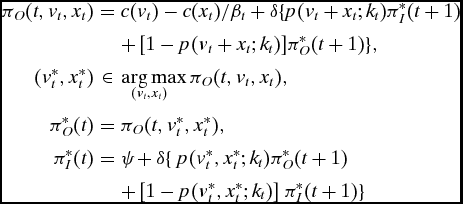 $$\begin{eqnarray*}
\pi _O(t, v_t, x_t) &=& c(v_t) - c(x_t)/\beta_t + \delta \lbrace p(v_t+ x_t; k_t) \pi _I^{*}(t+1)\\
&&+\,[1 - p(v_t + x_t; k_t)] \pi _O^{*}(t+1)\rbrace ,\\
(v_t^{*}, x_t^{*}) &\in & \arg \max _{\hspace*{-20pt}(v_t, x_t)} \pi _O(t, v_t, x_t),\\
\pi _O^{*}(t) &=& \pi _O(t, v_t^{*}, x_t^{*}),\\
\pi _I^{*}(t) &=& \psi\; + \delta \lbrace \ p(v_t^{*}, x_t^{*}; k_t) \pi _O^{*}(t+1) \\
&&+\, [1 - p(v_t^{*}, x_t^{*}; k_t)] \ \pi _I^{*}(t+1)\rbrace
\end{eqnarray*}$$
$$\begin{eqnarray*}
\pi _O(t, v_t, x_t) &=& c(v_t) - c(x_t)/\beta_t + \delta \lbrace p(v_t+ x_t; k_t) \pi _I^{*}(t+1)\\
&&+\,[1 - p(v_t + x_t; k_t)] \pi _O^{*}(t+1)\rbrace ,\\
(v_t^{*}, x_t^{*}) &\in & \arg \max _{\hspace*{-20pt}(v_t, x_t)} \pi _O(t, v_t, x_t),\\
\pi _O^{*}(t) &=& \pi _O(t, v_t^{*}, x_t^{*}),\\
\pi _I^{*}(t) &=& \psi\; + \delta \lbrace \ p(v_t^{*}, x_t^{*}; k_t) \pi _O^{*}(t+1) \\
&&+\, [1 - p(v_t^{*}, x_t^{*}; k_t)] \ \pi _I^{*}(t+1)\rbrace
\end{eqnarray*}$$
for t = 1, . . ., T. The main difference between this and the main model is that there are two optimizing choices v* t and x* t .
Proof of Proposition 3
The idea of the proof is to show that if the level of violence is nondecreasing in β t , then the opposition must use strictly more non-violent technology as β t increases, which lowers the marginal value of using violence, contradicting the violence choice being nondecreasing. Formally, consider any β1 > β2, and let (x 1 t , vt 1) and (x 2 t , vt 2) be the equilibrium decisions with these two values of beta. Suppose v 1 t ⩾ vt 2. Since c′ is increasing, this implies c′(v 1 t ) ⩾ c′(vt 2), and since c′(vi t ) = c′(xt i )/β i , c′(x 1 t )/β1 ⩾ c′(x 2 t )/β2. Combined with β1 > β2, this requires c′(x 1 t ) > c′(xt 2) and hence x 1 t > xt 2. But the equilibrium conditions for the violence choice for both levels of β t and the concavity of p( · ) imply that:
 $$\begin{eqnarray*}
c^\prime (v_t^1) = \frac{\partial\, p(x_t^1 + v_t^1; k_t)}{\partial x_t} \delta \Delta ^*_{t+1} < \frac{\partial \,p(x_t^2 + v_t^2; k_t)}{\partial x_t} \delta \Delta ^*_{t+1} = c^\prime (v_t^2)
\end{eqnarray*}$$
$$\begin{eqnarray*}
c^\prime (v_t^1) = \frac{\partial\, p(x_t^1 + v_t^1; k_t)}{\partial x_t} \delta \Delta ^*_{t+1} < \frac{\partial \,p(x_t^2 + v_t^2; k_t)}{\partial x_t} \delta \Delta ^*_{t+1} = c^\prime (v_t^2)
\end{eqnarray*}$$
which contradicts v 1 t ⩾ vt 2. So, vt must be strictly increasing in β t , proving part i.
For part ii, it follows from part i that c′(v*
t
) is decreasing in β
t
, so c′(x*
t
)/β
t
must be decreasing in β
t
as well. If this fraction approaches zero as β
t
→ ∞, then c′(v*
t
) → 0, which implies v*
t
→ 0. If c′(x*
t
)/β
t
does not go to zero as β
t
→ ∞, then it must be the case that x*
t
→ ∞, which implies
 $\frac{\partial\, p(x_t^* + v_t;\, k_t)}{\partial v_t} \rightarrow 0$
and hence v*
t
→ 0.
$\frac{\partial\, p(x_t^* + v_t;\, k_t)}{\partial v_t} \rightarrow 0$
and hence v*
t
→ 0.
Equilibrium Definition for Extension with Incumbent Violence
An equilibrium to the model with incumbent and opposition violence is a v* O, t , v* I, t , π* O (t), and π* I (t) that solve
 $$\begin{eqnarray*}
\pi _O(t, v_{I,t}, v_{O,t}) &=& c(v_{O,t}) + \delta \lbrace p(v_{I,t}, v_{O,t}; k_t) \pi _I^{*}(t+1)\\
&&+\, [1 - p(v_{I,t}, v_{O,t}; k_t)] \pi _O^{*}(t+1)\rbrace ,\\
\pi _I(t, v_{I,t}, v_{O,t}) &=& c(v_{I,t}) + \delta \lbrace p(v_{I,t}, v_{O,t}; k_t) \pi _O^{*}(t+1) \\
&&+\, [1 - p(v_{I,t}, v_{O,t}; k_t)] \pi _I^{*}(t+1)\rbrace ,\\
v_{I,t}^{*} &\in & \arg \max _{\hspace*{-20pt}v_{I,t}} \pi _I(t, v_{I,t},v_{O,t}^{*}),\\
v_{O,t}^{*} &\in & \arg \max _{\hspace*{-20pt}v_{O,t}} \pi _O(t, v_{I,t}^{*},v_{O,t}),\\
\pi _O^{*}(t) &=& \pi _O(t, v_{O,t}^{*}, v_{I,t}^{*}),\\
\pi _I^{*}(t) &=& \psi\, + \delta \lbrace p(v_{I,t}^{*}, v_{O,t}^{*}; k_t) \pi _O^{*}(t+1)\\
&&+\, [1 - p(v_{I,t}^{*}, v_{O,t}^{*}; k_t)] \pi _I^{*}(t+1)\rbrace
\end{eqnarray*}$$
$$\begin{eqnarray*}
\pi _O(t, v_{I,t}, v_{O,t}) &=& c(v_{O,t}) + \delta \lbrace p(v_{I,t}, v_{O,t}; k_t) \pi _I^{*}(t+1)\\
&&+\, [1 - p(v_{I,t}, v_{O,t}; k_t)] \pi _O^{*}(t+1)\rbrace ,\\
\pi _I(t, v_{I,t}, v_{O,t}) &=& c(v_{I,t}) + \delta \lbrace p(v_{I,t}, v_{O,t}; k_t) \pi _O^{*}(t+1) \\
&&+\, [1 - p(v_{I,t}, v_{O,t}; k_t)] \pi _I^{*}(t+1)\rbrace ,\\
v_{I,t}^{*} &\in & \arg \max _{\hspace*{-20pt}v_{I,t}} \pi _I(t, v_{I,t},v_{O,t}^{*}),\\
v_{O,t}^{*} &\in & \arg \max _{\hspace*{-20pt}v_{O,t}} \pi _O(t, v_{I,t}^{*},v_{O,t}),\\
\pi _O^{*}(t) &=& \pi _O(t, v_{O,t}^{*}, v_{I,t}^{*}),\\
\pi _I^{*}(t) &=& \psi\, + \delta \lbrace p(v_{I,t}^{*}, v_{O,t}^{*}; k_t) \pi _O^{*}(t+1)\\
&&+\, [1 - p(v_{I,t}^{*}, v_{O,t}^{*}; k_t)] \pi _I^{*}(t+1)\rbrace
\end{eqnarray*}$$
for t = 1, . . ., T. The main difference between this and the main model is that the incumbent and opposition choices must be mutual best responses, rather than the opposition violence choice being optimal in isolation.
Derivation of equations (9) and (10) and Proof of Proposition 4
The first order conditions if both actors choose a strictly positive level of violence are
 $$\begin{eqnarray*}
&& 1 = k_t \delta [\pi _I^{*}(t+1) - \pi _O^{*}(t+1)] \frac{v_{I,t}^{*}}{(v_{O,t} + v_{I, t}^{*})^2},\\
&& \gamma = k_t \delta [\pi _I^{*}(t+1) - \pi _O^{*}(t+1)]\frac{v_{O,t}^{*}}{(v_{O,t}^{*} + v_{I, t}^{*})^2}.
\end{eqnarray*}$$
$$\begin{eqnarray*}
&& 1 = k_t \delta [\pi _I^{*}(t+1) - \pi _O^{*}(t+1)] \frac{v_{I,t}^{*}}{(v_{O,t} + v_{I, t}^{*})^2},\\
&& \gamma = k_t \delta [\pi _I^{*}(t+1) - \pi _O^{*}(t+1)]\frac{v_{O,t}^{*}}{(v_{O,t}^{*} + v_{I, t}^{*})^2}.
\end{eqnarray*}$$
If π* I (t + 1) < π O *(t + 1) there can be no solution to these equations: the objective functions are always decreasing in v J, t , so in any equilibrium both actors choose v* J, t = 0.
If π*
I
(t + 1) > π
O
*(t + 1) and both actors chose no violence, there is an upward discontinuity in the probability of taking over office at v
J, t
= 0, so it is always better to choose an incrementally small level of violence to no violence. If only one actor chose a strictly positive level of violence, the other actor could always deviate to a lower violence level and have the same probability of being the incumbent in the next period. So, when π*
I
(t + 1) > π
O
*(t + 1) both violence levels must be interior, and by the preceding system of equation, this implies v*
I, t
= γ−1
v
O, t
*. Since violence is cheaper for the incumbent, they choose more in equilibrium. This also implies that in equilibrium the probability of a transition of power in each period is
 $\frac{k_t}{1 + \gamma ^{-1}}$
.
$\frac{k_t}{1 + \gamma ^{-1}}$
.
The net present values for entering in each role in period t when choosing the equilibrium level of violence is
 $$\begin{eqnarray}
\pi _O^{*}(t) &=& -v_{O,t}^{*} + \delta \Big[\frac{k_t}{1 + \gamma ^{-1}} \pi _I^{*}(t+1) \nonumber\\
&&+\, \left(1 - \frac{k_t}{1 + \gamma ^{-1}}\right) \pi _O^{*}(t+1)\Big],
\end{eqnarray}$$
$$\begin{eqnarray}
\pi _O^{*}(t) &=& -v_{O,t}^{*} + \delta \Big[\frac{k_t}{1 + \gamma ^{-1}} \pi _I^{*}(t+1) \nonumber\\
&&+\, \left(1 - \frac{k_t}{1 + \gamma ^{-1}}\right) \pi _O^{*}(t+1)\Big],
\end{eqnarray}$$
 $$\begin{eqnarray}
\pi _I^{*}(t) &=& \psi\, -\gamma v_{I,t}^{*} + \delta \Big[\frac{k_t}{1 + \gamma ^{-1}} \pi _O^{*}(t+1) \nonumber\\
&&+\, \left(1 - \frac{k_t}{1 + \gamma ^{-1}}\right) \pi _I^{*}(t+1)\Big]
\end{eqnarray}$$
$$\begin{eqnarray}
\pi _I^{*}(t) &=& \psi\, -\gamma v_{I,t}^{*} + \delta \Big[\frac{k_t}{1 + \gamma ^{-1}} \pi _O^{*}(t+1) \nonumber\\
&&+\, \left(1 - \frac{k_t}{1 + \gamma ^{-1}}\right) \pi _I^{*}(t+1)\Big]
\end{eqnarray}$$
and the formula for Δ* t follows from subtracting these.
For the proposition, part (i) follows immediately from equations (9) and (10). For part (ii), consider what happens when violence becomes more effective in some period t′. By equation (11), Δ*
t′ is decreasing in k′
t
, which then implies that v*
J, t′ − 1 and Δ*
t′ − 1 are both decreasing in k
t′. This in turn implies that v*
J, t′ − 2 and Δ*
t′ − 2 are decreasing in k
t′. More generally, v*
J, t′ − j
and Δ*
t′ − j
decreasing implies that v*
J, t′ − j − 1 and Δ*
t′ − j − 1 are decreasing. The result then follows by induction.
 $\Box$
Proof of Proposition 5
An equilibrium to the continuous policy outcome model is a sequence of violence choices where each v* t maximizes the expected payoff for the remainder of the game given the future violence choices.
So, in period T, the actor chooses vT to maximize
 $$\begin{eqnarray*}
y_{T} - \delta ^{T-1} c v_T^2 + a \delta ^T [(1 - k_T) y_T + k_T v_T],
\end{eqnarray*}$$
$$\begin{eqnarray*}
y_{T} - \delta ^{T-1} c v_T^2 + a \delta ^T [(1 - k_T) y_T + k_T v_T],
\end{eqnarray*}$$
giving first order condition,
 $$\begin{eqnarray*}
2c v_T = \delta a k_T,
\end{eqnarray*}$$
$$\begin{eqnarray*}
2c v_T = \delta a k_T,
\end{eqnarray*}$$
and hence v* T = δakT /2c.
In period T − 1, the actor picks v T − 1 to maximize
 $$\begin{eqnarray*}
&&\delta ^{T-2} c v_{T-1}^2 + \delta ^{T-1} [(1 - k_{T-1}) y_{T-1} + k_{T-1} v_{T-1}] \\
&&\quad +\, a \delta ^T \lbrace (1 - k_T)[(1 - k_{T-1}) y_{T-1} + k_{T-1} v_{T-1}] + k_T v_T^{*}\rbrace .
\end{eqnarray*}$$
$$\begin{eqnarray*}
&&\delta ^{T-2} c v_{T-1}^2 + \delta ^{T-1} [(1 - k_{T-1}) y_{T-1} + k_{T-1} v_{T-1}] \\
&&\quad +\, a \delta ^T \lbrace (1 - k_T)[(1 - k_{T-1}) y_{T-1} + k_{T-1} v_{T-1}] + k_T v_T^{*}\rbrace .
\end{eqnarray*}$$
Giving first order condition,
 $$\begin{eqnarray*}
2c v_{T-1}= \delta k_{T-1} + a \delta ^2 [k_{T-1} (1 - k_T)].
\end{eqnarray*}$$
$$\begin{eqnarray*}
2c v_{T-1}= \delta k_{T-1} + a \delta ^2 [k_{T-1} (1 - k_T)].
\end{eqnarray*}$$
More generally, taking the discounted sum of the returns (including the continuation value at the end of the game) gives
 $$\begin{eqnarray*}
v_t^{*} = \frac{\delta k_t}{2c} \left(1 + \sum _{i=t+1}^{T} \prod _{j=t+1}^i \delta (1 - k_j) + a \prod _{j=t+1}^{T+1} \delta (1 - k_j)\right).
\end{eqnarray*}$$
$$\begin{eqnarray*}
v_t^{*} = \frac{\delta k_t}{2c} \left(1 + \sum _{i=t+1}^{T} \prod _{j=t+1}^i \delta (1 - k_j) + a \prod _{j=t+1}^{T+1} \delta (1 - k_j)\right).
\end{eqnarray*}$$
The result follows from differentiating this equation with respect to kt
and any k
t′ for t′ > t.
 $\Box$
SUPPLEMENTARY MATERIAL
To view supplementary material for this article, please visit https://doi.org/10.1017/S0003055416000733.


Comments
No Comments have been published for this article.