


Much of the coalition literature treats parties as unitary actors when it comes to big decisions like forming or terminating a government. Some view parties as mainly chasing office payoffs, following Riker (Reference Riker1962) and Baron and Ferejohn (Reference Baron and Ferejohn1989). Others highlight policy payoffs, as do De Swann (Reference De Swann1973), Laver and Shepsle (Reference Laver and Shepsle1996), and many others. Regardless of their assumptions about party motivation, however, scholars typically retain the simplifying assumption of unitary parties.
Scholars are well aware that intraparty factions play significant roles in particular governments—as, for example, in Norway’s “Presthus debacle” (Strøm Reference Strøm1994). For this reason, textbooks on coalition formation have long been wary of the unitary actor assumption (e.g., Laver and Schofield Reference Laver and Schofield1998, 15–8). Nonetheless, the standard advice is to relax this assumption only when doing so yields enough new insight to make the dive into intraparty politics worth the effort.
In the last generation, more and more scholars have sought to make this dive. Yet, “despite significant advances, intra-party politics remains a significantly under-researched area” (Giannetti and Benoit Reference Giannetti and Benoit2009, 4). In this paper, I explore how intraparty politics affect the allocation of cabinet portfolios in multiparty coalitions. I argue that intraparty lobbying for cabinet portfolios systematically pushes government formation outcomes into conformity with a modified version of Gamson’s Law.
Gamson’s Law posits that parties forming a coalition government will get cabinet portfolios proportional to the seats they contribute (Gamson Reference Gamson1961). Browne and Franklin (Reference Browne and Franklin1973) provided strong support for a version of this hypothesis, showing that coalition governments in Europe allocated cabinet positions largely in proportion to seats but with small parties tending to receive more. This pattern—portfolios awarded in proportion to seats but with a small-party bias—has subsequently been corroborated by many scholars and boasts “one of the highest non-trivial R-squared figures in political science” (Laver Reference Laver1998, 7).Footnote 1 Yet, standard bargaining models of government formation are notoriously inconsistent with this strong empirical regularity (Cutler et al. Reference Cutler, De Marchi, Gallop, Hollenbach, Laver and Orlowski2016; Laver, de Marchi, and Mutlu Reference Laver, de Marchi and Mutlu2011; Warwick and Druckman Reference Warwick and Druckman2006).
Providing a bargaining model consistent with Gamson’s Law (modified by a small-party bias) is the present paper’s main theoretical contribution. The mechanism behind this result is similar to that posited in the Schelling Conjecture—the claim that nations that require approval of international agreements by independent domestic actors thereby gain bargaining leverage (Milner Reference Milner1997; Schelling Reference Schelling1960; Tarar Reference Tarar2001). I similarly argue that when interparty agreements must be approved by intraparty factions, parties gain leverage.
I also make two empirical contributions. First, I show that a regression analysis based on the model’s equilibrium outperforms the literature’s canonical empirical model. Second, I show that electoral rules affecting leaders’ ability to control their followers’ nominations systematically affect the outcomes of interparty negotiations. The logic here is that, when leaders control nominations, portfolio allocations will better approximate the predictions of models that assume parties are unitary actors. In contrast, when leaders do not control nominations, they are more likely to face MPs and factions capable of independent action—thus raising hurdles to the approval of interparty agreements and inducing more Gamsonian allocations.
Coalition Governments and Lobbying for Offices
In governing coalitions, each affiliated party leader typically agrees to deliver their MPs’ support in both procedural votes (i.e., those relevant to controlling the cabinet and other offices) and policy votes (i.e., those relevant to implementing the coalition’s agenda). If all leaders are successful in a particular vote, then the coalition will—at least if it has a majority—win that contest. I view the surplus that (successful) cooperation on procedural votes produces as being a set of offices—e.g., cabinet portfolios, junior ministerial posts, committee chairs—that can be divided among the partners. Successful cooperation on policy votes produces a more complex surplus that I consider later. To begin with, I put policy motivations aside and focus on office-seeking parties and MPs.
As noted above, existing models of government formation assume that parties are unitary actors. Thus, the only autonomous actors in the coalition formation game are the parties. Intraparty factions, even those large enough to deprive the coalition of a majority by withholding support, do not exploit their pivotality to bargain for a larger share of offices. Here, in contrast, I assume that factions always seek to exploit their pivotality.
Theoretical Example
To illustrate the logic of my approach, consider a two-party coalition in which party 1 has 40 seats and party 2 has 20 seats, with each party being pivotal to forming a majority. If each party’s disagreement payoff is the same, then Nash bargaining will award equal portfolio shares to each of them. Yet, if party 1 contains two factions, each with 20 seats, then these factions could both be better off if they participated in the government formation negotiations as independent actors. If each faction could credibly threaten to block the coalition’s entry into office, then Nash bargaining would lead to a three-way equal division between party 1’s two factions and party 2. Why would office-motivated factions not seek to exploit their pivotality?
Empirical Illustrations
To illustrate how real-world factions have affected government formation, consider postwar Italy during the era of Christian Democratic dominance. Spotts and Weiser (Reference Spotts and Weiser1986, 8–9) describe Italian parties (other than the Communists) as “continually plagued by a compulsive formation of internal factions.” These factions were not consistent in their membership or ideology: “the number of factions, their adherents, and their political lines are in a really constant state of flux.” However, they were consistent in their pursuit of office: “all factions must be accommodated in the government. When a new governing coalition is formed … posts are distributed not only by party but by party factions.” Factional pursuit of office, moreover, did not respect party boundaries. For example, Pridham (Reference Pridham and Pridham1986, 222) described “cross-party inter-factional links” whereby “certain DC [factional] leaders … have preferred coalition with the PSI, while others leaned more toward an arrangement with the PCI.” Other postwar examples of parties with formalized subunits competing for cabinet posts include Austria’s ÖVP, with its five federations (Dreijmanis Reference Dreijmanis, Browne and Dreijmanis1982); the Belgian parties, with their linguistic branches (Dewachter Reference Dewachter and Daalder1987); and the various Gaullist formations in France, which can be viewed either as highly factionalized parties or blocs of distinct parties (Laver and Schofield Reference Laver and Schofield1998, 224).
What enables party subunits to be autonomous actors in government formation processes? One possibility is that subunit autonomy is underpinned by internal party rules. For example, some parties require special party committees to approve coalition proposals (Marsh and Mitchell Reference Marsh, Mitchell, Müller and Strøm1999). Others have seniority systems regulating which members receive portfolios (Cox et al. Reference Cox, Fiva, Smith and Sørensen2020; Epstein et al. Reference Epstein, Brady, Kawato and O’Halloran1997) or require factional (Ceron Reference Ceron2014; Leiserson Reference Leiserson1968; Mershon Reference Mershon2001a; Reference Mershon2001b) or regional (Ennser-Jedenastik Reference Ennser-Jedenastik2013) balancing in the allocation of office benefits. In these cases, pivotal factions can hold up the party’s entry into coalition until their demands are met.
Another possible source of subunit autonomy has nothing to do with intraparty democracy but instead hinges on exit options. Members dissatisfied with a particular coalitional agreement may split off and form a new party. Examples of this dynamic include Denmark, which witnessed a major explosion of new parties after 1973 following a series of coalitional disagreements; Finland, where “most of the main coalitional actors … have split at one stage or another in the country’s postwar history”; and the Netherlands, where significant splits related to coalitional deals have also been common (Laver and Schofield Reference Laver and Schofield1998, 222–223, 234–235).
Either because internal party rules give them a pivotal position or because they can credibly threaten to leave their party, factions can delay or prevent their party from joining a coalition. That said, factional threats to prevent their party entering a particular coalition are almost always kept private. It is typically only when threats fail to secure concessions that we learn of their existence—because the disappointed faction carries through on the threat and exits the party. Laver and Schofield (Reference Laver and Schofield1998, Appendix A) discuss many cases in which factions break off in protest at the composition or policy of the coalition their party joins. Regarding Finland, for example, they find “a situation in which party splits are not only common, but form an integral part of the coalitional process, with factions that have split from one another going into and out of coalitions at different times, and with splits arising in the first place because of the various coalitional possibilities on offer” (Reference Laver and Schofield1998, 223).
When intraparty rules or good exit options empower factions, they (or their leaders) become autonomous actors. How is their autonomy manifested? One possibility is that factional chiefs directly participate in coalition negotiations—literally having seats at the table. Another possibility is that only party leaders attend interparty negotiations but then shuttle back to their respective memberships seeking approval. This second mechanism seems widespread; several scholars have noted that intraparty discussions held during government formation episodes are typically time consuming and difficult (Diermeier and van Roozendaal Reference Diermeier and van Roozendaal1998; Martin and Vanberg Reference Martin and Vanberg2003; Strøm Reference Strøm1994).
The Concentration of Agency
To represent the range of possibilities between unitary parties and completely fissiparous parties, I introduce a parameter β denoting the “concentration of agency.” Formally, β can be interpreted as the probability that two randomly sampled MPs in a party belong to the same unitary-actor faction. In unitary parties, there is only one faction, so β = 1. In completely fissiparous parties, every MP constitutes their own faction, so β = 0.
It is important to stress that, because party leaders can be constrained either by internal party rules or by their members’ external exit options, my “concentration of agency” scale differs from “leadership domination” scales (e.g., Schumacher and Giger Reference Schumacher and Giger2017) and “intraparty democracy” scales (e.g., von dem Berge and Poguntke Reference Von dem Berge, Poguntke, Scarrow, Webb and Poguntke2017). In effect, these latter scales focus only on one dimension of “concentration of agency,” that related to internal party structure(s). In my empirical work below, I therefore use an operational measure that better captures both the internal and external sources of factional leverage.
Resolving the Portfolio Allocation Paradox
Almost 15 years ago, Warwick and Druckman (Reference Warwick and Druckman2006, 660) described the “portfolio allocation paradox”—the disjuncture between what standard bargaining models of government formation predict and the strong empirical regularity known as Gamson’s Law. As they put it, Gamson’s Law was “in acute need of a firm theoretical foundation.” While some intriguing ideas have been proposed since they wrote, the Law’s theoretical foundations remain an open question.
To address the “portfolio allocation paradox,” I introduce a new model of government formation based on two main assumptions. First, bargaining is conducted under a neutral protocol: formateurs can choose a set of parties to negotiate with but they enjoy no structural bargaining advantage in dealing with them. In this, I follow Laver, de Marchi, and Mutlu’s (Reference Laver, de Marchi and Mutlu2011, 299–300) advice that models of government formation should approximate the free-form bargaining in which real-world leaders engage. Second, following the discussion above, I stress that coalitions must secure the support of every subgroup essential to forming a majority.
When actors negotiate under the neutral protocol I posit, Compte and Jehiel’s (Reference Compte and Jehiel2010) general theorem shows that a unique equilibrium will exist corresponding to the Nash bargaining solution (NBS). When coalitions must be approved by all pivotal subgroups, the NBS stipulates that each party’s share of cabinet portfolios (and other benefits) will be a weighted average of the party’s seat contribution and an equal share. Since equal shares favor smaller parties, the equilibrium outcome in my model corresponds to the modified version of Gamson’s Law discovered in the empirical literature.
Scope Conditions
My formal model assumes that a coalition must control a share of seats in parliament that exceeds some threshold T in order to form a government. As is typical in coalition studies, I develop the model first for the case T = 0.5—in which case one expects minimum winning coalitions to form. However, in countries with “negative parliamentarism” (Bergman Reference Bassi1993; Rasch, Martin, and Cheibub Reference Rasch, Martin and Cheibub2015), governments can form even if they command less than a majority, meaning that T < 0.5 and minority governments are possible. In other circumstances, coalitions may need more than a lower-chamber majority to attain key goals. For example, a coalition may need to control both chambers of a bicameral legislature, meaning that coalitions may have “surplus” parties (not necessary to attain a majority in the lower chamber but essential to control the upper, so that T > 0.5). For the present purposes, the important point is that my model does not predict that all governments will be minimum winning.
A Model of Coalition Formation
Consider government formation in the aftermath of a general election. Let N = {1,…,n} be the set of parties and sp denote the number of seats held by party p ∈ N. I posit that postelection governments form in the following stages:
Stage 1 (Choice of formateur): A formateur is chosen according to fixed recognition probabilities and/or constitutional norms.
Stage 2 (Choice of coalition): The formateur chooses a minimum winning coalition C ⊆ N. The value of the office spoils that the coalition will control, if it forms a government, is normalized to 1.
Stage 3 (Intracoalitional bargaining):
(Formation of veto groups): Each MP in the coalition can join a veto group for purposes of lobbying for office benefits. Let
 $ {v}_C $
denote the number of veto groups that form (by a process described below). All veto groups participate as autonomous actors in the bargaining process.
$ {v}_C $
denote the number of veto groups that form (by a process described below). All veto groups participate as autonomous actors in the bargaining process.
(Bargaining protocol): Each veto group in C has an equal chance of making a proposal about how the surplus should be allocated. If every veto group accepts a proposal, then the coalition enters office and implements the agreed allocation. If anyone rejects a proposal, then another veto group in C is equi-probably recognized to make a proposal (with the subgame having the same structure). Bargaining can continue indefinitely and, as long as the bargainers fail to reach agreement, they all receive zero payoffs.
As is conventional, I solve the game by examining it in reverse order. First, I consider the bargaining subgame, then the formation of veto groups, and finally the formateur’s choice of which coalition to negotiate with.
Stage 3b: The Bargaining Subgame
The bargaining protocol posited by Baron and Ferejohn (Reference Baron and Ferejohn1989) envisions each formateur as both selecting a coalition and having the power to make an initial proposal. The empirical applicability of their model has been criticized on the grounds that real-world formateurs do not enjoy the sort of proposal power that their model assumes (Laver, de Marchi, and Mutlu Reference Laver, de Marchi and Mutlu2011). Here, I have posited a bargaining protocol that is entirely neutral, in the sense that it gives no structural advantage to any bargainer. I believe this better approximates the empirical reality of multiparty negotiations, in which “nothing can prevent any politician from proposing any deal at any time” (Laver, de Marchi, and Mutlu Reference Laver, de Marchi and Mutlu2011, 300).
Compte and Jehiel (Reference Compte and Jehiel2010) provide a general analysis of the bargaining protocol I have posited for stage 3. They consider bargainers who have a common discount factor (δ) in the limit, as they no longer discount future payoffs (δ→1). Under a few assumptions—which are met in the case considered here—they show that efficient stationary equilibria exist and deliver payoffs corresponding to the NBS.Footnote 2
The NBS maximizes the product of the veto groups’ utility gains above their respective disagreement payoffs. I shall number the veto groups by
 $ g $
= 1,…,
$ g $
= 1,…,
 $ {v}_C $
. Let
$ {v}_C $
. Let
 $ {x}_g $
∈ [0,1] denote the share of portfolios received by veto group
$ {x}_g $
∈ [0,1] denote the share of portfolios received by veto group
 $ g $
and
$ g $
and
 $ {d}_g $
denote
$ {d}_g $
denote
 $ g $
’s payoff if no government forms. The Nash problem is then
$ g $
’s payoff if no government forms. The Nash problem is then
 $$ \underset{\left({x}_1,\dots, {x}_{v_C}\right)}{\max}\prod \limits_{g\hskip0.3em =\hskip0.3em 1}^{v_C}\left({x}_g\hskip0.3em -\hskip0.3em {d}_g\right)\hskip0.5em \mathrm{s}.\mathrm{t}.\hskip0.5em \sum \limits_g{x}_g\hskip0.3em \le \hskip0.3em 1 $$
By assumption, the disagreement payoffs are zero for all veto groups (
 $ {d}_g $
= 0 for all
$ {d}_g $
= 0 for all
 $ g $
).Footnote
3
I consider more general disagreement payoffs later.
$ g $
).Footnote
3
I consider more general disagreement payoffs later.
The Nash solution gives each veto group an equal share of the surplus. Since the number of veto groups in the coalition is
 $ {v}_C $
, the solution to problem (1) can be written as
$ {v}_C $
, the solution to problem (1) can be written as
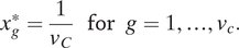 $$ {x}_g^{\ast }=\frac{1}{v_C}\hskip0.5em \mathrm{for}\hskip0.5em g=1,\dots, {v}_c. $$
With the exception of the second assumption in the next section, I do not restrict how veto groups distribute portfolios internally. Each veto group might consist of some autonomous actors, perhaps factional chiefs, who receive portfolios, along with some dependent followers, who receive no portfolios. Note that MPs who are not members of any veto group receive no portfolios.
Stage 3a: Formation of Veto Groups
If parties are unitary actors, then they will be the only veto groups in the bargaining stage. The number of veto players in this case is
 $ {v}_C=\hskip0.5em \mid C\mid $
and each coalition party’s share of the portfolios is
$ {v}_C=\hskip0.5em \mid C\mid $
and each coalition party’s share of the portfolios is
 $ \frac{1}{\mid C\mid } $
.
$ \frac{1}{\mid C\mid } $
.
At the opposite extreme, suppose that each individual MP in the coalition is an autonomous actor seeking to maximize his or her own share of offices. I characterize the process by which veto groups form, in this case of universal agency, with three axioms. The gist of these axioms is that MPs are symmetric and interchangeable, leading to equal office payoffs per MP in expectation.Footnote 4
First, since smaller veto groups get higher per-capita payoffs, I assume members form minimum-sized veto groups, those barely large enough to deprive the coalition of a majority by withholding their support. Letting
 $ {m}_C $
denote the smallest possible size of a veto group in coalition C, the coalition’s MPs will organize themselves into vC
=
$ {m}_C $
denote the smallest possible size of a veto group in coalition C, the coalition’s MPs will organize themselves into vC
=
 $ [\frac{s_C}{m_C}] $
veto groups, where
$ [\frac{s_C}{m_C}] $
veto groups, where
 $ {s}_C $
denotes the total number of seats held by coalition MPs and
$ {s}_C $
denotes the total number of seats held by coalition MPs and
 $ \left[z\right] $
denotes the greatest integer less than or equal to
$ \left[z\right] $
denotes the greatest integer less than or equal to
 $ z $
. This will leave
$ z $
. This will leave
 $ {s}_C $
–
$ {s}_C $
–
 $ {v}_C{m}_C $
MPs “out in the cold,” unable to form a veto group, where 0 ≤
$ {v}_C{m}_C $
MPs “out in the cold,” unable to form a veto group, where 0 ≤
 $ {s}_C $
–
$ {s}_C $
–
 $ {v}_C{m}_C $
<
$ {v}_C{m}_C $
<
 $ {m}_C $
.Footnote
5
$ {m}_C $
.Footnote
5
Second, if a veto group has members from more than one party, then the group divides any office spoils it receives equally among its members. This implies that the expected share of offices for an MP who belongs to a veto group will be
 $ \frac{1}{v_C}\frac{1}{m_C} $
regardless of their party.Footnote
6
Meanwhile, MPs left out in the cold will get nothing.
$ \frac{1}{v_C}\frac{1}{m_C} $
regardless of their party.Footnote
6
Meanwhile, MPs left out in the cold will get nothing.
Third, every MP is equally likely to be left out in the cold. The MPs play a giant game of musical chairs (with the veto groups being the chairs), and no MP has any advantage in finding a chair (joining a group). With this assumption, each MP’s chance of being included in a veto group is
 $ \frac{v_C{m}_C}{s_C} $
and their expected share of the portfolios, prior to the veto groups forming, is
$ \frac{v_C{m}_C}{s_C} $
and their expected share of the portfolios, prior to the veto groups forming, is
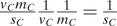 $ \frac{v_C{m}_C}{s_C}\frac{1}{v_C}\frac{1}{m_C}=\frac{1}{s_C} $
.
$ \frac{v_C{m}_C}{s_C}\frac{1}{v_C}\frac{1}{m_C}=\frac{1}{s_C} $
.
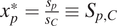
Given these assumptions, the expected portfolio share received by members of party p is
 $ {x}_p^{\ast }=\frac{s_p}{s_C}\equiv {S}_{p,C} $
. In expectation, the allocation of portfolios is strictly in accord with Gamson’s Law. If MPs really are the relevant actors, and are equally competent in chasing after office benefits, then each party’s payoff will be proportional to the number of MPs it contributes.
$ {x}_p^{\ast }=\frac{s_p}{s_C}\equiv {S}_{p,C} $
. In expectation, the allocation of portfolios is strictly in accord with Gamson’s Law. If MPs really are the relevant actors, and are equally competent in chasing after office benefits, then each party’s payoff will be proportional to the number of MPs it contributes.
As an example, consider a three-party coalition {1,2,3} with seat holdings
 $ {s}_1 $
= 30,
$ {s}_1 $
= 30,
 $ {s}_2 $
= 23, and
$ {s}_2 $
= 23, and
 $ {s}_3 $
= 12 in a 120-seat assembly. Since 61 seats are needed to control the chamber, the smallest possible veto group has
$ {s}_3 $
= 12 in a 120-seat assembly. Since 61 seats are needed to control the chamber, the smallest possible veto group has
 $ {m}_C $
= 5 members. Suppose that party 1 forms
$ {m}_C $
= 5 members. Suppose that party 1 forms
 $ \left[\frac{30}{5}\right]=6 $
veto groups with five members each, party 2 forms
$ \left[\frac{30}{5}\right]=6 $
veto groups with five members each, party 2 forms
 $ \left[\frac{23}{5}\right]=4 $
such groups, and party 3 forms
$ \left[\frac{23}{5}\right]=4 $
such groups, and party 3 forms
 $ \left[\frac{12}{5}\right]=2 $
groups. Party 2 has three remaining members who have not yet joined a veto group, while party 3 has two such members. These remaining members form a mixed-party veto group, with the participating MPs sharing office benefits equally.
$ \left[\frac{12}{5}\right]=2 $
groups. Party 2 has three remaining members who have not yet joined a veto group, while party 3 has two such members. These remaining members form a mixed-party veto group, with the participating MPs sharing office benefits equally.
If the 13 veto groups noted above form, then party 1’s portfolio share will equal its share of veto groups,
 $ \frac{6}{13} $
, which will exactly equal its seat share in the coalition:
$ \frac{6}{13} $
, which will exactly equal its seat share in the coalition:
 $ \frac{6}{13}=\frac{30}{65} $
. Party 2 will have four single-party veto groups and a three-fifth’s share in a cross-party veto group, yielding a portfolio share of
$ \frac{6}{13}=\frac{30}{65} $
. Party 2 will have four single-party veto groups and a three-fifth’s share in a cross-party veto group, yielding a portfolio share of
 $ \frac{4.6}{13} $
, which again exactly equals its seat share:
$ \frac{4.6}{13} $
, which again exactly equals its seat share:
 $ \frac{4.6}{13}=\frac{23}{65} $
. Naturally, this implies that party 3’s seat contribution and portfolio share must also exactly coincide.
$ \frac{4.6}{13}=\frac{23}{65} $
. Naturally, this implies that party 3’s seat contribution and portfolio share must also exactly coincide.
If the remaining members of party 2 and 3 do not form a cross-party veto group, then only 12 single-party veto groups will form and the portfolio payoffs will be more favorable to party 1:
 $ \frac{6}{12}>\frac{6}{13}=\frac{30}{65} $
. This example, and the theory more generally, assumes that the MPs, rather than the parties, are the actors and that they pursue every option to obtain more portfolios. Appendix A considers a version of the model in which cross-party veto groups cannot form (showing that portfolio and seat shares are still strongly related).
$ \frac{6}{12}>\frac{6}{13}=\frac{30}{65} $
. This example, and the theory more generally, assumes that the MPs, rather than the parties, are the actors and that they pursue every option to obtain more portfolios. Appendix A considers a version of the model in which cross-party veto groups cannot form (showing that portfolio and seat shares are still strongly related).
In-between unitary parties and universal agency are a continuum of cases. Following the discussion above, let β ∈ [0,1] denote how concentrated agency is in a given coalitional situation, with β = 0 corresponding to universal agency and β = 1 to unitary parties. For a given concentration of agency, each party p will have
 $ \beta +\left(1-\beta \right){s}_p $
autonomous MPs (in expectation), a number intermediate between the unitary actor assumption (one autonomous player) and the universal agency assumption (all MPs autonomous). Each autonomous MP has dependent followers, who vote as instructed. The autonomous MPs seek to form veto groups and to control them through their followers. I assume that the expected share of veto group positions controlled by an autonomous MP from party p is the same as the expected share controlled by autonomous MPs from any other party. In other words, autonomous MPs are equally good at playing the veto group formation game, regardless of which party they are in.
$ \beta +\left(1-\beta \right){s}_p $
autonomous MPs (in expectation), a number intermediate between the unitary actor assumption (one autonomous player) and the universal agency assumption (all MPs autonomous). Each autonomous MP has dependent followers, who vote as instructed. The autonomous MPs seek to form veto groups and to control them through their followers. I assume that the expected share of veto group positions controlled by an autonomous MP from party p is the same as the expected share controlled by autonomous MPs from any other party. In other words, autonomous MPs are equally good at playing the veto group formation game, regardless of which party they are in.
Given this assumption, and assuming
 $ \beta +\left(1-\beta \right){s}_p $
is an integer for all p ∈ C, party p’s share of veto group positions, and therefore its share of portfolios, will equal its share of autonomous MPs:
$ \beta +\left(1-\beta \right){s}_p $
is an integer for all p ∈ C, party p’s share of veto group positions, and therefore its share of portfolios, will equal its share of autonomous MPs:
 $$ {x}_p^{\ast }=\frac{\beta +\left(1-\beta \right){s}_p}{\sum \limits_{k\in C}\left(\beta +\left(1-\beta \right){s}_k\right)}=\frac{\beta +\left(1-\beta \right){s}_p}{\beta \mid C\mid +\left(1-\beta \right){s}_C}. $$
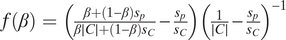
As shown in Appendix A, this can be rewritten as
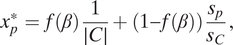 $$ {x}_p^{\ast }=f\left(\beta \right)\frac{1}{\mid C\mid }+\left(1-f\left(\beta \right)\right)\frac{s_p}{s_C}, $$
where
 $ f\left(\beta \right)\in \left[0,1\right] $
. In other words, each party p’s share of the portfolios is a convex combination of what p would get under equal sharing (
$ f\left(\beta \right)\in \left[0,1\right] $
. In other words, each party p’s share of the portfolios is a convex combination of what p would get under equal sharing (
 $ \frac{1}{\mid C\mid } $
) and what p would get under pure proportionality (
$ \frac{1}{\mid C\mid } $
) and what p would get under pure proportionality (
 $ {S}_{p,C} $
). Since equal sharing will benefit smaller parties, the equilibrium portfolio allocations predicted by the hybrid model will correspond (for appropriate values of
$ {S}_{p,C} $
). Since equal sharing will benefit smaller parties, the equilibrium portfolio allocations predicted by the hybrid model will correspond (for appropriate values of
 $ \beta $
) to the modified version of Gamson’s Law documented in the empirical literature.
$ \beta $
) to the modified version of Gamson’s Law documented in the empirical literature.
When
 $ \beta +\left(1-\beta \right){s}_p $
is not an integer for some p ∈ C, the formulas above continue to hold approximately. Consider, for example, a two-party coalition {1,2} in which party 1 has 40 seats and party 2 has 20 seats. If
$ \beta +\left(1-\beta \right){s}_p $
is not an integer for some p ∈ C, the formulas above continue to hold approximately. Consider, for example, a two-party coalition {1,2} in which party 1 has 40 seats and party 2 has 20 seats. If
 $ \beta +\left(1-\beta \right){s}_p $
is not an integer, assume that the number of autonomous MPs in party p is
$ \beta +\left(1-\beta \right){s}_p $
is not an integer, assume that the number of autonomous MPs in party p is
 $ \left[\beta +\left(1-\beta \right){s}_p\right] $
. In this case, party 1’s share of the veto positions will be
$ \left[\beta +\left(1-\beta \right){s}_p\right] $
. In this case, party 1’s share of the veto positions will be
 $ \frac{\left[\beta +\left(1-\beta \right)40\right]}{\left[\beta +\left(1-\beta \right)40\right]+\left[\beta +\left(1-\beta \right)20\right]} $
. Computing this share for values of
$ \frac{\left[\beta +\left(1-\beta \right)40\right]}{\left[\beta +\left(1-\beta \right)40\right]+\left[\beta +\left(1-\beta \right)20\right]} $
. Computing this share for values of
 $ \beta $
between 0 and 0.9, one finds that the mean absolute deviation of party 1’s portfolio share from its seat share (of 2/3) is 0.007.
$ \beta $
between 0 and 0.9, one finds that the mean absolute deviation of party 1’s portfolio share from its seat share (of 2/3) is 0.007.
Stage 2: The Formateur’s Choice of Coalition
I assume that the formateur (the leader of party f) will choose the coalition that maximizes his or her party’s share of the portfolios.Footnote 7 Let the set of minimal winning coalitions containing f be MWCf. Then the formateur’s optimal choice is
 $$ {C}_f^{\ast}\hskip0.2em \in \hskip0.2em \underset{C\hskip0.2em \in \hskip0.2em {MWC}_f}{\arg \max}\frac{\beta +\left(1-\beta \right){s}_f}{\beta \mid C\mid +\left(1-\beta \right){s}_C}\leftrightarrow {C}_f^{\ast}\hskip0.2em \in \underset{C\hskip0.2em \in \hskip0.2em {MWC}_f}{\arg \min}\beta \mid C\mid +\left(1-\beta \right){s}_C. $$
In other words, the formateur prefers “small” coalitions, either those with fewer parties or those with fewer seats, with each consideration being weighted. The more concentrated agency is within the parties, the more that the formateur focuses on minimizing the number of partners. The less concentrated agency is, the more the formateur focuses on minimizing the coalition’s seats.Footnote 8
Summary and Empirical Implications
The essence of Nash bargaining is that players have bargaining leverage if and only if they can block a deal. When parties are unitary actors, they are the only veto players, and each gets an equal share of the portfolios. If every MP is autonomous, however, then they will compete to form veto groups in order to lay claim to higher offices. My model assumes that MPs are equally successful in forming veto groups, and in claiming shares of the offices that such groups secure, regardless of which party they are from. Thus, summing MPs’ payoffs within each party leads to a prediction that each party will get a share of portfolios equal to its seat contribution to the coalition.
If all parties have similar concentrations of agency (
 $ \beta $
), then the model (see Equation 3a) predicts that portfolio shares will be a weighted average of each party’s contribution of seats and an equal share. I explore this “weighted average” model’s empirical performance below.
$ \beta $
), then the model (see Equation 3a) predicts that portfolio shares will be a weighted average of each party’s contribution of seats and an equal share. I explore this “weighted average” model’s empirical performance below.
I also explore cross-national variation in the concentration of agency within parties, due to differences in electoral rules. The question is whether electoral systems that enable more MPs to fashion autonomous electoral careers also lead to more Gamsonian portfolio allocations (per Equation 3a) and to a shift in formateurs’ preferences toward minimizing the number rather than the size of governing parties (per Equation 4).
European Portfolio Allocations: Some Evidence
Since Browne and Franklin (Reference Browne and Franklin1973), empirical studies of portfolio allocation have typically regressed each member’s portfolio share on a constant and the share of the coalition’s seats contributed by that member. The standard practice has been to estimate the model on the full sample of observations and without clustering errors. Since portfolio shares sum to one within each governing coalition, however, the errors are necessarily correlated under the standard approach. Here, I follow Fréchette, Kagel, and Morelli (Reference Fréchette, Kagel and Morelli2005) and report results for a subsample obtained by dropping one observation at random from each coalition.
Data
I use the Warwick-Druckman (Reference Warwick and Druckman2006) and Seki-Williams (Reference Seki and Williams2014) datasets, which together cover 341 cabinet formations in 14 European countries (Austria, Belgium, Denmark, Finland, France, Germany, Iceland, Ireland, Italy, Luxembourg, Netherlands, Norway, Portugal, and Sweden) over the period 1945–2012. These constitute all multiparty coalitions formed after elections in these countries in this period. Of the documented coalitions, 60 (18%) were minority coalitions, 148 (43%) were minimum winning, and 133 (39%) were oversized. After excluding one party from each cabinet at random, I was left with 694 observations on governing parties.
The Standard Specification
In Table 1, I first replicate the standard specification on my random subsample (Model 1). In this, and in all other specifications, I cluster the errors at the cabinet level.
Table 1. Portfolio Shares in Coalition Governments
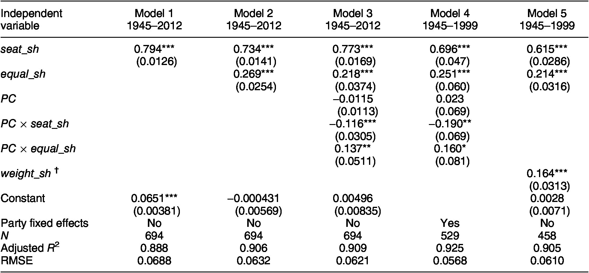
Note: One observation was removed from each cabinet in Models 1–3, and 5. In Model 4, if all parties in the cabinet satisfied the requirement of appearing in cabinet at least five times, then one observation was removed. †The variable weight_sh was merged in from Carroll and Cox’s (Reference Carroll and Cox2007) dataset. As they did not cover the full set of cases in the Warwick–Druckman data, there is some loss of observations in Model 5. *p < 0.05, **p < 0.01, ***p < 0.001.
As can be seen, Model 1 has an excellent fit, explaining 89% of the variance in the portfolio shares received by European coalition members. Also evident are two features stressed by previous researchers. First, there is a small-party bias: the constant term suggests that a vanishingly small coalition partner would still get 6.51% of the portfolios. Second, the results reveal a strong relationship between portfolio shares and seat shares. For every 1 percentage point increase in a party’s contribution of seats to a coalition, it can expect to get 0.794 percentage points more of the portfolios. This large coefficient, however, is statistically different than 1, so we can reject the hypothesis that portfolios are allocated in strict accordance with Gamson’s Law.
Model 1’s results are consistent with my theory. The strong association between portfolio and seat shares is expected if agency is widely distributed within parties. The small-party bias is expected if agency is not universal. For, in this case, coalitions will put positive weight on equal shares, thereby overcompensating small parties relative to their seat contributions. That said, the econometric model used in Model 1 is not precisely what my theory would suggest.
A New Specification: The Weighted Average Model
To implement the version of the model given in Equation 3a, one needs to add a variable (equal_sh) reflecting what each party would be “owed” under equal sharing. Model 2 displays the results of estimating such a two-principle allocative formula. As can be seen, this model appears to fit the data even better than the standard one, adding almost two percentage points to the adjusted R 2 and shaving over half a percentage point off the root mean squared error. This impression is corroborated when I use the least absolute shrinkage and selection operator to select the model, in which case (see Appendix B) both variables are included and the out-of-sample R 2 is 0.905. The estimates suggest that European coalitions placed a weight of 0.734 on their members’ seat contributions and a weight of 0.269 on the share that each member would get under equal sharing. The estimated constant term is virtually zero.Footnote 9
Model 2 is very similar to a model with “class fixed effects.” Let class z consist of all cabinets with z participating parties. Since equal_sh takes the same value for all cabinets within each class, it is similar to a model that substitutes class dummy variables in place of equal_sh. The main difference is that Model 2 has fewer variables and imposes a functional form in fitting the variation of the constant term across classes. The estimated results of a class fixed effect model (shown in Appendix B) are almost identical to those for Model 2 with respect to the slope coefficient on seat_sh and the goodness-of-fit statistics.
Candidate-Centered Electoral Rules and Gamson’s Law
My model implies that, when agency is more decentralized within parties, portfolio allocations should more closely approximate Gamson’s Law. In this section, I examine whether portfolio allocations are more Gamsonian when electoral rules make it difficult for leaders to exert unitary control over their parties.
Consider first a system in which party leaders control the nominations of their followers and in which MPs denied renomination have little prospect of electoral success. In this case, leaders “own” their parties and should be able to exert unitary control over them.Footnote 10 In contrast, in systems in which leaders exert little influence over nominations or MPs denied renomination can easily continue their electoral careers outside the party, party leaders should have much more difficulty in wielding unitary control.
To measure the extent to which leaders control nominations and MPs have poor exit options, I use Farrell and McAllister’s (Reference Farrell and McAllister2006) index of candidate centeredness. The canonical argument in the literature is that candidate-centered electoral systems motivate candidates to develop personal votes (e.g., Carey and Shugart Reference Carey and Shugart1995; Farrell and McAllister Reference Farrell and McAllister2006). Here, I simply point out two corollaries of this observation. First, politicians’ post-exit prospects improve as their personal followings increase. Thus, MPs should have better exit options in more candidate-centered electoral systems. Second, leaders should find it harder to exert nomination control over politicians with personal followings. Such politicians can use their personal followings to promote their own renomination, and denying them renomination may simply prompt them to leave the party. Thus, in candidate-centered electoral systems, leaders should be less able to manipulate nominations in order to pack the party with dependents.
In contrast, party-centered electoral systems tend to both worsen MPs’ exit options and improve leaders’ control over nominations. In closed-list PR systems, for example, exiting candidates can rarely expect to receive a winnable spot on another party’s list, and party leaders typically exert substantial influence over who gets winnable list positions. Thus, leaders are better positioned to concentrate agency within their own hands.Footnote 11
All told, I expect that candidate-centered systems will decentralize agency, thereby promoting portfolio allocations that better approximate Gamson’s Law. To explore this hypothesis, I dichotomize the Farrell–McAllister index, with all countries scoring above their midpoint value of 5 being “candidate-centered” and the rest being “party-centered.” Of the 14 countries in my sample, six have candidate-centered electoral systems by this standard—Denmark, Finland, France, Ireland, Italy, and Luxembourg. Another eight countries have party-centered systems—Austria, Belgium, Germany, Iceland, Netherlands, Norway, Portugal, and Sweden. The Carey–Shugart (Reference Carey and Shugart1995) index yields the same dichotomous classification (although it differs at a finer level of classification, as explained by Farrell and McAllister Reference Farrell and McAllister2006).
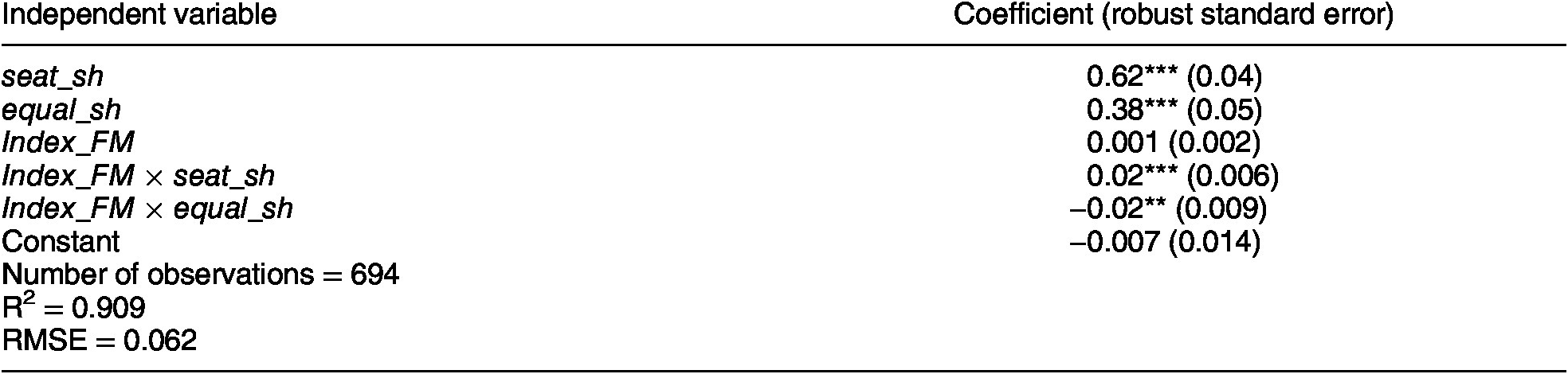
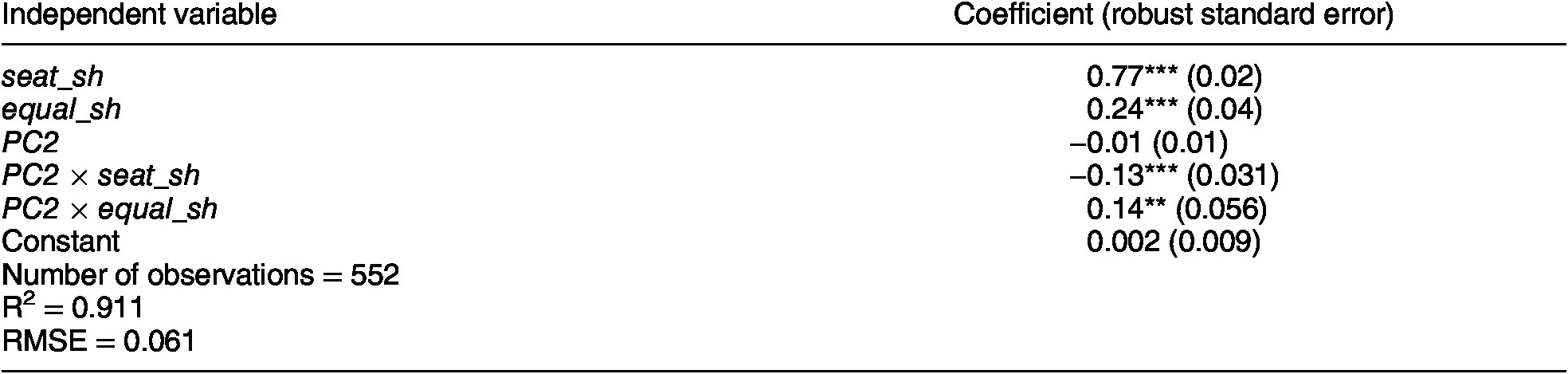
In Model 3, I let the coefficients in Model 2 shift between the party- and candidate-centered systems. In particular, letting PC = 1 if a party competes in a party-centered electoral system (and = 0 otherwise), I run the following regression:
 $$ Portfolio\_ sh=\unicode{x03B1} +{\unicode{x03B2}}_1 seat\_ sh+{\unicode{x03B2}}_2 equal\_ sh+{\unicode{x03B3}}_1 PC\hskip1.3em +{\unicode{x03B3}}_2\mathrm{PC}\times seat\_ sh+{\unicode{x03B3}}_3 PC\times equal\_ sh+\unicode{x025B} . $$
The results show that portfolio allocations in candidate-centered systems more closely approximate Gamson’s Law. The coefficient on seat share is 0.77, versus 0.66 in party-centered systems, and the coefficient on equal shares is 0.22, versus 0.36 in the party-centered systems.
Similar results hold if PC is replaced by the Farrell–McAllister index (see Appendix C). In other words, dichotomizing their index does not drive my results. That said, I prefer dichotomizing because, as Farrell and McAllister note, there is no natural cardinal meaning to their index scores.
My results are also robust to recoding the Netherlands as affording exit options similar to those in the candidate-centered cases. The rationale for such a recoding is that the Netherlands has such a high district magnitude (150) that tiny splinter parties can form and expect to have electoral success. The consequence of such a recoding is to slightly strengthen the results (as shown in Appendix D).
No one has previously explored whether electoral rules affect the extent to which governments’ portfolio allocations follow Gamson’s Law because no one has argued that the intraparty concentration of agency affects leaders’ bargaining positions in interparty negotiations. The results presented here suggest that it will be worth further exploring the connections between the intraparty decentralization of agency and the outcome of interparty negotiations.
Variations in Intraparty Democracy?
The Farrell–McAllister index varies only at the country level, and one might wonder whether parties within each country differed significantly in their concentration of agency (even after controlling for the common electoral incentives facing them all). In Model 4, I restrict the analysis to parties that participated in government at least five times during the period 1945–1999 and use party fixed effects to control for each party’s concentration of agency.Footnote 12 Party fixed effects help control for two theoretically relevant factors—the variation across countries in electoral rules and the variation across parties (within a given country) in how much leverage their rules give to factions.
As can be seen, even controlling for party fixed effects, the estimated effects are very similar to those in Model 3. In other words, estimating the effects using only within-party variation (Model 4) yields the same basic picture as estimating the effects using cross-sectional comparisons (Model 3).
I do not report the estimated party fixed effects, but they are of some interest. If a given country’s factions have similar leverage regardless of which party they belong to—either because the electoral system is the main determinant of factional leverage or all parties have similar internal rules—then party fixed effects will cluster within countries. A simple test of clustering is to compare the range of party fixed effects in each country with the range across the entire dataset. The average within-country range is about 43% of the overall range, suggesting that cross-country differences dominate.
Voting Weights
I will discuss Model 5 later. For the moment, suffice it to say that when one adds to Model 2 a control for each party’s share of voting weight in the coalition, previous results remain qualitatively similar and the new variable is also significant.
Party-Centered Electoral Systems and the Formateur’s Choice
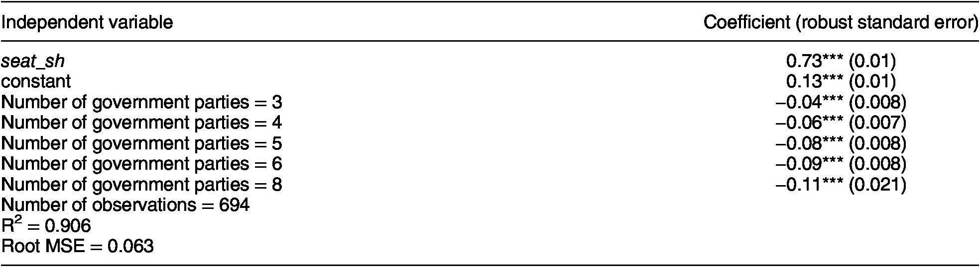
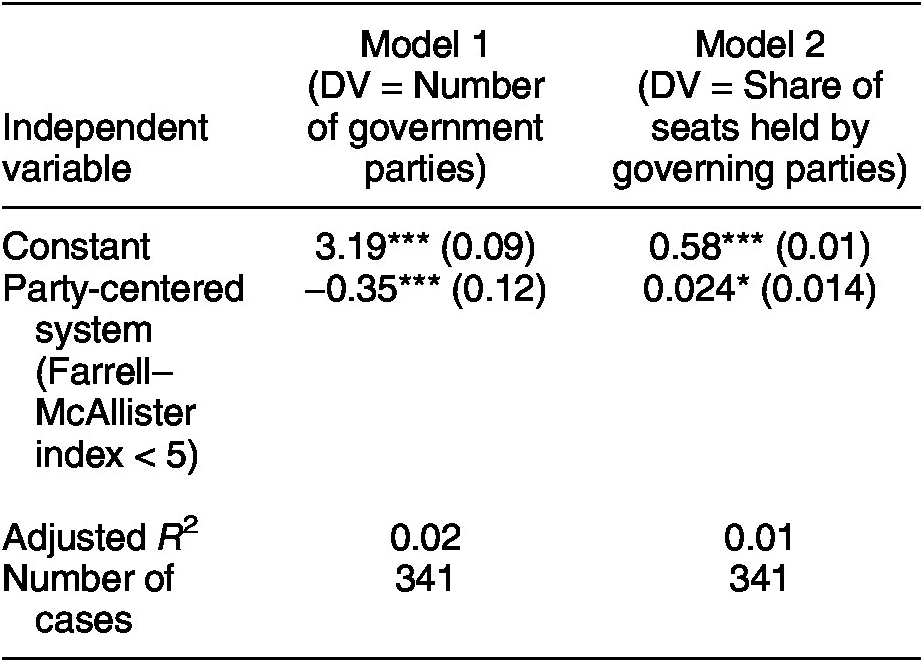
My model suggests (see Equation 4) that formateurs in party-centered electoral systems will focus on minimizing the number of parties they invite to form a government, while formateurs in candidate-centered systems will put more weight on minimizing the share of seats collectively held by governing parties. I investigate these predictions, using bivariate regressions, in Table 2.
Table 2. Party-Centered Electoral Systems and the Size of Governments

Note: *p < 0.10, **p < 0.05, ***p < 0.01
As can be seen, the number of governing parties tends to be systematically smaller in party- as opposed to candidate-centered electoral systems (see Model 1). Meanwhile, the opposite pattern holds with respect to the share of seats held by governing parties (see Model 2). There are many possible confounders in these analyses, but the theoretical predictions are nonobvious and the empirical results turn out as expected.
Existing Explanations of Gamson’s Law
To the best of my knowledge, the theory of government formation offered here is the first that (for some parameter values) directly implies the long-standing empirical finding of proportional allocations modified by small-party bias.Footnote 13 In this section, I review previous explanations, commenting on their relationship to my approach.
Expectations
Gamson’s original argument (Reference Gamson1961, 376) was that bargainers would expect others to demand a share of output proportional to the resources they contribute. Applied to government formation, this means that political parties expect each other to demand a share of cabinet portfolios proportional to the seats they contribute to the coalition. Gamson did not, however, formally prove that bargainers with such expectations would agree on a proportional allocation. Moreover, when a formal analysis of demand bargaining was conducted (Morelli Reference Morelli1999), the analysis showed that the unique equilibrium involved an allocation proportional to voting weights (a nonlinear function of seats), not an allocation proportional to seats. In other words, the expectations that Gamson posited were not sustainable in Nash equilibrium (in Morelli’s model).
Social Norms and Bargaining Conventions
Some scholars argue that proportional allocation is a “bargaining convention” (Bäck, Meier, and Persson Reference Bäck, Meier and Persson2009) or a “focal point” (Falcó-Gimeno and Indridason Reference Falcó-Gimeno and Indridason2013). The idea is that bargainers use proportionality as a way to coordinate on one equilibrium when many equilibria exist. In contrast, in my model jockeying for position among autonomous MPs pins down a unique equilibrium. Since multiple equilibria do not exist, no convention is needed to select among them.Footnote 14
Formateurs’ Incentives
Several scholars focus on explaining why formateurs will not exploit their proposal powers to extract bonuses, as the Baron–Ferejohn (Reference Baron and Ferejohn1989) model suggests they should. One idea is that the parties in each coalition compete to become the formateur and, in the process, dissipate the rents (Bassi Reference Bergman2013). Another idea is that formateurs seek to build coalitions that can survive votes of no confidence, which leads them to overcompensate smaller partners (Golder and Thomas Reference Golder and Thomas2014; Indridason Reference Indridason2015).
Following the advice of Laver, de Marchi, and Mutlu (Reference Laver, de Marchi and Mutlu2011), my model dispenses with the assumption that formateurs have structural proposal power. Thus, there is no need to explain why they do not exploit that power.
Audience Costs
Martin and Vanberg (Reference Martin and Vanberg2020, 1140) consider a model in which some voters will punish their own party, if it fails to obtain as many portfolios as those voters think it should in a particular coalition. When such voters expect parties to get portfolios in proportion to their seats—one of several performance yardsticks that Martin and Vanberg consider—party leaders have strong incentives to obtain a Gamsonian allocation and avoid punishment at the polls.
As in Gamson’s original explanation, Martin and Vanberg assume that some agents expect parties to demand proportional shares of portfolios. Unlike Gamson, however, Martin and Vanberg’s posited expectations can be realized in equilibrium—because voters’ responses to their parties’ failure to obtain proportional shares pose exogenous constraints on the negotiators seeking to form coalition governments. That said, how close the approximation to Gamson’s Law will be under the Martin–Vanberg model depends on how sharply voter support drops off for parties failing to get proportional shares.Footnote 15
Moral Hazard
Carroll and Cox (Reference Carroll and Cox2007) share the present paper’s assumption that mobilizing votes in support of a coalition is costly. However, they consider mobilizing votes in general elections (rather than within parliament) and assume that mobilizational effort is unobservable. This leads them to focus most of their attention on the moral hazard problems that beset coalitions. Their main argument is that, if a coalition commits to a more Gamsonian distribution of portfolios, then all its component parties will have stronger incentives to win seats, thereby improving the coalition’s chances of winning a majority.
Vote mobilization efforts are imperfectly observable within parliament, too (Laver Reference Laver1999). So, Gamsonian allocations may be useful in mitigating moral hazard within teams of parliamentary mobilizers, too. Here, however, I have stressed just the costliness of mobilization, when not all MPs are dependent on their leaders, rather than the unobservability of effort.
Extensions
The model sketched above is flexible enough to accommodate different assumptions at various points. In this section, I consider two extensions—allowing disagreement payoffs (
 $ {d}_g $
) to vary across veto groups and allowing the distribution of agency (β) to vary across parties.
$ {d}_g $
) to vary across veto groups and allowing the distribution of agency (β) to vary across parties.
Bargaining When Disagreement Payoffs Vary
The baseline model assumes that all bargainers have disagreement payoffs of zero. In this section, I take veto group
 $ g $
’s disagreement payoff as an exogenously given nonnegative parameter
$ g $
’s disagreement payoff as an exogenously given nonnegative parameter
 $ {d}_g $
reflecting the value of the group members’ opportunities in the event that the current coalition fails to reach agreement and another formateur is appointed.Footnote
16
One can think of these disagreement payoffs as reflecting each group’s pivotality—the number of different minimum winning coalitions to which the group belongs. The NBS payoffs in this case are
$ {d}_g $
reflecting the value of the group members’ opportunities in the event that the current coalition fails to reach agreement and another formateur is appointed.Footnote
16
One can think of these disagreement payoffs as reflecting each group’s pivotality—the number of different minimum winning coalitions to which the group belongs. The NBS payoffs in this case are
 $$ {x}_g^{\ast }={DD}_g+\left(1-D\right)\frac{1}{v_C}. $$
Here,
 $ D=\sum \limits_g{d}_g $
is the amount needed to compensate all veto groups for their opportunity costs (their payoffs given disagreement), and
$ D=\sum \limits_g{d}_g $
is the amount needed to compensate all veto groups for their opportunity costs (their payoffs given disagreement), and
 $ {D}_g=\frac{d_g}{D} $
is
$ {D}_g=\frac{d_g}{D} $
is
 $ g $
’s share of the opportunity-cost compensations (or share of pivotality).
$ g $
’s share of the opportunity-cost compensations (or share of pivotality).
Assuming that
 $ D\hskip0.5em \le \hskip0.5em 1 $
(the opportunity-cost payments are no more than the value of the portfolios), each veto group’s payoff is a weighted average of what they would get under equal sharing and their share of the opportunity-cost payments. Aggregating up to the party level, each party p’s share of portfolios will be a weighted average of three components: p’s share of seats contributed, p’s share of external opportunity values, and p’s egalitarian share. Model 5 in Table 1 displays the results of estimating this three-component allocative formula, where p’s share of external opportunity values is measured operationally as its share of voting weight. As can be seen, this model fits the data about as well as Model 2, and all three factors are significant predictors of portfolio shares. The results suggest that coalitions place the largest weight on seat contributions, the next largest weight on equal sharing, and the smallest weight on pivotality.Footnote
17
$ D\hskip0.5em \le \hskip0.5em 1 $
(the opportunity-cost payments are no more than the value of the portfolios), each veto group’s payoff is a weighted average of what they would get under equal sharing and their share of the opportunity-cost payments. Aggregating up to the party level, each party p’s share of portfolios will be a weighted average of three components: p’s share of seats contributed, p’s share of external opportunity values, and p’s egalitarian share. Model 5 in Table 1 displays the results of estimating this three-component allocative formula, where p’s share of external opportunity values is measured operationally as its share of voting weight. As can be seen, this model fits the data about as well as Model 2, and all three factors are significant predictors of portfolio shares. The results suggest that coalitions place the largest weight on seat contributions, the next largest weight on equal sharing, and the smallest weight on pivotality.Footnote
17
Bargaining When Intraparty Agency Varies
My model assumes that all parties have equal distributions of agency (β). To the extent that factional leverage depends mostly on exit options, this assumption would be valid—since the same electoral rules apply to all parties.
If parties’ internal rules also have an important influence on internal agency, then my model would imply that formateurs will try to avoid parties with more internal veto players, seats held constant. Bäck (Reference Bäck2008) provides some evidence that formateurs do behave in this way. Investigating coalition formation at the local level in Sweden, she finds that “parties are less likely to be in government the higher their level of factionalization and the higher their level of intra-party democracy” (72). To the extent that factionalization and intraparty democracy indicate wider agency within the party, her results are consistent with my model.
Policy Payoffs
One can reinterpret the bargaining subgame (Stage 3b) as referring not to an allocation of offices but rather to an allocation of “decision-making influence.” Under this interpretation, each veto group has an equal opportunity to propose an allocation of influence,
 $ y=\left({y}_1,\dots, {y}_{v_C}\right\} $
, where
$ y=\left({y}_1,\dots, {y}_{v_C}\right\} $
, where
 $ {y}_g\hskip0.3em \in \hskip0.3em \left[0,1\right] $
and
$ {y}_g\hskip0.3em \in \hskip0.3em \left[0,1\right] $
and
 $ \sum \limits_g{y}_g=1 $
. If everyone accepts a proposal, then the coalition policy that results is
$ \sum \limits_g{y}_g=1 $
. If everyone accepts a proposal, then the coalition policy that results is
 $ z(y)=\sum \limits_g{y}_g{z}_g $
, where
$ z(y)=\sum \limits_g{y}_g{z}_g $
, where
 $ {z}_g $
is veto group
$ {z}_g $
is veto group
 $ g $
’s ideal point. In other words, greater influence allows a group to pull the coalition’s platform closer to its ideal policy. As in Laver and Shepsle (Reference Laver and Shepsle1996), how offices are allocated automatically affects the policies that coalitions will follow—although here policy effects are given a reduced-form representation. If anyone rejects a proposal, then another veto group is equi-probably recognized to make a proposal. As long as bargainers fail to agree on a division of influence, they all receive zero payoffs (the status quo remains in force).
$ g $
’s ideal point. In other words, greater influence allows a group to pull the coalition’s platform closer to its ideal policy. As in Laver and Shepsle (Reference Laver and Shepsle1996), how offices are allocated automatically affects the policies that coalitions will follow—although here policy effects are given a reduced-form representation. If anyone rejects a proposal, then another veto group is equi-probably recognized to make a proposal. As long as bargainers fail to agree on a division of influence, they all receive zero payoffs (the status quo remains in force).
Why do leaders value influence? One interpretation is that policy is one dimensional and all parties have linear spatial utilities so that influence turns linearly into “policy gains.” To illustrate, let
 $ {\Delta}_g\left(z(y)\right) $
denote group
$ {\Delta}_g\left(z(y)\right) $
denote group
 $ g $
’s policy gain if the policy
$ g $
’s policy gain if the policy
 $ z(y) $
is agreed upon. I shall rewrite
$ z(y) $
is agreed upon. I shall rewrite
 $ z(y) $
=
$ z(y) $
=
 $ {y}_g{z}_g+\left(1-{y}_g\right){z}_{-g} $
, where
$ {y}_g{z}_g+\left(1-{y}_g\right){z}_{-g} $
, where
 $ {z}_{-g} $
=
$ {z}_{-g} $
=
 $ \sum \limits_{k\ne g}\frac{y_k{z}_k}{1-{y}_g} $
is the policy outcome that would result if
$ \sum \limits_{k\ne g}\frac{y_k{z}_k}{1-{y}_g} $
is the policy outcome that would result if
 $ g $
’s weight were reduced to zero and all others’ weights scaled up proportionately. Adopting the normalizations
$ g $
’s weight were reduced to zero and all others’ weights scaled up proportionately. Adopting the normalizations
 $ {z}_{-g} $
= 0 and
$ {z}_{-g} $
= 0 and
 $ {z}_g $
= 1, one can write
$ {z}_g $
= 1, one can write
 $ z(y) $
=
$ z(y) $
=
 $ {y}_g $
. Now let
$ {y}_g $
. Now let
 $ g $
’s utility function satisfy
$ g $
’s utility function satisfy
 $ {V}_g(z) $
=
$ {V}_g(z) $
=
 $ 1-\left(1-z\right)=z $
for all
$ 1-\left(1-z\right)=z $
for all
 $ z\in \left[0,1\right] $
, and
$ z\in \left[0,1\right] $
, and
 $ {V}_g(z) $
= 0 for
$ {V}_g(z) $
= 0 for
 $ z\notin \left[0,1\right] $
. The policy gain is then
$ z\notin \left[0,1\right] $
. The policy gain is then
 $ {\Delta}_g\left(z(y)\right) $
=
$ {\Delta}_g\left(z(y)\right) $
=
 $ {V}_g\left(z(y)\right) $
–
$ {V}_g\left(z(y)\right) $
–
 $ {V}_g(q) $
, where q is the status quo policy. This reduces to
$ {V}_g(q) $
, where q is the status quo policy. This reduces to
 $ {\Delta}_g\left(z(y)\right) $
=
$ {\Delta}_g\left(z(y)\right) $
=
 $ {y}_g $
if
$ {y}_g $
if
 $ q\notin \left[0,1\right] $
.
$ q\notin \left[0,1\right] $
.
Given linear policy payoffs, bargaining over shares of influence is similar to bargaining over office shares. Every veto group
 $ g $
will have an equal influence in equilibrium. Aggregating within parties, each party’s influence over the coalition’s platform will be a weighted average of the share of seats it contributes to the coalition and an equal share. When allocations of influence put most of the weight on seat proportionality, the equilibrium policy outcome
$ g $
will have an equal influence in equilibrium. Aggregating within parties, each party’s influence over the coalition’s platform will be a weighted average of the share of seats it contributes to the coalition and an equal share. When allocations of influence put most of the weight on seat proportionality, the equilibrium policy outcome
 $ z\left({y}^{\ast}\right) $
will be a weighted average of the parties’ ideal points, with the weights determined mostly by each party’s contribution of seats to the coalition.
$ z\left({y}^{\ast}\right) $
will be a weighted average of the parties’ ideal points, with the weights determined mostly by each party’s contribution of seats to the coalition.
This theoretical result resonates with several findings in the empirical literature. For example, in his investigation of policies within multiparty European coalitions, Warwick (Reference Warwick2001, 1215; see also Martin and Vanberg Reference Martin and Vanberg2014) found that “coalition policy corresponds with the weighted mean position of the parties in government, with parties’ seat share constituting the weights.” Similarly, in his investigation of policies within multifactional parties, Ceron (Reference Ceron2012, 691) found that “the mean of factions’ positions weighted by the size of each faction” was a good predictor.
Conclusion
In this paper, I have introduced a new model of government formation based on two main assumptions. First, no actor has a structural advantage in the negotiations leading to government formation. Instead, the bargaining protocol used is entirely neutral between the actors involved. Second, forming a coalition is not simply a matter of party leaders meeting and agreeing a deal. A variety of intraparty and even cross-party lobbying groups will seek to influence the outcome. I take this to a logical extreme in which every autonomous MP in the coalition seeks to form a veto group in order to increase their leverage in the bargaining over office benefits.
Compte and Jehiel (Reference Compte and Jehiel2010) have shown that the neutral bargaining protocol I posit noncooperatively implements the NBS. Under the NBS, parties’ portfolio shares are a weighted average of their seat contributions and an equal share. Theoretically, mine is the first bargaining model that directly implies the pattern found in the empirical literature: portfolio allocations are mostly proportional to each party’s seat contributions, but small parties tend to do better than their contributions alone would justify. It thus addresses the “portfolio allocation paradox” noted by Warwick and Druckman (Reference Warwick and Druckman2006).
In addition to providing a theoretical explanation for a modified Gamson’s Law, my model also implies that party leaders’ ability to control their members’ electoral careers should affect how coalitions allocate portfolios. I have provided evidence consistent with this hypothesis, showing that portfolio allocations are more Gamsonian in candidate-centered electoral systems.
The model presented here is abstract enough to apply to many other “voting teams” whose members contribute costly mobilizational effort to win elections then use neutral bargaining protocols to divide the spoils of victory. It may thus help explain why Gamsonian allocations have been documented across the members of several different types of voting team sharing several different types of resource. Parties in preelectoral coalitions share both winnable nominations (D’Alimonte Reference D’Alimonte, Gallagher and Mitchell2005) and portfolios (Carroll and Cox Reference Carroll and Cox2007) in proportion to seat contributions. Parties within governing coalitions share both portfolios (as considered here) and managerial board positions in state-owned enterprises (Ennser-Jedenastik Reference Ennser-Jedenastik2014) in proportion to seat contributions. Both factions and regional branches within parties share portfolios in proportion to seat contributions (see Ceron Reference Ceron2014; Leiserson Reference Leiserson1968; and Mershon Reference Mershon2001a; Reference Mershon2001b on factions; see Ennser-Jedenastik Reference Ennser-Jedenastik2013 on regional branches). Even individual candidates on closed lists appear to be promised rewards in proportion to their electoral contributions (Cox et al. Reference Cox, Fiva, Smith and Sørensen2020).
DATA AVAILABILITY STATEMENT
Replication files are available at the American Political Science Review Dataverse: https://doi.org/10.7910/DVN/RQE9SO.
ACKNOWLEGDMENTS
I thank Avi Acharya, Jon Fiva, Mik Laver, Scott de Marchi, and Dan Smith for their helpful comments and Jamie Druckman and Paul Warwick for sharing their data.
CONFLICT OF INTEREST
The author declares no ethical issues or conflicts of interest in this research.
ETHICAL STANDARDS
The author affirms that this research did not involve human participants.
Appendix A: Office allocations when veto groups can form only within parties
The baseline model assumes that veto groups can contain members of different parties. While cross-party cooperation between factions is not unheard of, there may be some interest in exploring office allocations when veto groups can form only within parties. In this case, if we sum the veto groups’ payoffs within party p, we get an overall allocation to party p of:
 $$ {x}_{p,C}^{\ast }=\frac{\left[\frac{s_p}{m_C}\right]}{\sum \limits_{k\in C}\left[\frac{s_k}{m_C}\right]}\mathrm{for}\hskip0.5em p\hskip0.15em \in \hskip0.15em C $$
The portfolio payoffs in Equation A.1 are those that would result if ministers were elected via a whole-quota-based method of proportional representation, with
 $ {m}_C $
being the quota. As long as party seat totals are generally “large” relative to
$ {m}_C $
being the quota. As long as party seat totals are generally “large” relative to
 $ {m}_C $
, each party’s portfolio allocation will be near to its seat contribution,
$ {m}_C $
, each party’s portfolio allocation will be near to its seat contribution,
 $ {S}_{p,C} $
. Thus, Gamson’s Law will hold approximately.
$ {S}_{p,C} $
. Thus, Gamson’s Law will hold approximately.
Derivation of Equation 3b from Equation 3a.
Suppose that
 $ \frac{\beta +\left(1-\beta \right){s}_p}{\beta \mid C\mid +\left(1-\beta \right){s}_C} $
 $ =f\left(\beta \right)\frac{1}{\mid C\mid }+\left(1-f\left(\beta \right)\right)\frac{s_p}{s_C} $
. Assuming that
$ =f\left(\beta \right)\frac{1}{\mid C\mid }+\left(1-f\left(\beta \right)\right)\frac{s_p}{s_C} $
. Assuming that
 $ \frac{1}{\mid C\mid }-\frac{s_p}{s_C}\ne 0 $
and solving for
$ \frac{1}{\mid C\mid }-\frac{s_p}{s_C}\ne 0 $
and solving for
 $ f\left(\beta \right) $
, we get
$ f\left(\beta \right) $
, we get
 $ f\left(\beta \right)=\left(\frac{\beta +\left(1-\beta \right){s}_p}{\beta \mid C\mid +\left(1-\beta \right){s}_C}-\frac{s_p}{s_C}\right){\left(\frac{1}{\mid C\mid }-\frac{s_p}{s_C}\right)}^{-1} $
. If
$ f\left(\beta \right)=\left(\frac{\beta +\left(1-\beta \right){s}_p}{\beta \mid C\mid +\left(1-\beta \right){s}_C}-\frac{s_p}{s_C}\right){\left(\frac{1}{\mid C\mid }-\frac{s_p}{s_C}\right)}^{-1} $
. If
 $ \frac{1}{\mid C\mid }-\frac{s_p}{s_C}>0 $
, then
$ \frac{1}{\mid C\mid }-\frac{s_p}{s_C}>0 $
, then
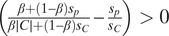 $ \left(\frac{\beta +\left(1-\beta \right){s}_p}{\beta \mid C\mid +\left(1-\beta \right){s}_C}-\frac{s_p}{s_C}\right)>0 $
for all
$ \left(\frac{\beta +\left(1-\beta \right){s}_p}{\beta \mid C\mid +\left(1-\beta \right){s}_C}-\frac{s_p}{s_C}\right)>0 $
for all
 $ \beta $
> 0, and
$ \beta $
> 0, and
 $ f\left(\beta \right)\in \left[0,1\right] $
for
$ f\left(\beta \right)\in \left[0,1\right] $
for
 $ \beta \in \left[0,1\right] $
. If
$ \beta \in \left[0,1\right] $
. If
 $ \frac{1}{\mid C\mid }-\frac{s_p}{s_C}<0 $
, then
$ \frac{1}{\mid C\mid }-\frac{s_p}{s_C}<0 $
, then
 $ \left(\frac{\beta +\left(1-\beta \right){s}_p}{\beta \mid C\mid +\left(1-\beta \right){s}_C}-\frac{s_p}{s_C}\right)<0 $
for all
$ \left(\frac{\beta +\left(1-\beta \right){s}_p}{\beta \mid C\mid +\left(1-\beta \right){s}_C}-\frac{s_p}{s_C}\right)<0 $
for all
 $ \beta $
> 0, and again
$ \beta $
> 0, and again
 $ f\left(\beta \right)\hskip0.15em \in \hskip0.15em \left[0,1\right] $
for
$ f\left(\beta \right)\hskip0.15em \in \hskip0.15em \left[0,1\right] $
for
 $ \beta \hskip0.15em \in \hskip0.15em \left[0,1\right] $
. Finally, if
$ \beta \hskip0.15em \in \hskip0.15em \left[0,1\right] $
. Finally, if
 $ \frac{1}{\mid C\mid }-\frac{s_p}{s_C}=0 $
, then
$ \frac{1}{\mid C\mid }-\frac{s_p}{s_C}=0 $
, then
 $ \frac{\beta +\left(1-\beta \right){s}_p}{\beta \mid C\mid +\left(1-\beta \right){s}_C} $
=
$ \frac{\beta +\left(1-\beta \right){s}_p}{\beta \mid C\mid +\left(1-\beta \right){s}_C} $
=
 $ \frac{1}{\mid C\mid } $
, and any value of
$ \frac{1}{\mid C\mid } $
, and any value of
 $ f\left(\beta \right)\hskip0.15em \in \hskip0.15em \left[0,1\right] $
will work.
$ f\left(\beta \right)\hskip0.15em \in \hskip0.15em \left[0,1\right] $
will work.
Appendix B: Lasso linear analysis
Using the “lasso linear” command in Stata, one can explore whether both equal_sh and seat_sh belong in the model. The results show that both variables are selected for inclusion, with an out-of-sample R2 of .905 and a cross-validated prediction error of .00402.
Linear regression with class fixed effects
Standard errors adjusted for 341 clusters (by cabinet identification number)
Appendix C: Using the Farrell-McAllister Index
Note: Standard errors adjusted for 341 clusters (by cabinet identification number). The sign flips, relative to that in Table 1, because the index is coded so that larger values indicate more candidate-centered systems.
Appendix D: Model with Netherlands re-coded
Note: Standard errors adjusted for 274 clusters (by cabinet identification number). In this analysis, PC2 = PC except that the Netherlands is counted as a candidate-centered electoral system.


Comments
No Comments have been published for this article.