


Introduction
Emotions influence political behavior. Anxiety has been shown to stimulate preferences for protective policies (Albertson and Gadarian Reference Albertson and Gadarian2015), increase support for conservative male candidates (Holman, Merolla, and Zechmeister Reference Holman, Merolla and Zechmeister2016; Holman et al. Reference Holman, Merolla, Zechmeister and Wang2019) and incumbents (Morgenstern and Zechmeister Reference Morgenstern and Zechmeister2001), and generally prompt voters to consider their choices more carefully (MacKuen et al. Reference MacKuen, Marcus, Neuman, Keele, Neuman, Marcus, Crigler and MacKuen2007; Marcus, Neuman, and MacKuen Reference Marcus, Neuman and MacKuen2000). In this paper, we build upon and extend existing theory by proposing that voters engage in a general “flight to safety” when faced with anxiety-inducing exogenous shocks. Substantively, our framework predicts that voters move toward the status quo under times of threat. This flight to safety is broader than a simple preference for incumbents, particular candidate attributes, or candidates’ policy platforms.
Our argument carries provocative implications for democratic accountability and governance. If and where a flight to safety operates, candidates who offer to preserve the status quo will find an easier path to (re-)election, regardless of whether their policy platforms are favored by the electorate on substantive grounds. In addition, strategic actors may attempt to manipulate anxiety in order to pursue political outcomes that would otherwise be unattainable. And where the prospect of change is itself a potential source of anxiety—as psychology suggests it often may be (Jost and Hunyady Reference Jost and Hunyady2003; Paterson and Cary Reference Paterson and Cary2002)—a flight to safety may be a feedback mechanism that adds friction to efforts to disrupt the status quo, making radical change more difficult.
We test our argument using a variety of empirical contexts and methods. Our primary analysis uses a staggered primary election, the timing of which was decided independently of the COVID-19 pandemic: the 2020 Democratic primary election in the United States.Footnote 1 We show that our hypothesized political flight to safety is meaningfully predictive of the antiestablishment candidate Bernie Sanders’s electoral fortunes relative to those of his primary rival, Joe Biden. To isolate our theorized causal mechanism, we field a survey experiment in which we randomize the policy platform and status quo qualities of two hypothetical candidates. We assign half of our respondents to a treatment condition that emphasizes the anxiety-inducing qualities of the COVID-19 pandemic and the other half to a reassuring frame that emphasizes progress made on finding a vaccine. Again, we find evidence consistent with a political flight to safety that is independent of the policy platforms of the two hypothetical candidates. Finally, we test the generalizability of our findings by documenting similar patterns in the 2020 primary elections for the House of Representatives with more antiestablishment candidates garnering disproportionately less support when their elections were held after the spread of COVID-19. Similarly, we examine the fortunes of more mainstream and more antiestablishment French political parties in their 2020 municipal elections, finding that more antiestablishment parties lost support in the June 2020 round of elections relative to their fortunes in early March.
Across these settings we find consistent evidence of an electoral penalty for nonmainstream candidates and parties. We consider and reject plausible alternative mechanisms, providing suggestive evidence that our interpretation of the findings—a “flight to safety”—is most consistent with the empirical evidence. These results are substantively quite large, with the magnitude of the vote shift ranging from 2 to 15 percentage points across our empirical contexts. We conclude that the political flight to safety is an important, but not yet fully accounted for, phenomenon in voting behavior.
Theory and Empirical Contexts
Market analysts refer to a “flight to safety” to describe the behavior of investors in the face of uncertainty (Adrian, Crump, and Vogt Reference Adrian, Crump and Vogt2019; Inghelbrecht et al. Reference Inghelbrecht, Bekaert, Baele and Wei2013). As market outcomes become more uncertain, investors shift toward more liquid and government-insured assets, which are perceived as safer (Cohn et al. Reference Cohn, Engelmann, Fehr and Maréchal2015). We hypothesize that a similar flight to safety operates in the market for political candidates.
We center our intuition on a spatial model of voting with valence (Ansolabehere and Snyder Reference Ansolabehere and Snyder2000; Downs Reference Downs1957; Krehbiel Reference Krehbiel1998), given in Equation 1. In this framework, voter i’s utility for supporting candidate j on issue k is some combination of policy preferences and the candidate’s valence attributes. The policy component is the classic spatial model of voting where utility is declining in the distance between the voter’s preferred policy (
 $ {\theta}_k^{\ast } $
) and the platform of candidate j (θj,k
), where the shape of the decline is parameterized with α.
Footnote
2
The valence component Vj
represents nonpolicy candidate qualities like charisma, leadership, or—in our framework—safety.
$ {\theta}_k^{\ast } $
) and the platform of candidate j (θj,k
), where the shape of the decline is parameterized with α.
Footnote
2
The valence component Vj
represents nonpolicy candidate qualities like charisma, leadership, or—in our framework—safety.
 $$ {u}_{i,j,k}=\underset{Policy}{\underbrace{-\left(1-w\right){\left({\theta}_{j,k}-{\theta}_k^{\ast}\right)}^{\alpha }}}+\underset{Valence}{\underbrace{wV_j}}. $$
Existing political science work on anxiety focuses attention on different parts of this model. One branch of the literature suggests that anxiety affects political behavior by shifting the voter’s policy preferences
 $ {\theta}_k^{\ast } $
toward “protective policies,” benefiting conservative candidates whose platforms (θj,k
) are more likely to emphasize these dimensions (e.g., Albertson and Gadarian Reference Albertson and Gadarian2015; Clifford and Jerit Reference Clifford and Jerit2018; Stenner Reference Stenner2005). Empirical work in this vein shows that crises such as terrorist attacks (Getmansky and Zeitzoff Reference Getmansky and Zeitzoff2014) and public health threats (Campante, Depetris-Chauvin, and Durante Reference Campante, Depetris-Chauvin and Durante2020) disproportionately benefit conservatives.
$ {\theta}_k^{\ast } $
toward “protective policies,” benefiting conservative candidates whose platforms (θj,k
) are more likely to emphasize these dimensions (e.g., Albertson and Gadarian Reference Albertson and Gadarian2015; Clifford and Jerit Reference Clifford and Jerit2018; Stenner Reference Stenner2005). Empirical work in this vein shows that crises such as terrorist attacks (Getmansky and Zeitzoff Reference Getmansky and Zeitzoff2014) and public health threats (Campante, Depetris-Chauvin, and Durante Reference Campante, Depetris-Chauvin and Durante2020) disproportionately benefit conservatives.
A related body of work focuses on risk aversion and how heterogeneity in risk appetite influences voting behavior (Eckel, El-Gamal, and Wilson Reference Eckel, El-Gamal and Wilson2009; Ehrlich and Maestas Reference Ehrlich2010; Kam and Simas Reference Kam and Simas2010; Reference Kam and Simas2012). Here, the shape of the utility function itself, denoted with α in Equation 1, carries implications about how much uncertainty a voter is willing to stomach (Berinsky and Lewis Reference Berinsky and Lewis2007). Risk aversion models can generate substantively similar predictions to a flight to safety in which, for example, incumbent parties benefit as more risk-averse voters choose “the devil they know” (Morgenstern and Zechmeister Reference Morgenstern and Zechmeister2001). However, this theory treats the shape of an individual’s utility function as innate, implying that risk appetites cannot change in response to external events.Footnote 3
In contrast, a different branch of the literature argues that crises influence vote choice not through the policy preferences or risk appetites of the first component of Equation 1 but rather through the valence component. These studies theorize that voters care less about the specific position of a candidate along a given policy dimension, as all political actors may share basic goals during a crisis (e.g., keeping citizens safe, Merolla and Zechmeister Reference Merolla and Zechmeister2009). Instead, anxious voters prioritize candidate attributes like “leadership” and “strength,” leading to a bias toward conservative male candidates (Holman, Merolla, and Zechmeister Reference Holman, Merolla and Zechmeister2016; Holman et al. Reference Holman, Merolla, Zechmeister and Wang2019).Footnote 4 These perspectives generate predictions of anxiety-induced changes to voting behavior through the relative weight w assigned to the candidate’s valence Vj.
Our work builds on this model, treating the safety of the status quo as a valence term, the importance of which increases in response to anxiety. We posit that valence qualities such as leadership and strength are components of the broader safety that anxious voters seek. But we argue that the political flight to safety provides a more general understanding of how anxiety influences vote choice, while providing a more precise prediction about the direction of the effect. Specifically, it is not that ideologically conservative candidates benefit during crises but rather that more radical candidates on both ends of the spectrum are penalized. Furthermore, while a political flight to safety accommodates existing work on risk aversion and the incumbency advantage (Eckles et al. Reference Eckles, Kam, Maestas and Schaffner2014; Shepsle Reference Shepsle1972), it extends the understanding to allow for a status quo bias even in races between two challengers. Finally, by shifting focus from policy preferences to the weight placed on certain valence attributes, our framework can make sense of electoral outcomes in which voters appear to vote against their self-interest.
On this latter point, a political flight-to-safety framework connects with system-justification theory (SJT), which argues that there is an inherent need to “defend, bolster, and justify aspects of existing social, economic, and political systems” (Jost Reference Jost2019, 263). SJT argues that individuals are generally disposed to justify the existing social order to reduce uncertainty and that this need is stronger among those facing greater uncertainty or experiencing larger feelings of powerlessness (Van der Toorn et al. Reference Van der Toorn, Feinberg, Jost, Kay, Tyler, Willer and Wilmuth2015). While this perspective is wholly outside the spatial model of voting framework that unifies the literature summarized above, it does provide important insights on why the disadvantaged support the status quo (Jost et al. Reference Jost, Glaser, Kruglanski and Sulloway2003). Consistent with the findings of Van der Toorn et al. (Reference Van der Toorn, Feinberg, Jost, Kay, Tyler, Willer and Wilmuth2015), a political flight to safety predicts that anxiety can place greater weight on a voter’s preference for the status quo.
Empirical Contexts
A central challenge in gathering empirical support for our claim is one of observational equivalence. Measuring support for incumbents versus challengers risks conflating retrospective evaluations with the strength of status quo preference. Crises may also adjust the policy positions taken by political candidates or the policy preferences of voters.Footnote 5 With so many moving parts, it is a challenge to empirically isolate the channel of theoretical interest to us: anxiety-induced status quo preference.
We test our theoretical intuition in several empirical contexts. Our main analysis examines the influence of COVID-19 on the electoral fortunes of Bernie Sanders and Joe Biden, the two leading candidates for the Democratic Party’s presidential nomination in 2020. By examining the effect of anxiety on the choice between two aspirants for President who were not part of the administration in power at the time of the anxiety-inducing crisis, this paper provides insight on whether a more general flight to safety occurs in voting independent of any attribution of responsibility to the candidates for the crisis itself.Footnote 6
We assume that, in the context of the 2020 democratic primaries, Joe Biden embodied safety while Bernie Sanders embodied disruption. Evidence in support of this assumption is overwhelming, starting with the candidates themselves. Biden portrayed himself as representing continuity and the security of the known—Biden described himself as an “Obama–Biden Democrat” (Fegenheimer and Glueck Reference Fegenheimer and Glueck2020). “The heart of his [Biden’s] pitch, when he delivered it clearly, was status quo ante, back to normal,” as one journalist succinctly put it (Debenedetti Reference Debenedetti2020). Sanders, by contrast, promised to “change the power structure in America” (Stewart Reference Stewart2020), portraying himself as a candidate who (in the words of his 2020 campaign spokesman) pushed against “the limits of politics as usual” (Eilperin Reference Eilperin2020). In some sense both candidates agreed that Biden was the mainstream alternative and Sanders the more radical and thus riskier choice. Voters apparently understood these divergent appeals, with exit polls in a number of states indicating that Sanders won a majority of those voters who preferred a candidate that “Can Bring Needed Change,” while Biden was preferred by those who sought a candidate that “Can Unite the Country.”Footnote 7
We believe this empirical setting provides a hard test of the motivating theory in some important senses. Surveys of US primary voters in 2016 suggest that Democratic voters in general and Sanders supporters in particular were particularly unlikely to engage in system justification (Azevedo, Jost, and Rothmund Reference Azevedo, Jost and Rothmund2017) and as such might be particularly unlikely to shift votes due to a need to preserve the status quo in response to an anxiety-provoking pandemic. Additionally we believe that Sanders’s policy platform—with its focus on health and worker protections—would likely be more attractive following COVID-19’s emergence, all else being equal. A shift away from Sanders thus suggests that it is a change in the weight placed on voters’ status quo preference, rather than a change in voters’ policy preferences, that lies behind any observed flight to safety.
This is not the only possible interpretation of how Biden and Sanders’s relative attractiveness as candidates might be altered by COVID’s emergence. First, Biden’s prior service as vice president may have led some primary voters to prefer his leadership qualities in the face of crisis (Merolla and Zechmeister Reference Merolla and Zechmeister2009). We conduct a survey experiment that isolates the anxiety mechanism, finding causally identified evidence of a political flight to safety that obtains in the absence of the leadership dimensions of safety or any other confounds.Footnote 8
Second, it is possible that the economic consequences of the pandemic made Biden’s platform more appealing for voters concerned about the country’s long-run economic health. In the Supporting Information we test whether negative views of the economy at the Congressional District level are correlated with the spread of the pandemic, finding little evidence in support of this alternative policy pathway. In addition, we examine the electoral fortunes of primary candidates for the House of Representatives, an analysis that includes antiestablishment candidates at both extremes of the political spectrum. In aggregate we observe a flight to safety away from nonmainstream candidates on both sides of the political spectrum, suggesting it is not merely candidates’ platforms that drive our results.
Third, inasmuch as Biden and Sanders were contesting a primary election, it is possible that some segment of the primary electorate voted strategically, choosing not their preferred candidate but the most “electable” candidate in the general election (Abramson et al. Reference Abramson, Aldrich, Paolino and Rohde1992; Rickershauser and Aldrich Reference Rickershauser and Aldrich2007; Simas Reference Simas2017). In this setting, an anxiety-inducing crisis raises the stakes of the general election and pushes more primary voters to behave strategically. The flight-to-safety theory provides an explanation for the relative appeal of mainstream and antiestablishment candidates, and we expect this calculus to apply to a strategic voter’s calculation of electability as much as it applies to a sincere voter’s utility function. Consistent with this expectation, we document a similar flight to safety in French municipal elections and in our survey experiment, which are not subject to these strategic calculations of primary voters.
Data and Methods: 2020 Democratic Primary
We combine several data sources to measure our outcome variable, explanatory variable, and controls.
Outcome Variable
Our outcome variable is the two-way vote share for Sanders in the 2020 Democratic primary election, aggregated to the county level. We obtained these data from David Leip’s Atlas of the United States, updated on May 30, 2020.Footnote 9
Explanatory Variable
We use data on the county-level spread of the pandemic obtained from The New York Times via their publicly available GitHub (https://github.com/nytimes/covid-19-data).Footnote 10 We aggregate these cases to the designated market area (DMA) to reflect our expectation that exposure is most salient within media markets in which local news channels report on cases. However, we recognize that the geographic variation across these units becomes an increasingly poor proxy for anxiety as time progresses and the country shuts down. We use observable proxies for DMA-level anxiety (social distancing behaviorsFootnote 11 and Google searchesFootnote 12 ) to confirm that our reliance on this source of geographic variation is plausible for the first three weeks of March, 2020.
Controls
We obtain a rich set of pretreatment county-level controls from the five year averages of the American Community Survey (2018) as well as 2016 Democratic primary election data, also obtained from David Leip’s Atlas of the United States.Footnote 13 We list the full set of controls in the Supporting Information. In addition, we include indicators for both the election format (primary or caucus) and for whether the state switched from a caucus to a primary between 2016 and 2020.
Methods
We are interested in identifying the causal effect of exposure to the novel coronavirus on Democratic primary voters’ decisions. While the outbreak of COVID-19 was an exogenous shock to voter anxiety, it is confounded in four ways, visualized in Figure 1. The first two confounds challenge the causal claims we make. The second two confounds threaten our theorized mechanism of anxiety-induced changes to the intensity of voters’ preference for the status quo. We discuss each threat in turn and organize our results along these pathways.

Figure 1. Illustration of Pathways
Note: Causal Directed Acyclic Graph (DAG) illustrating alternative pathways (dashed lines through turnout and policy preferences) and selection bias/Omitted Variable Bias (OVB) (dotted lines). Selection bias occurs if counties that were more exposed were also more likely to reduce support for Sanders. We use controls, weighting, matching, and generalized difference-in-differences strategies to account for possible selection bias. Furthermore, we demonstrate that exposed counties were more supportive of Sanders in 2016 and viewed him more favorably in 2019 and 2020, suggesting that this source of bias should work against our findings if it persists. Omitted variable bias (“spurious”) occurs if we attribute declining Sanders support to the pandemic when it was in fact due to the Democratic Party coalescing around Biden. We use placebo tests to show that this is unlikely. To adjudicate between the plausible mechanisms by which the virus influences support for Sanders, we first provide evidence of increased anxiety in areas where the virus first spread, suggesting that the theorized anxiety channel is open. We then test the alternative pathway of turnout directly, finding that older voters did not vote in greater numbers in response to the virus. Finally, we argue that the policy preferences pathway should bias against our findings (i.e., Sanders’s policy platform is theoretically more attractive given its emphasis on health care reform and improving the social safety net).
First, if areas that were already anti-Sanders were also those most exposed to the outbreak, our results would pick up a spurious selection effect, indicated by the “selection” pathway in Figure 1. We control for the county’s support for Sanders in 2016 in the main specifications. Furthermore, we predict Sanders’s 2016 vote share as a function of exposure and find, if anything, that these counties are more pro-Sanders. Finally, insofar as it is possible that Sanders’s 2016 vote share may be a poor proxy for his support in 2020, we demonstrate that in the months prior to the 2020 Democratic primary election, areas that would become more exposed were also those that were more favorable toward Sanders based on weekly polling data at the Congressional District level between 2019 and 2020.Footnote 14 These checks confirm that, to the extent that there is selection bias, it works against our results.
Second, the timing of the outbreak is colinear with other explanations for changing electoral fortunes, such as the decision by several primary candidates to drop out (FiveThirtyEight 2020), signaling a consolidation of party support behind Biden (Yglesias and Beauchamp Reference Yglesias and Beauchamp2020). If later-voting Sanders supporters no longer saw their votes as pivotal, their exposure to health risks might be enough to differentially keep them home. A simple before-after comparison of election returns would be unable to disentangle our flight-to-safety theory from a coincidental shift in electoral momentum and is indicated by the “spurious” confounder in Figure 1. We appeal to both the cross-sectional variation of exposure within states and a series of placebo tests to defend our results against this concern. Furthermore, we test whether turnout in counties that favored Sanders in 2016 was noticeably lower following Super Tuesday, finding little support for this alternative explanation in our data.
Third, we might expect that older voters are more dissuaded from appearing at the polls following the appearance of COVID-19 due to the increased risks of exposure, illustrated by the “Turnout” pathway in Figure 1. Insofar as younger voters are relatively more supportive of Sanders, this would also work against our results by making it harder to identify a negative relationship between exposure and Sanders’s vote share. We test for differential turnout by average age and confirm that this pathway is not supported in the data.
Fourth, as discussed in the theory section, the disease could also influence voter policy preferences directly, rather than simply altering the intensity of status quo preference. For example, the pandemic would plausibly increase demand for health care and unemployment insurance. These demands would suggest increased support for the Sanders campaign, making the bias work against our theory. Conversely, the pandemic’s economic consequences might prompt voters to care more about each candidate’s economic platform, with Biden’s being the more preferred by Wall Street. These stories constitute an alternative pathway, indicated by “Policy Preferences” in the causal diagram illustrated in Figure 1. To isolate the theorized mechanism of a political flight to safety and to make a causal claim about the relationship between the pandemic and support for Sanders, we employ the following methods.
Our identifying assumption relies on the fact that states did not reschedule their primary election dates until after the period we analyze.Footnote 15 The timing of the primary election date across the outbreak of COVID-19 in the United States is plausibly independent of the outcome, allowing us to make comparisons between counties that voted earlier or later in the outbreak but had otherwise similar exposure trajectories. We make these comparisons using three different methods, which we preregistered on March 15th prior to analyzing any observational data.Footnote 16
Our first method is a linear regression predicting Sanders’s vote share as a function of exposure to the virus, which we define as the number of cases reported in the designated market area (DMA) in which a county is located. We assign COVID-19 cases to counties according to the date of their election, resulting in a nominally cross-sectional dataset with rows indexing counties. We control for observable characteristics of these counties in a variety of ways. The simplest approach is to include these covariates as controls in the linear regression. In addition, we use matching and balancing strategies to ensure we are comparing otherwise similar counties that differ only in the timing of their exposure to COVID-19 when they went to the polls. We obtain good balance on a rich set of pretreatment covariates by using either nearest neighbor matching (based on the minimized Mahalanobis distance; Stuart Reference Stuart2010) or covariate-balanced propensity score weights (CBPS; Imai and Ratkovic Reference Imai and Ratkovic2014).Footnote 17 Finally, we implement DMA fixed effects to force the comparison to be between counties that share the same information environment but are located in states that voted at different times. Figure 2 highlights the counties that reside in DMAs that cut across state borders between states that voted earlier (light gray) and those that voted later (dark gray). This fixed effects specification isolates the timing of primary elections as the source of identifying variation, but at the cost of dropping counties residing in DMAs that are wholly located within one state.Footnote 18
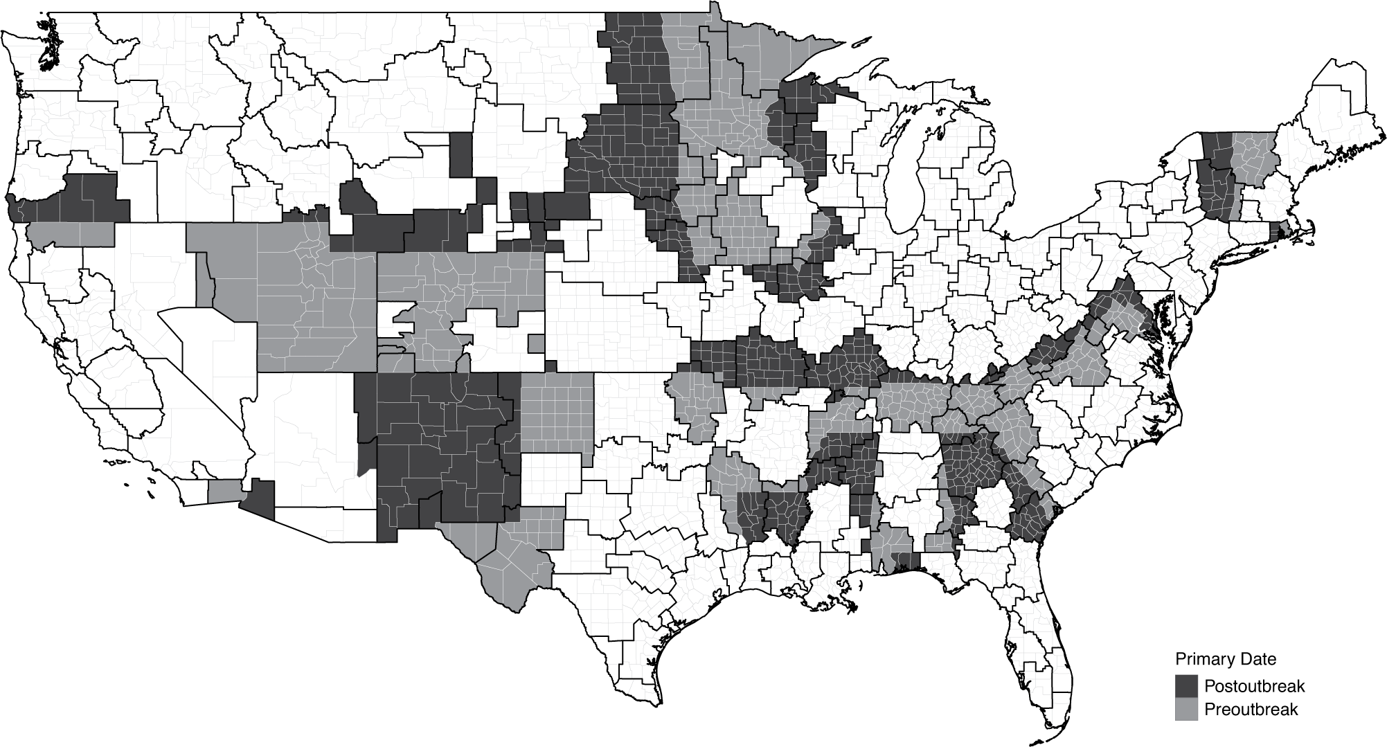
Figure 2. Visually Isolating the Identifying Variation
Note: Counties that share the same DMA but reside in states that voted earlier or later are shaded in gray and black, respectively.
Our second approach reorients our dataset as a panel dataset, recognizing that we only observe each county once. To implement a difference-in-differences estimator, we categorize every county as either exposed or insulated based on the number of cases in their DMA as of March 17th. We calculate the difference in the support for Sanders among these counties that voted prior to March 17th and compare this difference to that measured between exposed and insulated counties that voted on March 17th. The identifying assumption underlying this method is that by differencing out the support for Sanders among counties that would and would not be exposed as of March 17th, we remove any potential selection bias.
We augment this strategy via trajectory-balancing weights (Hazlett and Xu Reference Hazlett and Xu2018), which reweight the control units such that they more closely approximate the treated units based on pretreatment covariates. We balance on the daily number of COVID-19 cases by county, matching all exposed counties that voted on March 17th to those counties that voted prior to March 17th based on the full list of controls given above and their daily exposure to the virus. This approach ensures that we compare an exposed county that voted on March 17th to an as-close-to-identical-as-possible county that voted earlier in terms of its preelection demographic, economic, and social characteristics, as well as a full time-series vector of daily cases through late April 2020. More theoretically, this method means that we are identifying the effect of exposure using the exogeneity of the pandemic as it interacts with the independently determined primary election calendar.
One final concern that we believe grows more problematic as the virus spreads is the stable unit treatment value assumption, or SUTVA. Substantively, this assumption requires that our control counties are not affected by treatment spillovers from treated counties. Our treatment exposure is defined at the DMA level, based on the assumption that the salience of the disease is elevated via local media markets that report on more geographically proximate cases. We believe this is sensible for the beginning of March 2020, when the virus was just beginning to spread across the United States. However, by the end of March, national media outlets (e.g., cable news, newspapers, news websites, and online social media such as Facebook, as discussed in Roose and Dance Reference Roose and Gabriel2020) had shifted coverage to focus almost exclusively on the outbreak as the crisis worsened. Thus many of our notionally “control” counties likely experienced substantial levels of anxiety despite not residing in a DMA with confirmed cases of the virus.
We test the SUTVA assumption by predicting week-by-week variation in two observable behaviors that we believe proxy for anxiety. The first is mobility data that we interpret as a proxy for social distancing behaviors. The second is Google search data for the term “coronavirus.” We show that geographic variation in DMA-level cases is strongly predictive of variation in these proxies in the first three weeks of March but that—in line with violations of SUTVA—exposed and insulated areas show no differences after March 23rd. In addition, we include an exhaustive series of pairwise comparisons in which we define one primary election as treated and another as control in our Supporting Information, which serve as a series of placebo tests for the validity of our identifying variation in first three weeks of March, 2020.
Results
Our first set of results are summarized in Table 1, which presents the coefficient estimates returned by a regression of Sanders two-way vote share (Sanders/Sanders + Biden) on an indicator that takes the value 1 if the county is located in a DMA with one or more confirmed cases of COVID-19 at the election date. The first three columns present the coefficients on exposure to the pandemic using the full data running from February through April. The second three columns subset the data to focus only on the elections that occurred between March 1st and April 7th—the dates after which the pandemic started and before Sanders dropped out of the race. Clustered standard errors at the DMA are presented in parentheses. Columns 1 and 4 present the results of a basic regression using only the controls with DMA fixed effects. Columns 2 and 5 implement the nearest neighbor matching strategy using the Mahalanobis distance (Stuart Reference Stuart2010). Columns 3 and 6 apply weights generated using CBPS (Imai and Ratkovic Reference Imai and Ratkovic2014).
Table 1. Sanders Two-Way Vote Share ∼ Exposure

Note: DMA-cluster robust standard errors in parentheses. The caucus indicator does not have sufficient variation to be included in the March and April subset (columns 4–6). † p < 0.10, *p < 0.05, **p < 0.01, ***p < 0.001.
The results indicate that counties with one or more confirmed cases of the virus in their DMA at the time they went to the polls were significantly less likely to support Sanders than counties without confirmed cases. The coefficients themselves are standard deviations of the two-way vote share for Sanders (1 SD = 14.9 percentage points), suggesting a statistically and substantively significant relationship between exposure and voting behavior, albeit one whose magnitude is exaggerated when we include election results prior to the outbreak. The most conservative estimates generated in the March subset find an effect size of approximately 9 percentage points.
Difference-in-Differences
The preceding results exploit temporal variation in exposure, but operationalize this variation in a cross-sectional regression. In the following section, we instead turn to a difference-in-differences specification in which we compare the difference between exposed and insulated counties prior to the outbreak with the difference in Sanders support among these groups of counties following the outbreak.
The left panel of Figure 3 plots the simple share of the voting age population that supported Sanders among exposed (dark gray) and insulated (light gray) counties prior to (left) and following (right) the outbreak of the virus (defined as beginning on March 10th). These descriptive plots highlight some important patterns in the voters’ response to COVID-19. First, there appears to be a secular decline in support for Sanders among both exposed and insulated counties following the outbreak of the novel coronavirus (left panel). Second, there is some evidence suggesting that the counties that were exposed to the virus and voted after the outbreak shifted more strongly against Sanders than those counties that were not exposed (right panel). These patterns suggest that Sanders enjoyed greater support in areas that were more affected by the virus (younger, more urban areas), but that this support eroded as the virus spread.

Figure 3. Descriptive Differences between Exposed and Insulated Voting Behavior before and after the Outbreak, Defined as Starting on March 10th
Note: The left panel groups counties by whether they were exposed as of March 17th, right panel plots the logged cases as of March 17th by whether the county voted prior to or following the outbreak. Points sized to reflect total turnout.
To test this descriptive intuition, we estimate a difference-in-differences regression of the following form
 $$ \begin{array}{c}{Y}_c={\beta}_0+{\beta}_1{\mathrm{Exp}}_{c, Mar17}+{\beta}_2\unicode{x1D540}\left[\mathrm{Vote}\;\mathrm{Mar}17\right]\\ {}\hskip-2.5pc +{\beta}_3\hskip0.1em \mathrm{Exp}\times \unicode{x1D540}\left[\hskip0.1em \mathrm{Vote}\right]+{\varepsilon}_c\end{array} $$
and plot the marginal effects in Figure 4. As illustrated, there is evidence consistent with the descriptive plots above—counties that were exposed as of March 17th were more supportive of Sanders overall, but they were significantly more supportive when they voted prior to March 17th. The interaction coefficient on this specification is statistically significant and of commensurate magnitude to that presented in Table 1 (estimate = −6.97 percentage points; SE = 2.15).

Figure 4. Marginal Effects Plot of the Difference-in-Differences Results
Note: Coefficients in the preperiod capture the difference between exposed and insulated counties as of March 17 but that voted prior to March 17th. Coefficients in the post period reflect the difference in exposed and insulated counties that voted on March 17th.
To confirm the sensitivity of the difference-in-differences finding to the choice of outbreak date, we regress support for Sanders on exposure week by week and plot these coefficients in Figure 5. As illustrated, there is clear evidence of a positive relationship between exposure as of March 17th and support for Sanders up until March 10th. On March 17th, we see a significant negative relationship when weighting counties using CBPS.

Figure 5. Week-by-Week Regressions of Sanders’s Two-Way Vote Share on a Dummy Indicator for Whether the County Was Exposed to the Virus on March 17th
Note: Lighter points and bars are coefficients estimated using the basic regression including all controls. Darker points and bars are coefficients estimated applying the CBPS weights to balance exposed and insulated counties.
These plots are not meant to support well-identified inferential conclusions, although the correlations we document consistently point toward support for Sanders slipping in exposed areas that we would otherwise expect to be quite supportive. These plots do clarify the sources of identifying variation we rely on in the results that follow. Specifically, by comparing counties based on their number of cases as of March 17th and dividing them into groups that voted prior to that date and those that voted on March 17th, we emphasize the selection problems in this exercise. There is clear evidence that areas more affected by the pandemic were also those more naturally inclined to support Sanders. The goal therefore is to reweight the data to provide the most appropriate counterfactual for our notionally “treated” counties that (1) had cases and (2) voted on March 17th.
To do so we turn to trajectory balancing, a method that reweights control units to appear as similar to treated groups as possible over the entire pretreatment period (Hazlett and Xu Reference Hazlett and Xu2018). We use a jackknife approach in which we drop one exposed county at a time, reestimate the trajectory balancing weights, and calculate the difference in Sanders’s two-way vote share between exposed and weighted control counties. We repeat this process three times, corresponding to the March election dates of March 3rd, March 10th, and March 17th, and we plot the estimates as densities in Figure 6. Again we see evidence suggesting that exposed counties were insignificantly more supportive of Sanders as of March 3rd, as compared with otherwise similar counties that voted in February. However, by March 10th and then most strikingly by March 17th, this relationship is reversed. Substantively, these results suggest that counties that voted on March 17th and were located in a DMA with at least one confirmed COVID-19 case were approximately 15 percentage points less supportive of Sanders on average than similar counties that voted prior to March 17th, commensurate to the coefficients estimated in the baseline naive regressions in Table 1.
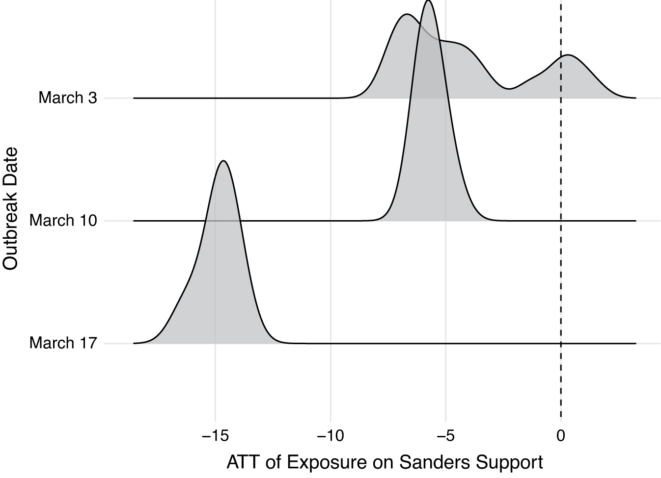
Figure 6. Jackknife Estimates
Note: The values were generated by dropping each exposed county one at a time, estimating the trajectory-balancing weights, and then calculating the difference between the exposed support for Sanders and the weighted control support. The y-axis indicates whether we compare exposed counties that voted on March 3rd, March 10th, or March 17th.
Mechanisms: The Spread of Anxiety
The results summarized above are consistent with our theorized flight-to-safety mechanism in which the COVID-19 pandemic alters the relative appeal of mainstream and antiestablishment candidates. The methods employed above combine the exogeneity of the pandemic with the orthogonal primary election dates, in so doing endeavoring to purge our estimates of confounding selection effects.
Our theorized mechanism rests on the assumption that differences in the exposure to the pandemic cause differences in anxiety, which then generate differences in observed vote shares for Sanders. To test whether anxiety is in fact responding to the outbreak, we predict daily cross-sectional variation in Google searches about the virus. We view increased interest in the virus represented by Google search data is a proxy for increased anxiety about its health risks. We obtain these measures at the DMA level daily from December 30th, 2019, to April 30th, 2020.
In Figure 7, we show that search traffic is significantly correlated with DMA-level variation in cases, particularly in the week following Super Tuesday. The top words that were associated with searches for “coronavirus” are displayed above the coefficients. As illustrated, not only are those living in exposed areas more likely to search for “coronavirus” than those living in unexposed areas; they are also pairing their search terms with other anxiety-associated words. These plots provide growing evidence of “saturation” over time in the sense that geographic heterogeneity is no longer meaningful when everyone is equally anxious. Specifically, we note that the significant positive relationship between Google searches for “coronavirus” and DMA-level cases disappears after March 10th, meaning that the search profile in areas with many cases was no different from the search profile in areas with few cases. These patterns suggest that COVID-induced anxiety becomes so widespread by mid-March that we are no longer able to use geographic variation to identify the effect of the pandemic.Footnote 19

Figure 7. Daily (x-axis) Coefficients (y-axis) on the Relationship between DMA-Level Cases and DMA-Level Google Searches for “Coronavirus,” Including State Random Effects
Note: Vertical dashed bars indicate primary dates. Top three related search phrases given above each bar.
Considering Alternative Explanations
It is possible that it is not anxiety that induces the shift toward Biden but either differences in turnout, which covary with anxiety, or a concurrent “party-decides” phenomenon. In the Supporting Information, we explore these dynamics, finding no support for the notion that they explain the empirical patterns we observe.
First, we look for evidence of an alternative pathway in which the pandemic’s differential suppression of turnout drives the results. There are two versions of this alternative story. The first focuses on the differences in health risks by age and posits that those most threatened by exposure might be less likely to turn out. If this group is also more likely to support Sanders, it would suggest an alternative explanation for the effects we document. (Of course, Sanders’s popularity among young voters is well documented, while the elderly are most threatened by the virus.) Nevertheless, we look for differences in turnout by county age demographics and find little support for this alternative turnout explanation.
The second turnout story is that the Sanders campaign was effectively finished after Biden’s convincing victory in South Carolina on February 29th. In this scenario, a number of would-be Sanders voters were planning on casting what were effectively protest votes, and those in COVID-exposed areas didn’t bother since the “costs” of doing so were higher. If this were the case, we should expect to see a decline in turnout in more pro-Sanders counties following the South Carolina primary. Again, we test this claim in our Supporting Information, finding little evidence to support it.
We additionally consider whether our results might be spuriously driven by a “party-consolidation” effect. This concern is motivated by the theory that “the Party Decides”—that is, the possibility that party elites hold decisive power over the candidate selection process (Cohen et al. Reference Cohen, Karol, Noel and Zaller2009), these elites exercised their power in favor of Biden, and these elites did so just as the pandemic was spreading. If the Democratic Party decided to back Biden just as COVID-19 spread across the country, it might appear that the virus caused Sanders’s decline when it was actually mere coincidence. This concern is somewhat mitigated by the observation that not only would the party-decides explanation have to occur at the same time as the outbreak; it would also have to be correlated with the pandemic’s geographic distribution to account for our results. Furthermore, to the extent that the Democratic Party did “decide” on Biden, it arguably did so prior to Super Tuesday, meaning that its effect would be that of influencing primary vote shares in both the pre and post periods of the difference-in-differences analyses.Footnote 20 Nevertheless, we test this alternative explanation using a variety of placebo tests in the Supporting Information including a permutation test in which we break the geographic distribution of the outbreak and examine whether the temporal variation still predicts a decline in Sanders’s support (it doesn’t), all alternative assignments of vote dates to treated and control conditions, and tests of whether more anti-Sanders areas were more exposed to COVID-19 (they weren’t).
Survey Experimental Evidence
Even with the exhaustive checks on our main results summarized above and in our Supporting Information, convincingly identifying our theory is a challenge using observational data. There are a number of differences between any two candidates that might explain differential reactions to them in light of the pandemic. In order to isolate the anxiety mechanism, we fielded a survey experiment on Amazon’s Mechanical Turk platform between May 14th and May 20th, 2020, in which we randomly assigned respondents to read a summary of a potential future course for the pandemic and then choose between two hypothetical challengers for executive office. We randomly assigned respondents to read either an optimistic assessment of the pandemic (anxiety-relieving) or a pessimistic assessment (anxiety-inducing), both of which were based on real media accounts and expert assessments as of May 10th, 2020. The optimistic assessment highlighted the progress made toward creating a vaccine, the potential use of existing drugs to combat the virus, and statistical evidence suggesting that most of the country had the worst part of the pandemic behind them. The pessimistic assessment painted a bleak picture of the possibility of a second wave of infections and a longer wait before vaccines became available, and it suggested that existing reports likely undercounted the number of cases and deaths to date.Footnote 21
We randomly varied the candidates along four dimensions: age (45 or 48), occupation (accountant or lawyer), education (law school or local college), policy platform (health care or education), and—our primary object of interest—antiestablishment or mainstream candidate. The antiestablishment candidate was described as an individual who “seeks fundamental transformation of the economic, social, and political order. He believes that the system is broken, and the time for radical change is now.” The mainstream candidate was described as an individual who “believes in strengthening existing economic, social, and political institutions. He believes that we must come together and reinvest in our system, strengthening its foundations to support generations to come.”
Our main quantity of interest is whether exposure to the pessimistic treatment reduced support for the antiestablishment candidate, corresponding to our theorized flight-to-safety mechanism. Table 2 illustrates the results, finding that reading a pessimistic description of the pandemic reduces support for the antiestablishment candidate, in line with our theoretical intuition.
Table 2. Survey Experiment Results

Note: Robust standard errors presented in parentheses. Anxiety prime emphasizes the possibility of a second wave of infections and a longer wait before vaccines become available, and it suggested that existing reports likely undercounted the number of cases and deaths. The “Attentive” subset are those who spent more than three minutes completing our short survey. † p < 0.10, *p < 0.05, **p < 0.01, ***p < 0.001.
We also find that these relationships dominate even when we randomly vary the policy platform adopted by our hypothetical candidates. Specifically, the increased preference for the mainstream candidate holds even when the comparison is with an antiestablishment candidate running on a platform centered on health care reform. Any variation in other qualities (e.g., leadership or executive experience) that may be inferred from the different occupations or educational histories of our candidates is randomly assigned and in any case has no detectable effect on voting intent. Furthermore, the experimental setting is about two hypothetical challengers running for executive office, controlling for the potential strategic voting behavior of a primary setting (Abramson et al. Reference Abramson, Aldrich, Paolino and Rohde1992). Therefore, we interpret these results as a direct test of mainstream versus antiestablishment preference in response to anxiety that obtains independent of specific candidate qualities such as leadership or strategic assessments of candidate electability in a general election.
Generalizability
Our analysis thus far combines observational evidence from the 2020 Democratic primaries with a survey experiment fielded among US-based respondents. Our findings consistently support our argument that voters exhibit a flight to safety during periods of heightened anxiety. However, does the effect generalize to other offices? And is there evidence that a flight to safety operates outside of the US?
To address these questions, we conduct two additional observational studies. The first looks at primary elections for members of the House of Representatives in 2020 to show that more extreme candidates suffered in states with later elections and in congressional districts with greater exposure to the pandemic. The second looks at 2020 French municipal elections to demonstrate that similar patterns obtain in contexts outside the United States.
US House Primaries
We classify a candidate for a House seat as “extreme” if they are endorsed either by the Justice Democrats movement (an antiestablishment leftist coalition) or by the Tea Party movement (an antiestablishment rightist coalition), yielding eight Democratic Party candidates and 62 Republican party candidates that we consider antiestablishment. We estimate an interacted specification in which we predict the candidate’s electoral support as a function of whether they are an extreme candidate, the number of COVID-19 cases or deaths in their Congressional District, and the interaction. Formally,
 $$ \begin{array}{c}{y}_{c,d}={\gamma}_d+{\beta}_1 anti\hbox{-}{estab}_c+{\beta}_2{covid}_d\\ {}\hskip2pc +\hskip.2pc {\beta}_3 anti\hbox{-} estab\times covid+{\varepsilon}_{c,d},\end{array} $$
where subscripts d represent Congressional Districts and c indicates the candidates. We include district fixed effects and cluster standard errors at the district. The results, summarized in Table 3, indicate that antiestablishment candidates received less support at the ballot box in areas more exposed to the pandemic, as seen by the negative and statistically significant interaction terms. These patterns hold whether we predict variation in their contest-specific vote share or the logged votes they received after controlling for total votes cast. The patterns also obtain when we replace the logged COVID-19 cases predictor with logged deaths, although they are weaker.Footnote 22
Table 3. Antiestablishment Vote Share as a Function of COVID-19 Exposure

Note: District-cluster robust standard errors presented in parentheses. † p < 0.10, *p < 0.05, **p < 0.01, ***p < 0.001.
2020 French Municipal Elections
We conclude our analysis by testing whether a similar pattern holds outside of the United States. We obtain department-level data on COVID-19 cases in France, which we match with election returns from the two-wave municipal election cycle of 2020. These elections occurred in two waves in the first half of 2020, first on March 15th just prior to the widespread outbreak of the pandemic and again on June 28th.Footnote 23 We consider all centrist parties (LREM, LMDM, LUDI, LUC, LDVC), as well as the largest parties on the center-left (LSOC) and center-right (LRR), mainstream parties. We plot the descriptive change in electoral fortunes of these parties between March and June in Figure 8, highlighting the electoral penalty suffered by less mainstream parties. These descriptive patterns are highly statistically significant in a difference-in-differences specification in which we interact mainstream status with election wave, suggesting an almost 10-percentage-point shift in relative electoral fortunes (results included in the Supporting Information). There is also evidence of greater effects where COVID was more widespread, suggesting both temporal and geographic heterogeneity consistent with our other findings.

Figure 8. Descriptive Evidence from France
Note: Mainstream parties benefited (gray) and nonmainstream parties lost (black) between the March and June municipal-level elections. Left panel plots average aggregate vote share (y-axis) by party (shaded bars) and period (x-axis). Right panel plots average aggregate vote share (y-axis) by logged COVID-19 deaths (x-axis) and party (shaded points).
Discussion
In this paper, we build on a rich literature to develop a general understanding of how anxiety influences vote choice. Our framework—which we refer to as a political flight to safety—predicts that shocks to voter anxiety improve the electoral chances of mainstream candidates.
We provide evidence of our claim across four empirical contexts related to COVID-19. Our main analysis describes a causal effect of the pandemic on Bernie Sanders’s declining fortunes in the Democratic primary election of 2020. We supplement this result with similar evidence in the House of Representatives, in which antiestablishment candidates disproportionately lost where exposure to the virus was greater. We also show that this pattern travels outside of the US, finding that less-mainstream parties in French municipal elections were penalized at the ballot box between the first (March 2020) and second (June 2020) rounds of voting. Finally, we fielded a survey experiment in which we experimentally manipulated the anxiety-inducing qualities of a prime about COVID-19, before asking respondents to indicate their preference for a more mainstream or more antiestablishment candidate. Across all contexts, we find consistent evidence that anxiety prompts a preference for the status quo regardless of other attributes including policy positions, experience, and office.
The magnitude of the effects we summarize are nontrivial, ranging from a 2-percentage-point penalty against antiestablishment candidates for the House of Representatives, to 7 percentage points in our survey experiment, to 10 percentage points in French municipal elections, to between 7 and 15 percentage points in the Democratic primary election between Bernie Sanders and Joe Biden. These effect sizes are substantially larger than those from existing work on political campaigns themselves, where coefficient magnitudes greater than 1 percentage point are rare (Kalla and Broockman Reference Kalla and Broockman2018).
There are some reasons to believe we capture an unusually large treatment “dosage” for our underlying anxiety mechanism in the sense that COVID-19 is a particularly large shock. Future research might explore the extent to which other sources of anxiety induce a political flight to safety and the magnitude of the flight to safety these sources produce. Further work might also explore whether the flight to safety is conditioned by, among other factors, the closeness of elections and thus the likelihood that an antiestablishment candidate—itself a potential source of anxiety for some voters—might actually be elected.
Our intuition accommodates existing research documenting a positive relationship between anxiety and voter preference for leadership (Merolla and Zechmeister Reference Merolla and Zechmeister2009), protection (Albertson and Gadarian Reference Albertson and Gadarian2015), and conservativism (Stenner Reference Stenner2005). However, a political flight to safety is at once both more general and more precise. While it operates through the valence (rather than policy preference) component of voters’ utility functions, it is neither a specific candidate quality such as leadership or experience that is rewarded nor a directional right-wing preference that is activated. Building on existing theory, this paper provides evidence that the flight to safety operates even where there is no incumbent and where retrospective evaluations do not influence voter behavior. A broad valence preference for the safety of the familiar is intensified by voters’ anxiety—a preference that is always present but receives more weight under conditions of anxiety. In this sense, our framework connects with work on system justification that predicts that even those disadvantaged under the status quo will defend it in order to reduce uncertainty, particularly when anxiety is higher (Jost et al. Reference Jost, Glaser, Kruglanski and Sulloway2003; Van der Toorn et al. Reference Van der Toorn, Feinberg, Jost, Kay, Tyler, Willer and Wilmuth2015).
The implications of voters’ anxiety-induced preference for the status quo are far-reaching, particularly if the political strength of radical movements is itself a source of public anxiety. A political flight to safety may operate as a brake on radical change, carrying provocative implications for antiestablishment candidates, parties, and even democratic accountability. We leave these extensions to future research. What this paper can say with confidence is that, as it does in financial markets, anxiety prompts a flight to safety in the market for political candidates.
Supplementary Materials
To view supplementary material for this article, please visit http://dx.doi.org/10.1017/S0003055421000691.
DATA AVAILABILITY STATEMENT
Research documentation and data that support the findings of this study are openly available at the American Political Science Review Dataverse: https://doi.org/10.7910/DVN/S5YMS7.
ACKNOWLEDGMENTS
We would like to thank Bjorn Bremer, Filipe Campante, Charlotte Cavaille, Alex Coppock, Drew Dimmery, Christina Eder, Patrick Egan, Timon Forster, Erik Jones, Robert Kubenick, Matthias Mathijs, David Steinberg, and Ryan Welzeus for their help in locating data and in commenting on earlier drafts. Special thanks to Ben Lauderdale for his guidance in shaping this paper from the research note it began as and to the Journal of COVID Economics for publishing a preprint of that note. Dan additionally would like to thank Johns Hopkins SAIS, Dakar’s West Africa Research Center and Leiden University’s Institute of Political Science, where he was a visitor for much of the initial drafting (Dakar) and subsequent revision (Leiden) of this work.
FUNDING STATEMENT
This research was partially funded by the Niehaus Center for Globalization and Governance, Princeton University.
CONFLICT OF INTEREST
The authors declare no ethical issues or conflicts of interest in this research.
ETHICAL STANDARDS
The authors declare the human subjects research in this article was deemed exempt from review by the Princeton IRB board (IRB #12870).


Comments
No Comments have been published for this article.