


Introduction
Competitive elections create a system whereby voters can hold policy makers accountable for their actions. This mechanism should make politicians hesitant to engage in malfeasance such as blatant acts of corruption. Increases in public information regarding corruption should therefore decrease levels of corruption in government, as voters armed with information expel corrupt politicians (Kolstad and Wiig Reference Kolstad and Wiig2009; Rose-Ackerman and Palifka Reference Rose-Ackerman and Palifka2016). However, this theoretical prediction is undermined by the observation that well-informed voters continue to vote corrupt politicians into office in many democracies.
Political scientists and economists have therefore turned to experimental methods to test the causal effect of learning about politician corruption on vote choice. Numerous experiments have examined whether providing voters with information about the corrupt acts of politicians decreases their re-election rates. These papers often suggest that there is little consensus on how voters respond to information about corrupt politicians (Arias et al. Reference Arias, Larreguy, Marshall and Querubin2018; Botero et al. Reference Botero, Cornejo, Gamboa, Pavao and Nickerson2015; Buntaine et al. Reference Buntaine, Jablonski, Nielson and Pickering2018; De Vries and Solaz Reference De Vries and Solaz2017; Klašnja, Lupu, and Tucker Reference Klašnja, Lupu and Tucker2017; Solaz, De Vries, and de Geus Reference Solaz, De Vries and de Geus2019). Others indicate that experiments have provided us with evidence that voters strongly punish individual politicians involved in malfeasance (Chong et al. Reference Chong, De La O, Karlan and Wantchekon2014; Weitz-Shapiro and Winters Reference Weitz-Shapiro and Winters2017; Winters and Weitz-Shapiro Reference Winters and Weitz-Shapiro2015, Reference Winters and Weitz-Shapiro2016).
By contrast, meta-analysis suggests that: (1) in aggregate, the effect of providing information about incumbent corruption on incumbent vote share in field experiments is approximately zero, and (2) corrupt candidates are punished by respondents by approximately 32 percentage points across survey experiments. This suggests that survey experiments may provide point estimates that are not representative of real-world voting behavior. Field experimental estimates may also not recover the “true” effects due to design decisions and limitations.
I also examine mechanisms that may give rise to this discrepancy. I do not find systematic evidence of publication bias. I discuss the possibility that social desirability bias may lead survey respondents to under-report socially undesirable behavior. The costs of changing one’s vote are also lower and more abstract in hypothetical environments. In field experiments, the magnitude of treatment effects may be small due to weak treatments and noncompliance. Field and survey experiments also may be measuring different causal estimands due to differences in context and survey design. Finally, surveys may not capture the complexity and costliness of real-world voting decisions. Conjoint experiments attempt to alleviate some of these issues, but they are often analyzed in ways that may fail to illuminate the most substantively important comparisons. I suggest examining the probability of voting for candidates with specific combinations of attributes in conjoint experiments when researchers have priors about the conditions that shape voter decision-making and using classification trees to illuminate these conditions when they do not.
I therefore (1) find that the “true” or average effect of voter punishment of revealed corruption remains unclear, but it is likely to be small in magnitude in actual elections, (2) show that researchers should use caution when interpreting point estimates in survey experiments as indicative of real-world behavior, (3) explore methodological reasons that estimates may be particularly large in surveys and small in field experiments, and (4) offer suggestions for the design and analysis of future experiments.
Corruption Information and Electoral Accountability
Experimental support for the hypothesis that providing voters with information about politicians’ corrupt acts decreases their re-election rates is mixed. Field experiments have provided some causal evidence that informing voters of candidate corruption has negative (but generally small) effects on candidate vote share. This information has been provided by randomized financial audits (Ferraz and Finan Reference Ferraz and Finan2008), fliers revealing corrupt actions of politicians (Chong et al. Reference Chong, De La O, Karlan and Wantchekon2014; De Figueiredo, Hidalgo, and Kasahara Reference De Figueiredo, Hidalgo and Kasahara2011), and SMS messages (Buntaine et al. Reference Buntaine, Jablonski, Nielson and Pickering2018). However, near-zero and null findings are also prevalent, and the negative and significant effects reported above sometimes only manifest in particular subgroups. Banerjee et al. (Reference Banerjee, Green, Green and Pande2010) primed voters in rural India not to vote for corrupt candidates, and Banerjee et al. (Reference Banerjee, Kumar, Pande and Felix2011) provided information on politicians’ asset accumulation and criminality, with both studies finding near-zero and null effects on vote share. Boas, Hidalgo, and Melo (Reference Boas, Daniel Hidalgo and Melo2019) similarly find zero and null effects from distributing fliers in Brazil. Finally, Arias et al. (Reference Arias, Larreguy, Marshall and Querubin2018) and Arias et al. (Reference Arias, Balán, Larreguy, Marshall and Querubín2019) find that providing Mexican voters with information (fliers) about mayoral corruption actually increased incumbent party vote share by 3%.Footnote 1
By contrast, survey experiments consistently show large negative effects from informational treatments on vote share for hypothetical candidates. These experiments often manipulate moderating factors other than information provision (e.g., quality of information, source of information, partisanship, whether corruption brings economic benefits to constituents, etc.), but even so, they systematically show negative treatment effects (Anduiza, Gallego, and Muñoz Reference Anduiza, Gallego and Muñoz2013; Avenburg Reference Avenburg2019; Banerjee et al. Reference Banerjee, Green, McManus and Pande2014; Boas, Hidalgo, and Melo Reference Boas, Daniel Hidalgo and Melo2019; Breitenstein, Reference Breitenstein2019; Eggers, Vivyan, and Wagner Reference Eggers, Vivyan and Wagner2018; Franchino and Zucchini Reference Franchino and Zucchini2015; Klašnja and Tucker Reference Klašnja and Tucker2013; Klašnja, Lupu, and Tucker Reference Klašnja, Lupu and Tucker2017; Mares and Visconti Reference Mares and Visconti2019; Vera Reference Vera2019; Weitz-Shapiro and Winters Reference Weitz-Shapiro and Winters2017; Winters and Weitz-Shapiro Reference Winters and Weitz-Shapiro2013, Reference Winters and Weitz-Shapiro2015, Reference Winters and Weitz-Shapiro2016, Reference Winters and Weitz-Shapiro2020). These experiments have historically taken the form of single treatment arm or multiple arm factorial vignettes, but more recently have tended toward conjoint experiments (Agerberg Reference Agerberg2020; Breitenstein Reference Breitenstein2019; Chauchard, Klašnja, and Harish Reference Chauchard, Klašnja and Harish2019; Franchino and Zucchini Reference Franchino and Zucchini2015; Klašnja, Lupu, and Tucker Reference Klašnja, Lupu and Tucker2017; Mares and Visconti Reference Mares and Visconti2019).
Boas, Hidalgo, and Melo (Reference Boas, Daniel Hidalgo and Melo2019) find differential results in a pair of field and survey experiments conducted in Brazil—zero and null in the field but large, negative, and significant in the survey. They argue that norms against malfeasance in Brazil are constrained by other factors at the polls but that “differences in research design are unlikely to account for much of the difference in effect size” (10).Footnote 2 Boas, Hidalgo, and Melo (Reference Boas, Daniel Hidalgo and Melo2019) identify moderating factors specific to Brazil—low salience of corruption to voters in municipal elections and the strong effects of dynastic politics—to explain the small effects in their field experiment. However, meta-analysis demonstrates that this discrepancy exists not only in Boas, Hidalgo, and Melo’s experiments in Brazil but extends across a systematic review of all countries and studies conducted to date. This suggests that the discrepancy between field and survey experimental findings is driven by methodological differences, rather than Brazil-specific features. I therefore enumerate features inherent in the research designs of field and survey experiments that may drive the small effects in field experiments and large effects in survey experiments.
Lab experiments that reveal corrupt actions of politicians to fellow players and then measure vote choice also show large negative treatment effects. While recognizing that the sample size of studies is extremely small, a meta-analysis of the three lab experiments that meet this study’s selection criteria reveal a point estimate of approximately -33 percentage points (Arvate and Mittlaender Reference Arvate and Mittlaender2017; Azfar and Nelson Reference Azfar and Nelson2007; Solaz, De Vries, and de Geus Reference Solaz, De Vries and de Geus2019) (see Online Appendix Figure A.1).Footnote 3 This discrepancy is worth noting, as previous examinations of lab–field correspondence have found evidence of general replicability (Camerer Reference Camerer2011; Coppock and Green Reference Coppock and Green2015).
Research Design and Methods
Selection Criteria
I followed standard practices to locate the experiments included in the meta-analysis. This included following citation chains and searches of data bases using a variety of relevant terms (“corruption experiment,” “corruption field experiment,” “corruption survey experiment,” “corruption factorial,” “corruption candidate choice,” “corruption conjoint,” “corruption, vote, experiment,” and “corruption vignette”). Papers from any discipline are eligible for inclusion, but in practice stem only from economics and political science. Both published articles and working papers are included so as to ensure the meta-analysis is not biased towards published results. In total, I located 10 field experiments from 8 papers, and 18 survey experiments from 15 papers.
Field experiments are included if researchers randomly assigned information regarding incumbent corruption to voters then measured corresponding voting outcomes. This therefore excludes experiments that randomly assign corruption information but use favorability ratings or other metrics rather than actual vote share as their dependent variable. I include one natural experiment, Ferraz and Finan (Reference Ferraz and Finan2008), as random assignment was conducted by the Brazilian government. Effects reported in the meta-analysis come from information treatments on the entire sample of study only, not subgroup or interactive effects that reveal the largest treatment effects.
For survey experiments, studies must test a no-information or clean control group versus a corruption information treatment group and measure vote choice for a hypothetical candidate. This necessarily excludes studies that compare one type of information provision (e.g., source) with another and the control group is one type of information rather than no information or where the politician is always known to be corrupt (Anduiza, Gallego, and Muñoz Reference Anduiza, Gallego and Muñoz2013; Botero et al. Reference Botero, Cornejo, Gamboa, Pavao and Nickerson2015; Konstantinidis and Xezonakis Reference Konstantinidis and Xezonakis2013; Muñoz, Anduiza, and Gallego Reference Muñoz, Anduiza and Gallego2012; Rundquist, Strom, and Peters Reference Rundquist, Strom and Peters1977; Weschle Reference Weschle2016). In many cases, studies have multiple corruption treatments (e.g., high quality information vs. low quality information, co-partisan vs. opposition party, etc.). In these cases, I replicate the studies and code corruption as a binary treatment (0 = clean, 1 = corrupt) where all treatment arms that provide corruption information are combined into a single treatment. Studies that use non-binary vote choices are rescaled into a binary vote choice.Footnote 4
Included Studies
A list of all papers—disaggregated by field and survey experiments—that meet the criteria outlined above are provided in Table 1 and Table 2. A list of lab experiments (four total) can also be found in the Online Appendix Table A.1, although these studies are not included in the meta-analysis. A list of excluded studies with justification for their exclusion can be found in the Online Appendix Table A.2.
Table 1. Field Experiments

Table 2. Survey Experiments

Additional Selection Comments
Additional justification for the inclusion or exclusion of certain studies as well as coding and/or replication choices may be warranted in some cases. Despite often being considered a form of corruption (Rose-Ackerman and Palifka Reference Rose-Ackerman and Palifka2016), I exclude electoral fraud experiments, as whether vote buying constitutes clientelism or corruption is a matter of debate (Stokes et al. Reference Stokes, Dunning, Nazareno and Brusco2013). The field experiment conducted by Banerjee et al. (Reference Banerjee, Green, Green and Pande2010) is included. However, the authors treated voters with a campaign not to vote for corrupt candidates in general, but they did not provide voters with information on which candidates were corrupt. Similarly, the field experiment conducted by Banerjee et al. (Reference Banerjee, Kumar, Pande and Felix2011) is included, but their treatment provided information on politicians’ asset accumulation and criminality, which may imply corruption but is not as direct as other types of information provision. The point estimates remain approximately zero when these studies are excluded from the meta-analysis (see Online Appendix Figure A.2 and Table A.6).
With respect to survey experiments, Chauchard, Klašnja, and Harish (Reference Chauchard, Klašnja and Harish2019) include two treatments—wealth accumulation and whether the wealth accumulation was illegal. The effect reported here is the illegal treatment only. This is likely a conservative estimate, as the true effect is a combination of illegality and wealth accumulation. Winters and Weitz-Shapiro (Reference Winters and Weitz-Shapiro2016) and Weitz-Shapiro and Winters (Reference Weitz-Shapiro and Winters2017) report results from the same survey experiment, as do Winters and Weitz-Shapiro (Reference Winters and Weitz-Shapiro2013) and Winters and Weitz-Shapiro (Reference Winters and Weitz-Shapiro2015). Therefore, the results for each of these are only reported once. The survey experiment in De Figueiredo, Hidalgo, and Kasahara (Reference De Figueiredo, Hidalgo and Kasahara2011) is excluded from the analysis because it does not use hypothetical candidates, but instead it asks voters if they would have changed their actual voting behavior in response to receiving corruption information. This study has a slightly positive and null finding. Including this study, the point estimates are 32 and 31 percentage points using fixed and random effects estimation, respectively (see Online Appendix Figure A.3 and Table A.9).
Results
Survey experiments estimate much larger negative treatment effects of providing information about corruption to voters relative to field experiments. In fact, the field-experimental results in Figure 1 reveal a precisely estimated point estimate of approximately zero and suggest that we cannot reject the null hypothesis of no treatment effect (the 95% confidence interval is -0.56 to 0.15 percentage points using fixed effects and -2.1 to 1.4 using random effects). By contrast, Figure 2 shows that corrupt candidates are punished by respondents by approximately 32 percentage points in survey experiments based on fixed and random effects meta-analysis (the 95% confidence interval is -32.6 to -31.2 percentage points using fixed effects and -38.2 to -26.2 using random effects). Of the 18 survey experiments, only one shows a null effect (Klašnja and Tucker Reference Klašnja and Tucker2013), while all others are negative and significantly different from zero at conventional levels.

Figure 1. Field Experiments: Average Treatment Effect of Corruption Information on Incumbent Vote Share and 95% Confidence Intervals
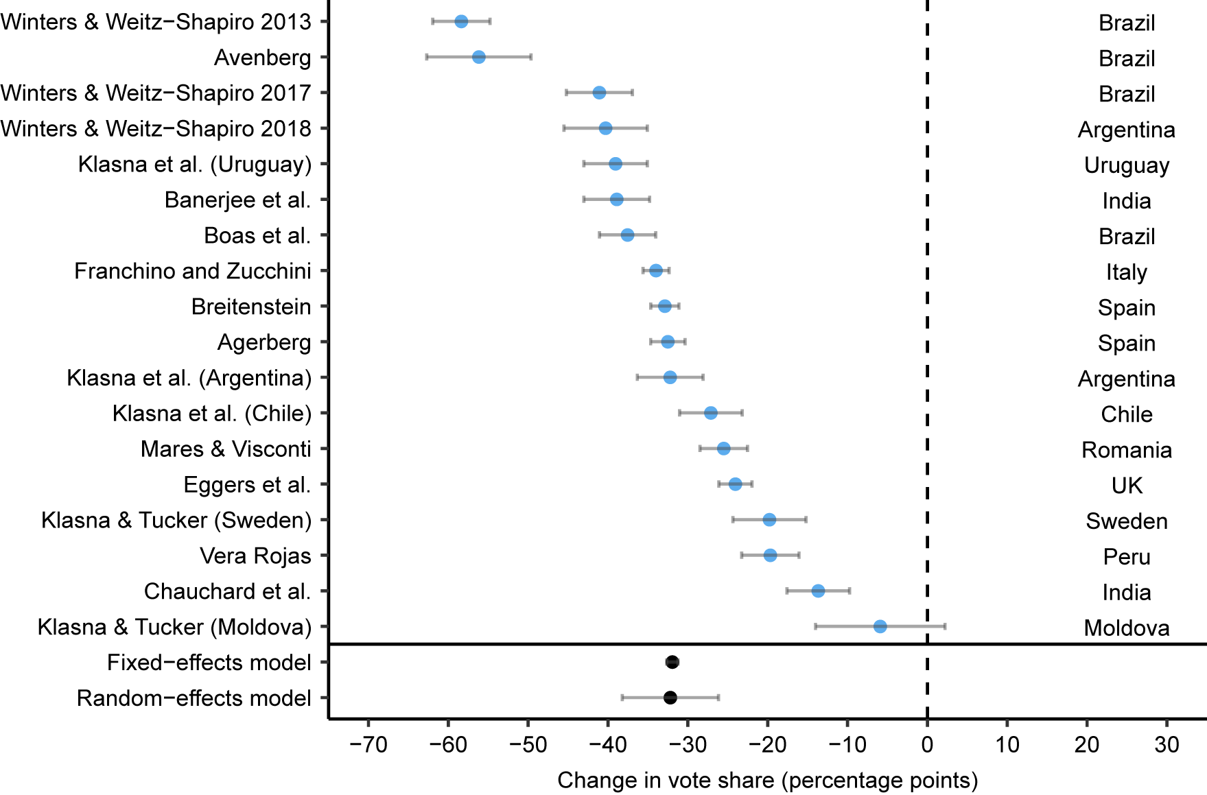
Figure 2. Survey Experiments: Average Treatment Effect of Corruption Information on Incumbent Vote Share and 95% Confidence Intervals
Examining all studies together, a test for heterogeneity by type of experiment (field or survey) reveals that up to 68% of the total heterogeneity across studies can be accounted for by a dummy variable for type of experiment (0 = field, 1 = survey) (see Online Appendix Table A.5). This dummy variable has a significant association with the effectiveness of the information treatment at the 1% level. In fact, with this dummy variable included, the overall estimate across studies is -0.007, while the point estimate of the survey dummy is -0.315.Footnote 5 This implies that the predicted treatment effect across experiments is not significantly different from zero when an indicator for type of experiment is included in the model. In other words, the majority of the heterogeneity in findings is accounted for by the type of experiment conducted.
Exploring the Discrepancy
What accounts for the large difference in treatment effects between field and survey experiments? One possibility is publication bias. Null results may be less likely to be published than significant results, particularly in a survey setting. A second possibility is social desirability bias, which may cause respondents to under-report socially undesirable behavior. Related is hypothetical bias, in which costs are more abstract in hypothetical environments. Survey and field experiments may also not mirror each other and/or real-world voting decisions. Potential ways in which the survey setting may differ from the field are: treatment salience and noncompliance, differences in outcome choices, and costliness/decision complexity. Weak treatments and noncompliance may decrease treatment effect sizes in field experiments. Design decisions may change the choice sets available to respondents. Finally, surveys may not capture the complexity and costliness of real-world voting decisions. It is possible that more complex factorial designs—such as conjoint experiments—may more successfully approximate real-world settings. However, common methods of analysis of conjoint experiments may not capture all theoretical quantities of interest.
Publication Bias and P-Hacking
Publication bias and p-hacking can lead to overestimated effects in meta-analysis (Carter et al. Reference Carter, Schönbrodt, Gervais and Hilgard2019; Duval and Tweedie Reference Duval and Tweedie2000; Sterne, Egger, and Smith Reference Sterne, Egger and Smith2001; van Aert, Wicherts, and van Assen Reference Van Aert, Wicherts and van Assen2019). While I have identified heterogeneity stemming from the type of experiment performed as a potential source of overestimation, this may reflect that null results are less likely to be published than studies with large and significant negative treatment effects. I therefore now turn to the possibility of publication bias and/or p-hacking. To formally test for publication bias, I use the p-curve, examination of funnel plot asymmetry, trim and fill, and PET-PEESEFootnote 6 methods.Footnote 7
Of the eight field experimental papers located, only five are published. By contrast, only one of the 15 survey experimental papers remains unpublished, and this is a recent draft. This may reflect that the null results from field experiments are less likely to be published than their survey counterparts with large and highly significant negative treatment effects. While recognizing that the sample size of studies is small, OLS and logistic regression do not indicate that reported p-value is a significant predictor of publication status, although the directionality of coefficients is consistent with lower p-values being more likely to be published (see Online Appendix Table A.11). However, this simple analysis is complicated by the fact that the p-value associated with the average treatment effect across all subjects may not be the primary p-value of interest in the paper.
To more formally test for publication bias, I first use the p-curve (Simonsohn, Nelson, and Simmons Reference Simonsohn, Nelson and Simmons2014a, Reference Simonsohn, Nelson and Simmons2014b; Simonsohn, Simmons, and Nelson Reference Simonsohn, Simmons and Nelson2015). The p-curve is based on the premise that only “significant” results are typically published, and it depicts the distribution of statistically significant p-values for a set of published studies. The shape of the p-curve is indicative of whether or not the results of a set of studies are derived from true effects, or from publication bias. If p-values are clustered around 0.05 (i.e., the p-curve is left skewed), this may be evidence of p-hacking, indicating that studies with p-values just below 0.05 are selectively reported. If the p-curve is right skewed and there are more low p-values (0.01), this is evidence of true effects. All significant survey experimental results included in the meta-analysis are significant at the 1% level, implying that publication bias likely does not explain the large negative treatment effects in survey experiments.Footnote 8 For field experiments, there is not a large enough number of published experiments to make the p-curve viable.Footnote 9 Only six studies are published, and of these only four are significant at at least the 5% level.
Next, I test for publication bias by examining funnel plot asymmetry. A funnel plot depicts the outcomes from each study on the x-axis and their corresponding standard errors on the y-axis. The chart is overlaid with an inverted triangular confidence interval region (i.e., the funnel), which should contain 95% of the studies if there is no bias or between study heterogeneity. If studies with insignificant results remain unpublished the funnel plot may be asymmetric. Both visual inspection and regression tests of funnel plot asymmetry reveal an asymmetric funnel plot when the survey and field experiments are grouped together (see Online Appendix Figure A.7 and Table A.12). However, this asymmetry disappears when accounting for heterogeneity by type of experiment, either with the inclusion of a survey experiment moderator (dummy) variable or by analyzing field and survey experiments separately (see Online Appendix Table A.12 and Figures A.9–A.11). Trim and fill analysis overestimates effect sizes and hypothesizes that three studies are missing due to publication bias when analyzing all studies together (see Online Appendix Figure A.8 and Table A.13). However, when trim and fill is used on survey experiments or field experiments as separate subgroups, estimates remain unchanged from random effects meta-analysis and no studies are hypothesized to be missing. Similarly, PET-PEESE estimates remain virtually unchanged when survey and field experiments are analyzed as separate subgroups.Footnote 10, Footnote 11
In sum, while publication bias cannot be ruled out completely—particularly with such a small sample size of field experiments—there is no smoking gun. This implies that differences in experimental design likely account for the difference in the magnitude of treatment effects in field versus survey experiments, rather than publication bias.
Social Desirability Bias and Hypothetical Bias
A second possible explanation is social desirability or sensitivity bias, in which survey respondents under-report socially undesirable behavior. A respondent may think a particular response will be perceived unfavorably by society as whole, by the researcher(s), or both, and they underreport such behavior. In the case of corruption, respondents are likely to perceive corruption as harmful to society, the economy, and their own personal well-being. They may therefore be more likely to choose the socially desirable option (no corruption), particularly when observed by a researcher or afraid of response disclosure.Footnote 12 However, a researcher is not the only social referent to whom a respondent may wish to give a socially desirable response. Respondents also may not wish to admit to themselves that they would vote for a corrupt candidate. Voting against corruption in the abstract may therefore reflect the respondents’ actual preferences.
However, sensitivity bias is unlikely to account entirely for the difference in magnitude of treatment effects. A recent meta-analysis finds that sensitivity biases are typically smaller than 10 percentage points and that respondents under-report vote buying by 8 percentage points on average (Blair, Coppock, and Moor Reference Blair, Coppock and Moor2018). As vote buying is often considered a form of corruption, the amount of sensitivity bias present in corruption survey experiments may be similar.
A related but distinct source of bias is hypothetical bias. Hypothetical bias is often found in stated preference surveys in environmental economics, in which respondents report a willingness to pay that is larger than what they will actually pay using their own money because the costs are purely hypothetical (Loomis Reference Loomis2011). For corruption experiments, this would manifest as respondents reporting a willingness to punish corruption larger than in reality as the costs in terms of trade-offs are purely hypothetical. There are few costs to selecting the socially desirable option in a hypothetical survey experiment. By contrast, the cost of changing one’s actual vote (as in field experiments) may be higher. Voters might have pre-existing favorable opinions of real candidates, discount corruption information, or have strong material or ideological incentives to stick with their candidate. As the informational treatment will only have an effect on supporters of the corrupt candidate who must change their vote—opponents have already decided not to vote for the candidate—these costs are particularly high. Where anticorruption norms are particularly strong—as in Brazil as highlighted by Boas, Hidalgo, and Melo (Reference Boas, Daniel Hidalgo and Melo2019)—the magnitude of hypothetical bias may be particularly large.
How might we overcome social desirability bias and hypothetical bias in survey experiments? For social desirability bias, one option is the use of list experiments. None of the survey experiments included here are list experiments. More complex factorial designs such as conjoint experiments have also been shown to reduce social desirability bias (Hainmueller, Hopkins, and Yamamoto Reference Hainmueller, Hopkins and Yamamoto2014; Horiuchi, Markovich, and Yamamoto Reference Horiuchi, Markovich and Yamamoto2018). For hypothetical bias, an option is to eschew hypothetical candidates in favor of real candidates. In fact, the only corruption survey experiment to date to use real candidates found a null effect on vote choice (De Figueiredo, Hidalgo, and Kasahara Reference De Figueiredo, Hidalgo and Kasahara2011), and McDonald (Reference McDonald2019) elicits smaller effects in survey experiments using the names of real politicians versus a hypothetical politician. Of course, for corruption experiments this limits researchers to having actual information regarding the corrupt actions of candidates for ethical reasons.
Do Field and Survey Experiments Mirror Real-World Voting Decisions?
Even if subjects (voters), treatments (information), and outcome (vote choice) are similar, contextual differences between survey and field experiments may also offer fundamentally different choice sets to voters. These discrepancies between survey and field experimental designs, as well as those between the designs of different survey experiments, may alter respondents’ potential outcomes and thus capture different estimands. Some possible contextual differences are discussed below.
Treatment Strength, Noncompliance, and Declining Salience
Informational treatments may be weaker in field experiments in part because of their method of delivery. Survey treatments tend to be clear and authoritative, and often provide information on the challenger (clean or corrupt). By contrast, many of the informational treatments used in past information and accountability field experiments—fliers and text messages—provide relatively weak one-time treatments that may even contain information subjects are already aware of. If the goal is to estimate real world effects, interventions should attempt to match those conducted in the real world (e.g., by campaigns, media, etc.). In fact, the natural experiment conducted by Ferraz and Finan (Reference Ferraz and Finan2008)—which takes advantage of random municipal corruption audits conducted by the Brazilian government—may provide evidence of the effectiveness of stronger treatments. The results of the audits were disseminated naturally by newspapers and political campaigns, and their study provides the largest estimated treatment effect amongst real-world experiments. While not measuring specific vote choice, past experiments using face-to-face canvassing contact have also demonstrated relatively large effects on voter turnout (Green and Gerber Reference Green and Gerber2019; Kalla and Broockman Reference Kalla and Broockman2018), but these methods have not been used in any information and accountability field experiments to date.
Treatment effects in field experiments (fliers, newspapers, etc.) may also be weaker in part because they can be missed by segments of the treatment group. More formally, survey experiments do not have noncompliance by design; therefore, the average treatment effect (ATE) is equal to the intent-to-treat (ITT) effect,Footnote 13 whereas field experiments present ITT estimates because they are unable to identify which individuals in the treatment area actually received and internalized the informational treatment. Ideally, we would calculate the complier average causal effect (CACE)—the average treatment effect among the subset of respondents who comply with treatment—in field experiments, but we are unfortunately unable to observe compliance in any of the corruption experiments conducted to date.
A theoretical demonstration shows how noncompliance can drastically alter the ITT. The ITT is defined as ITT = CACE × πC, where πC indicates the proportion of compliers in the treatment group. When πC = 1, ITT = CACE = ATE. If the ITT = -0.0033—as random effects meta-analysis estimates in field experiments—but only 10% of treated individuals “complied” with the treatment by reading the flier sent to them, this implies that the CACE is ![]() , or approximately -3 percentage points. In other words, while the effect of receiving a flier is roughly -0.3 percentage points, the effect of reading the flier is -3 percentage points. As the ITT = CACE × πC, any noncompliance necessarily reduces the size of the ITT. However, for the CACE to be equal in both survey and field experiments, the proportion of treatments that would need to remain undelivered in field experiments would have to be approximately 99% (i.e., 99% of subjects in the treatment group did not receive treatment or were already aware of the corruption information), implying that noncompliance likely does not tell the whole story.
, or approximately -3 percentage points. In other words, while the effect of receiving a flier is roughly -0.3 percentage points, the effect of reading the flier is -3 percentage points. As the ITT = CACE × πC, any noncompliance necessarily reduces the size of the ITT. However, for the CACE to be equal in both survey and field experiments, the proportion of treatments that would need to remain undelivered in field experiments would have to be approximately 99% (i.e., 99% of subjects in the treatment group did not receive treatment or were already aware of the corruption information), implying that noncompliance likely does not tell the whole story.
Finally, treatments may be less salient at the time of vote choice in a field setting. Survey treatments are directly presented to respondents who are forced to immediately make a vote choice. Kalla and Broockman (Reference Kalla and Broockman2018) note that this mechanism manifests in campaign contact field experiments, where contact long before election day followed by immediate measurement of outcomes appears to persuade voters, whereas there is a null effect on vote choice on election day. Similarly, Sulitzeanu-Kenan, Dotan, and Yair (Forthcoming) show that increasing the salience of corruption can increase electoral sanctioning, even without providing any new corruption information. Weaker treatments or lower salience of corruption in field experiments will weaken the treatment effect even amongst compliers (i.e., the CACE), further reducing the ITT.
Weak treatments, noncompliance, and declining treatment salience over time therefore make it unclear whether the zero and null effects observed in field experiments stem from methodological choices or an actual lack of preference updating. Future field experiments should therefore consider using stronger treatments (e.g., canvassing), performing baseline surveys to measure subgroups amongst whom effects may be stronger, using placebo-controlled designs that allow for measurement of noncompliance, and performing repeated measurement of outcome variables over time to capture declining salience.
Outcome Choice
While vote choice is the outcome variable across all of the experiments investigated here, the choice set offered to voters is not necessarily always identical. Consider a voter’s choice between two candidates in a field experiment conducted during an election. A candidate is revealed to be corrupt to voters in a treatment group but not to voters in control. The treated voter can cast a ballot for corrupt candidate A, or candidate B, who may be clean or corrupt. The control voter can cast a ballot for candidate A or candidate B, and has no corruption information. Now consider a survey experiment with a vignette in which the randomized treatment is whether the corrupt actions of a politician are revealed or not. The treated voter can vote for the corrupt candidate A or not, but no challenger exists. Likewise, the control voter can vote for clean candidate A or not, but no challenger exists. Conjoint experiments overcome this difference, but the option to abstain still does not exist in the survey setting.Footnote 14 These differences in design offer fundamentally different choice sets to voters, altering respondents’ potential outcomes and thus capturing different estimands.
Complexity, Costliness, and Conjoint Experiments
Previous researchers have noted that even if voters generally find corruption distasteful, the quality of the information provided or positive candidate attributes and policies may outweigh the negative effects of corruption to voters, mitigating the effects of information provision on vote share.Footnote 15 These mitigating factors will naturally arise in a field setting, but may only be salient to respondents if specifically manipulated in a survey setting.
A number of survey experiments have therefore added factors other than corruption as mitigating variables, such as information quality, policy, economic benefit, and co-partisanship. Studies have randomized the quality of corruption informationFootnote 16 (Banerjee et al. Reference Banerjee, Green, McManus and Pande2014; Botero et al. Reference Botero, Cornejo, Gamboa, Pavao and Nickerson2015; Breitenstein Reference Breitenstein2019; Mares and Visconti Reference Mares and Visconti2019; Weitz-Shapiro and Winters Reference Weitz-Shapiro and Winters2017; Winters and Weitz-Shapiro Reference Winters and Weitz-Shapiro2020), finding that lower quality information produces smaller negative treatment effects (see Online Appendix Figure A.13). Policy stances in line with voter preferences have also been shown to mitigate the impact of corruption (Franchino and Zucchini Reference Franchino and Zucchini2015; Rundquist, Strom, and Peters Reference Rundquist, Strom and Peters1977). Evidence also suggests that respondents are more forgiving of corruption when it benefits them economically (Klašnja, Lupu, and Tucker Reference Klašnja, Lupu and Tucker2017; Winters and Weitz-Shapiro Reference Winters and Weitz-Shapiro2013). Evidence of co-partisanship as a limiting factor to corruption deterrence is mixed.Footnote 17 Boas, Hidalgo, and Melo (Reference Boas, Daniel Hidalgo and Melo2019) posit that abandoning dynastic candidates is particularly costly in Brazil. This evidence suggests that voters punish corruption less when it is costly to do so and that these costly factors differ by country.
The fact that moderating variables may dampen the salience of corruption to voters has clearly not been lost on previous researchers. However, in the field setting numerous moderating factors may be salient to the voter. While there is likely no way to capture the complexity of real-world decision making in a survey setting, conjoint experiments allow researchers to randomize many candidate characteristics simultaneously, and thus they have become a popular survey method for investigating the relative weights respondents give to different candidate attributes. In addition, conjoints force respondents to pick between two candidates, better emulating the choice required in an election. Finally, conjoints may minimize social desirability bias because they reduce the probability that the respondent is aware of the researcher’s primary experimental manipulation of interest (e.g., corruption).Footnote 18
Researchers often present the results of conjoint experiments as average marginal component effects (AMCEs), and they then compare the magnitude of these effect sizes. The AMCEs represent the unconditional marginal effect of an attribute (e.g., corruption) averaged over all possible values of the other attributes. This measurement is valuable, and crucially allows researchers to test multiple causal hypotheses and compare relative magnitudes of effects between treatments. However, this may or may not be a measure of substantive interest to the researcher, and it implies that the AMCE is dependent on the joint distribution of the other attributes in the experiment.Footnote 19 These attributes are usually uniformly randomized. However, in the real world, candidate attributes are not uniformly distributed, so external validity is questionable. When we have a primary treatment of interest, such as corruption, we want to see how a “typical candidate” is punished for corruption. However a typical candidate is not a uniformly randomized candidate, but rather a candidate designed to appeal to voters. The corruption AMCE is therefore valid in the context of the experiment—marginalizing over the distribution of all other attributes in the experiment—but would likely be much smaller for a realistic candidate.Footnote 20 This implies that AMCEs have more external validity when the joint distribution of attributes matches the real world and the experiment contains the entire universe of possible attributes.Footnote 21
When researchers have strong theories about the conditions that shape voter decision-making, a more appropriate method may be to calculate average marginal effects to present predicted probabilities of voting for a candidate under these conditions;Footnote 22 for example, in a conjoint experiment including corruption information, the probability of voting for a candidate who is both corrupt and possesses other particular feature levels (e.g., party membership or policy positions), marginalizing across all other features in the experiment.Footnote 23
To illustrate this point, I replicate the conjoint experiments conducted in Spain by Breitenstein (Reference Breitenstein2019) and in Italy by Franchino and Zucchini (Reference Franchino and Zucchini2015) and present both AMCEs and predicted probabilities. The Breitenstein (Reference Breitenstein2019) reanalysis is presented in the main text, while the reanalysis of Franchino and Zucchini (Reference Franchino and Zucchini2015) is in the appendix.Footnote 24 Note that I group all corruption accusation levels into a single “corrupt” level in my replications. The Breitenstein (Reference Breitenstein2019) predicted probabilities are presented as a function of corruption, co-partisanship, political experience, and economic performance. The charts therefore show the probability of preferring a candidate who is always corrupt, but is a co-partisan or not, has low or high experience, and whose district experienced good or bad economic performance, marginalizing across all other features in the experiment. For Franchino and Zucchini (Reference Franchino and Zucchini2015), the predicted probabilities are presented as a function of corruption and two policy positions—tax policy and same sex marriage—separately for conservative and liberal respondents. The charts therefore show the probability of preferring a candidate who is corrupt, but has particular levels of tax and same sex marriage policy, marginalizing across all other features in the experiment. Note that Franchino and Zucchini (Reference Franchino and Zucchini2015) correctly conclude that their typical “respondent prefers a corrupt but socially and economically progressive candidate to a clean but conservative one,” and Breitenstein (Reference Breitenstein2019) presents certain predicted probabilities. While I therefore illustrate how predicted probabilities can be used to draw conclusions that may be masked by examination of AMCEs alone, the authors themselves do not make this mistake. I perform the same analysis including only cases where the challenger is clean in the appendix.
A casual interpretation of the traditional AMCE plots presented in Figure 3 and Online Appendix Figure A.17 suggests that it is very unlikely a corrupt candidate would be chosen by a respondent. By contrast, the predicted probabilities plots presented in Figure 4 and Online Appendix Figures A.18–A.19 show that even for corrupt candidates in the conjoint, the right candidate or policy platform presented to the right respondents can garner over 50% of the predicted hypothetical vote.Footnote 25 Further, the attributes included in these conjoints surely do not represent all candidate attributes relevant to voters, and indeed they differ greatly across experiments. As in Agerberg (Reference Agerberg2020), the level of support for corrupt candidates also varies based on whether or not the challenger is clean (see Online Appendix Figures A.14, A.20, and A.21). In other words, respondents find it costly to abandon their preferences even if it forces them to select a corrupt candidate, and this costliness varies highly depending on contextual changes and choice of other attributes included in the experiments.

Figure 3. Breitenstein (Reference Breitenstein2019) Conjoint: Average Marginal Component Effects

Figure 4. Breitenstein (Reference Breitenstein2019) Conjoint: Can the Right Candidate Overcome Corruption?
Candidate or policy profiles that result in over 50% of voters selecting a corrupt candidate may not be outliers in real-world scenarios. Unlike in conjoint experiments, real-world candidates’ attributes and policy profiles are not selected randomly, but rather represent choices designed to appeal to voters. Voters may also be unsure whether the challenger is also corrupt or clean. It may therefore be preferable to analyze conjoint experiments as above, comparing outlier characteristics (e.g., corruption) with realistic candidate profiles that target specific voters, rather than fully randomized candidate profiles.
When the most theoretically relevant trade-offs are unclear, we may be able to illuminate voter decision making processes through the use of decision trees.Footnote 26 The decision tree in Figure 5 was trained using all randomized variables in the Breitenstein (Reference Breitenstein2019) conjoint, and the tree was pruned to minimize cross-validated classification error rate. Figure 5 draws similar conclusions to the predicted probabilities chart shown in Figure 4 with respect to what factors matter most to voters. A similar figure depicting corrupt candidates facing clean challengers only can be found in Online Appendix Figure A.16.

Figure 5. Breitenstein (Reference Breitenstein2019) Conjoint Decision Tree: Predicted Probabilities of Voting for Candidate
Discussion
The field experimental results reported here align with a growing body of literature that shows minimal effects of information provision on voting outcomes. The primary conclusion of the Metaketa I project—which sought to determine whether politicians were rewarded for positive information and punished for negative information—was that “the overall effect of information [provision] is quite precisely estimated and not statistically distinguishable from zero” (Dunning et al. Reference Dunning, Grossman, Humphreys, Hyde, McIntosh and Nellis2019, 315), and a meta-analysis by Kalla and Broockman (Reference Kalla and Broockman2018) suggests that the effect of campaign contact and advertising on voting outcomes in the United States is close to zero in general elections.
However, we should be careful not to conclude that voters never punish politicians for malfeasance from these experiments or that field experiments recover truth. Field and natural experiments in other domains have found effects when identifying persuadable voters prior to treatment delivery (Kalla and Broockman Reference Kalla and Broockman2018; Rogers and Nickerson Reference Rogers and Nickerson2013), or when using higher dosage treatments (Adida et al. Reference Adida, Gottlieb, Kramon, McClendon, Dunning, Grossman, Humphreys, Hyde, McIntosh and Nellis2019; Ferraz and Finan Reference Ferraz and Finan2008).Footnote 27 Combining stronger treatments, measurement of noncompliance, and pre-identification of subgroups most susceptible to persuasion should therefore be a goal of future field experiments.
Many of the survey experimental studies discuss how their findings may partially stem from the particular conditions of the experiment, claim that they are only attempting to identify trade-offs or moderating effects, or acknowledge the limitations of external validity. However, other studies do not. A common approach is to cite Hainmueller, Hangartner, and Yamamoto (Reference Hainmueller, Hangartner and Yamamoto2015), who show similar effects in a vignette, conjoint, and natural experiment. However, Hainmueller, Hangartner and Yamamoto (Reference Hainmueller, Hangartner and Yamamoto2015) use closeness in the magnitude of treatment effects between vignettes and the natural experiment as a justification for correspondence between the two methodologies. Their study therefore suggests that the relative importance and magnitude of treatment effects should be similar between hypothetical vignettes and the real world, which this meta-analysis shows is not the case with corruption voting. Further, the natural experimental benchmark takes the form of a survey/leaflet sent to voters containing the attributes of immigrants applying for naturalization in Swiss municipalities. The conjoint experiment is therefore able to perfectly mimic the amount of information that voters possess in the real world, which is not the case for political candidates.Footnote 28 We should therefore be cautious when extrapolating the correspondence between these studies to cases such as candidate choice experiments.
Conclusion
In an effort to test whether voters adequately hold politicians accountable for malfeasance, researchers have turned to experimental methods to measure the causal effect of learning about politician corruption on vote choice. A meta-analytic assessment of these experiments reveals that conclusions differ drastically depending on whether the experiment was deployed in the field and monitored actual vote choice or was a study that monitored hypothetical vote choice in a survey setting. Across field experiments, the aggregate treatment effect of providing information about corruption on vote share is approximately zero. By contrast, in survey experiments corrupt candidates are punished by respondents by approximately 32 percentage points.
I explore publication bias, social desirability bias, and contextual differences in the nature of the experimental designs as possible explanations for the discrepancy between field and survey experimental results. I do not find systematic evidence of publication bias. Social desirability bias may drive some of the difference if survey experiments cause respondents to under-report socially undesirable behavior, and hypothetical bias may cause respondents to not properly internalize the costs of switching their votes. The survey setting may differ from the field due to contextual differences such as noncompliance, treatment strength, differences in outcome choice sets, and costliness/decision complexity. Noncompliance necessarily decreases the sizes of the treatment effect in field experiments. Weak treatments or lower salience of information to voters on election day versus immediately after treatment receipt will also reduce effect sizes. Previous survey experiments have also shown that treatment effects diminish as the costliness of changing one’s vote increases, and these costs are likely to be much higher and more multitudinous in an actual election. The personal cost of changing one’s vote may therefore be higher than accepting corruption in many real elections, but not in surveys.
High-dimension factorial designs such as conjoint experiments may better capture the costly trade-offs voters make in the survey setting. However, it may be preferable to analyze candidate choice conjoint experiments by comparing the probability of voting for a realistic candidate with outlier characteristics (e.g., corruption) to the probability of voting for the same realistic candidate without this characteristic, rather than examining differences in AMCEs across fully randomized candidate profiles.
These findings suggest that while candidate choice survey experiments may provide information on the directionality of informational treatments in hypothetical scenarios, the point estimates they provide may not be representative of real-world voting behavior. More generally, researchers should exercise caution when interpreting actions taken in hypothetical vignettes as indicative of real-world behavior such as voting. However, we should also be careful not to conclude that field experiments always recover generalizable truth due to design decisions and limitations.
Supplementary material
To view supplementary material for this article, please visit http://dx.doi.org/10.1017/S000305542000012X.
Replication materials can be found on Dataverse at: https://doi.org/10.7910/DVN/HD7UUU.


Comments
No Comments have been published for this article.