


Resource depression occurs when human populations utilize resources faster than they are naturally replenished, which leads to localized resource scarcity. It may therefore provide a useful indicator for the extent to which past socioeconomic systems were adapted to, or in balance with, their local environments (Charnov et al. Reference Charnov, Orians and Hyatt1976; Grayson Reference Grayson2001; Hayden Reference Hayden1972; Reitz and Wing Reference Reitz, Wing, Reitz and Wing2008). Factors such as population size, political and economic conditions, spiritual beliefs, and climatic trends may directly impact the extent to which human populations utilize resources available in their environments (see Jones and Hurley Reference Jones and Hurley2017). Because resource depression may be important as a motivation for—or symptom of—cultural change, it has long been a significant topic in zooarchaeology (e.g., Butler and Campbell Reference Butler and Campbell2004). Zooarchaeologists have used temporal trends in the presence and abundance of key food species as a marker for their relative availability and the extent to which animal population sizes may have been impacted by hunting and trapping activities. More recently, aDNA techniques have been used to quantify the effects of hunting on genetic diversity to address similar questions (e.g., Cai et al. Reference Cai, Zhang, Zhu, Chen, Wang, Zhao, Ma, Royle, Zhou and Yang2018).
Inherent in these arguments is the idea, rooted in optimal foraging theory (MacArthur and Pianka Reference MacArthur and Pianka1966), that the availability of animal prey should fall along a source–sink continuum (Pulliam Reference Pulliam1988; Schollmeyer and Driver Reference Schollmeyer and Driver2013). When hunting pressure is low, prey density will be determined by local carrying capacity and should be relatively even across an ecosystem. In contrast, when hunting pressure is high, prey density increases with distance from human settlements because people are more likely to prefer hunting animals closer to home. In this latter scenario, animals move from “source” to “sink” areas. Source areas are characterized by high prey density and are relatively far from human settlements, whereas sink areas are characterized by low prey density, which has been depressed by human hunting.
Although this simplified source–sink model is a useful heuristic, it is important to recognize the complexities inherent in real-world interactions between humans and the animals they hunt (Jones and Hurley Reference Jones and Hurley2017). From a human perspective, an array of social (group, individual), technological, and environmental variables may influence the extent (numerically, geographically) to which animal populations are depressed by hunting. For example, in addition to nutritional needs, key factors include transportation capacity (e.g., Binford Reference Binford1978), shifting hunting technology and conditions (e.g., Smith Reference Smith1972), and conservation practices (e.g., Campbell and Butler Reference Campbell and Butler2010). Movement of individual animals from source to sink areas may be governed by passive factors, such as the natural inclination of some species to move from higher- to lower-density areas (e.g., to establish territory), as well as active factors, such as animals being attracted to areas closer to human settlements for better foraging opportunities (e.g., Guiry and Buckley Reference Guiry and Buckley2018). Anthropogenic forest clearance, for instance, provides habitat for a diversity of plant species, which attracts herbivores and omnivores, in turn attracting other predators (Smith Reference Smith2011). In fact, forest clearance using fire and other techniques has long been practiced in many regions of the world, with the explicit intention of improving hunting conditions (e.g., Kimmerer and Lake Reference Kimmerer and Lake2001).
Agriculture is another powerful incentive that draws some animals into areas of closer proximity to humans (Conover and Decker Reference Conover and Decker1991). Depending on the animal species, agricultural plants may be consumed at any point in the crop cycle: as seeds that have recently been sowed; growing or mature plants; or the remains left in the field post-harvest, when a field is fallow (particularly under cover of snow). Moreover, many animals that do not directly consume crops may be attracted to agroecosystems to prey on the microorganisms and invertebrates that directly consume crops. The tendency for crops to attract animals may have consciously featured in traditional hunting strategies in many areas of the world. In tropical forests, where mammalian biomass can be low, Linares (Reference Linares1976) argued that, among the Cerro Brujo, hunting of animals attracted to gardens was a key strategy for efficiently acquiring animal protein. In subtropical and temperate regions, where animal protein is typically less scarce, garden hunting may still have been an important strategy for attracting animals to areas where they could be more easily hunted. This concept has since been explored at archaeological sites across the Americas by investigating the frequency with which animals typically associated with gardens are observed in archaeological assemblages (e.g., Neusius Reference Neusius, Reitz, Scarry and Scudder2008). Unfortunately, as animals attracted to gardens are likely already present in the local environment, it can be difficult to conclusively identify garden hunting using traditional zooarchaeological frequency data (e.g., Neusius Reference Neusius, Reitz, Scarry and Scudder2008; Scott Reference Scott2003).
It is also possible to identify garden hunting through isotopic analyses of faunal remains. Studies utilizing this technique are based on the premise that certain crops, usually C4 plants—such as maize and sugar cane—can have distinctive isotopic compositions from the wild plants growing in a region. These distinctions are passed along the food web to their consumers (for review, see Tieszen Reference Tieszen1991), and they can therefore provide a marker for identifying individual animals that lived in or near a garden environment (e.g., Burleigh and Brothwell Reference Burleigh and Brothwell1978). This isotopic approach has two important caveats: (1) it provides evidence only for animal use of C4 crops (animals that ate other crops will not necessarily be isotopically distinct), and (2) it will not identify animals that were only recently drawn into garden environments (i.e., animals that had not yet consumed a sufficient amount of C4 plants for this to be reflected in their bone collagen). Moreover, the scope for application of this approach is limited to areas where the natural environment is dominated by C3 plants.
These issues notwithstanding, this isotopic approach to identifying garden hunting has two important benefits. First, it relies on positive evidence (i.e., identifying that a particular wild animal ate agricultural foods) rather than negative evidence (i.e., absence of a particular species in a faunal assemblage being evidence of that species’ absence)—the latter of which is sometimes unavoidable in traditional zooarchaeological approaches when faunal assemblages are small. This may make isotopic interpretations of garden hunting less susceptible to issues associated with an inherently incomplete archaeological record. Second, because the extent to which animals had access to garden resources will, in part, be limited by the intensity with which they were hunted, isotopic evidence for animals living in gardens could provide a novel perspective on broader resource depression. For instance, where hunting pressure is lower, animals may have been tolerated in gardens, with some management of their population to balance hunting needs and the impact of crop depredation (Conover Reference Conover2001) with the convenience of having a ready supply of them for food, fur, and other purposes. In this scenario, animals will have been allowed substantial access to garden ecosystems (particularly when they provide a net benefit, such as pest control)—even pests themselves, provided sufficient numbers are present to overwhelm pest control measures. Isotopically, this would be manifested in a larger proportion of animals that have isotopic compositions reflecting garden resources. Alternatively, when hunting pressure is high, animals from other (source) areas would still be attracted to gardens (sinks) but would be hunted more quickly, with less time spent in the garden ecosystem. In this scenario, proportionally fewer animals will have isotopic compositions reflecting C4 garden resources.
By providing an independent perspective on the extent to which animals were accessing garden ecosystems, isotopic analyses of archaeological fauna may therefore be useful for exploring hunting pressure at a wide range of spatial and temporal scales. To establish the validity of this approach, it is critical that a broad cross-section of forest fauna be included in order to determine a baseline for what both significant and insignificant access to garden resources looks like (i.e., comparing species with differing ecologies/access to gardens). Although there has been an increasing number of studies using isotopic analyses of archaeological fauna to detect garden hunting (e.g., Morris et al. Reference Morris, White, Hodgetts and Longstaffe2016), these studies have typically included only one or two species (primarily large animals, such as deer, bears, raccoons, and turkeys) and do not have a sufficient baseline for isotopic variation across agroforest ecosystems to explore broader trends in resource depression.
In this study, we use animal bone collagen isotopic compositions to investigate hunting pressure during the Late Woodland, at Early (ca. AD 900–1300) and Middle and Late (ca. AD 1300–1650, hereafter combined under “later”) Ontario Iroquoian Tradition (OIT) sites in what is now southern Ontario, Canada (Figure 1). As illustrated by the regular practice of village relocation, moving in a 10- to 30-year cycle—with Early OIT sites having been occupied the longest (Warrick Reference Warrick2008)—over distances of as little as 2 km in the later OIT (Williamson Reference Williamson2014), OIT peoples structured their settlement systems around constantly shifting resource baselines. The periodicity and direction of village movements reflects a complex decision-making process (Birch and Williamson Reference Birch and Williamson2015) that was likely necessitated in part by a gradual process of resource depletion (e.g., soil nutrients, game, timber, fuel; Fecteau et al. Reference Fecteau, Molnar and Warrick1994). More broadly, the transition from Early to Middle OIT is characterized by significant changes in social, economic, and political organization: maize agriculture became progressively more important within a subsistence regime traditionally dominated by fish and game, groups became increasingly sedentary, settlement sizes grew substantially as the population expanded, and violent conflict increased (e.g., Dodd et al. Reference Dodd, Poulton, Lennox, Smith, Warrick, Ellis and Ferris1990; Smith Reference Smith and Dieterman2002; Williamson Reference Williamson, Ellis and Ferris1990, Reference Williamson2014).

Figure 1. Map of study area showing sites and major waterways.
Although resource depression is hypothesized to be a key contextual factor (e.g., Gramly Reference Gramly1977), helping to create the conditions for observed trends in the archaeological evidence for settlement and conflict during this time, there is little direct evidence for increasing hunting pressure. In this context, we use stable carbon (δ13C) and nitrogen (δ15N) isotope compositions (with a small subset of radiocarbon dates) of 655 animal specimens representing 23 taxa from 39 OIT archaeological sites to investigate garden hunting and resource depression during the Late Woodland.
Context
Study Design
Because the local environment of southern Ontario is dominated by C3 plants (producing lower δ13C), we can use isotopic evidence for consumption of maize, a C4 plant (producing higher δ13C), as a proxy for garden use by animals. Although several archaeological studies have explored the influence of maize on the isotopic compositions of selected species (e.g., Burleigh and Brothwell Reference Burleigh and Brothwell1978; Cormie and Schwarcz Reference Cormie and Schwarcz1994; Katzenberg Reference Katzenberg1989), maize gardens can form the basis of broader ecosystems incorporating a range of invertebrate and vertebrate taxa. For instance, studies of modern maize agricultural ecosystems routinely use animal-tissue δ13C to trace the path of maize-derived carbon through insect communities in agricultural fields (e.g., Madeira et al. Reference Madeira, di Lascio, Costantini, Rossi, Rösch and Pons2019) and to quantify the importance of maize (either direct consumption or indirect consumption through predation of maize consumers) to consumers at all trophic levels inhabiting adjacent forests (e.g., Demeny et al. Reference Demeny, McLoon, Winesett, Fastner, Hammerer and Pauli2019; see also Supplemental Text 1).
We analyzed the isotopic compositions of taxa from a cross-section of the Late Woodland forest ecosystem in order to observe isotopic variation associated with niches falling along a continuum of potential maize use (Table 1). The extent to which wild animals may be supported by maize-based ecosystems is determined by a combination of natural and human cultural factors. Natural variables include whether the species can consume maize directly (i.e., for herbivores/omnivores, if maize is digestible or preferable to other available foods) or whether the prey they consume has fed directly on maize. Importantly, maize can also form the basis of food webs at the bacterial level, where decomposing maize plants in soil humus are reintroduced to an even broader network of consumers (von Berg et al. Reference von Berg, Thies, Tscharntke and Scheu2010). All species selected for this study have at least some potential (from significant to minimal) to consume maize (directly or indirectly) at some point in their growth cycles.
Table 1. Ecological Details, Maize Use, and Sample Numbers for Animals Included in This Study.

Notes: Trophic level: 1 = consuming plants only; 2 = consuming mainly plants, but some animals; 3 = generalist; 4 = consuming mostly animals, but some plants; 5 = consuming primarily animals. Forage height: 1 = ground, 2 = flexible (ground and arboreal), 3 = mostly arboreal. Canopy preferences: 1 = open, 2 = forest edge/flexible, 3 = forest cover. For maize use, see MacGowan and colleagues (Reference MacGowan, Humberg, Beasley, DeVault, Retamosa and Rhodes2006), Prakash (Reference Prakash2018), and Wang (Reference Wang2019).
*ground-dwelling but uses arboreal foods.
Human variables include the extent to which a species was actively sought out and removed by hunting activities. Although hunting pressure could control the extent to which valuable animals (spiritually, economically, nutritionally), such as deer and bears (e.g., Heidenreich Reference Heidenreich1971:204; Tooker Reference Tooker1964:70), were being hunted in garden areas, some taxa are less likely to have been as actively controlled by humans. Although many smaller mammals (squirrels, raccoons, mustelids) would also have been hunted for their valued furs (e.g., Grassmann Reference Grassmann1969:564; Sagard-Theodat et al. Reference Sagard-Theodat, Wrong and Langton1939:222–226; Waugh Reference Waugh1916:131), others were likely less sought after or more difficult to hunt regardless of whether they were pests (crop damagers, such as mice and voles; e.g., Sagard-Theodat et al. Reference Sagard-Theodat, Wrong and Langton1939:95, 227; Waugh Reference Waugh1916:41) or pest predators (crop helpers, such as shrews).
By incorporating species with a broad range of utility to humans, and which have different levels of attraction to maize, our sampling provides multiple ‘ecological perspectives’ on how maize gardens supported Late Woodland ecosystems and fauna. Isotopic patterns in the animals that, to varying degrees (Table 1), could have fed directly on maize (e.g., deer, bears, squirrels) or preyed on maize-eaters (e.g., martens, fishers, foxes), and that had substantial utility (food, fur), can provide insight into the access these animals were afforded to maize gardens. In contrast, isotopic compositions of animals that were comparatively free from hunting pressure (less useful or more difficult to catch, such as mice, voles, shrews) provide an indication for the relative frequency of maize consumption in species that experienced less human control.
Using faunal bone collagen δ13C, we test the following hypotheses:
(1) Among maize-eating animals of lower utility, frequency of maize consumption should remain consistently high across time.
Micromammals—such as mice, voles, and shrews—should have a higher frequency of maize-consuming individuals because they are less valuable for hunting and could be both costly and difficult to control as pests. Their small size and ability to forage under snow would also help them avoid human detection while they accessed maize gardens and village storage areas. Identifying higher frequencies of maize consumption in these animals would help to verify that maize was sufficiently abundant to be “registered” in the bone collagen δ13C of other animals hunted in the area.
(2) Among maize-eating animals of greater utility, frequency of maize consumption will decrease between the Early and the later OIT.
If hunting pressure in the local area was relatively low in the Early OIT and increased through time, in step with population and settlement sizes, then fauna from the Early and the later OIT should have higher and lower frequencies of maize consumption, respectively (reflecting decreasing amounts of time for animals to use maize garden resources before being hunted in the later OIT). In contrast, if hunting pressure in the local area was high throughout the Late Woodland, animal isotopic compositions would consistently show lower frequencies of maize use in both the Early and the later OIT.
Analytical and Interpretive Framework
It is important to recognize that there are also some naturally occurring C4 grasses in the study region. Due to their relatively low abundance, however, it is unlikely that consumption of these species would significantly influence patterns in faunal bone-collagen isotopic compositions (see Guiry et al. Reference Guiry, Szpak and Richards2017, Reference Guiry, Orchard, Royle, Cheung and Yang2020). Therefore, although recognizing that additional C4 plants are available, we interpret δ13C values of faunal bone collagen as an indicator of the extent to which animals were supported by maize (higher δ13C), likely garden resources, or nonmaize plants (lower δ13C), likely nongarden resources.
Although very high bone collagen δ13C values (e.g., ≥ −12‰) provide a clear indication of substantial use of maize-based resources, detecting lower levels of maize consumption requires a nuanced consideration of sources of δ13C variation in both plants and consumers. Herbivore bone collagen is enriched in 13C by approximately 5‰ relative to the plants they eat, and the δ13C of higher-level consumers is further elevated—by 0.5‰ to 1.1‰—at each trophic level step up a food web (Caut et al. Reference Caut, Angulo and Courchamp2009). Maize has a relatively narrow δ13C range, approximately −10‰ to −12‰ (Tieszen and Fagre Reference Tieszen and Fagre1993), meaning that bone collagen δ13C for herbivores consuming a diet purely composed of maize could be as low as −7.0‰ (i.e., −12‰ + 5‰). Compared with C4 plants, C3 plants can have a wider range of δ13C—from −31.5‰ to −20.0‰—with a global average of approximately −27‰ (Kohn Reference Kohn2010). The δ13C of C3 plants can vary based on a range of factors, including species physiology as well as local environmental and climatic conditions, at both the intra- and interplant levels (Cernusak et al. Reference Cernusak, Tcherkez, Keitel, Cornwell, Santiago, Knohl, Barbour, Williams, Reich and Ellsworth2009; Tieszen Reference Tieszen1991). Some of these variables will have influenced the bone collagen δ13C of species analyzed in this study. For instance, due to recycling of 13C-depleted CO2 in canopy-enclosed environments, plants near ground level in denser forest areas can have lower δ13C than their counterparts in more open areas (Bonafini et al. Reference Bonafini, Pellegrini, Ditchfield and Pollard2013). Consequently, so can their consumers. This “canopy effect” also results in significant shifts in the δ13C of plant tissues growing at different elevations within a forest, such that resources available higher up in the forest canopy (i.e., to more arboreal species) are less 13C depleted than those available in the understory layer and forest floor (i.e., to ground-dwelling species; Chevillat et al. Reference Chevillat, Siegwolf, Pepin and Körner2005). The extent to which a species focuses on specific plant structures (e.g., leaves, fruits, nuts, seeds) is another potentially large, systematic source of variation in bone collagen δ13C. Within a plant, nonphotosynthetic tissues typically have higher δ13C relative to photosynthetic tissues (Cernusak et al. Reference Cernusak, Tcherkez, Keitel, Cornwell, Santiago, Knohl, Barbour, Williams, Reich and Ellsworth2009). Therefore, animals that consume primarily leaves (e.g., groundhogs, rabbits, hares) will have systematically lower δ13C than animals that consume other plant structures, such as mast, fruits, and seeds (e.g., squirrels). Based on studies characterizing the difference between leaves, nuts, and seeds in the same environment, we expect tree-mast consumers to have bone collagen that is enriched in 13C by roughly 2‰–4‰ (e.g., Sarà and Sarà Reference Sarà and Sarà2007). This difference is observed archaeologically in our study region by comparing δ13C between browsers/grazers (e.g., deer, ca. −22.1‰; Katzenberg Reference Katzenberg1989) and mast specialists (e.g., passenger pigeons, ca. −20.2‰; Guiry et al. Reference Guiry, Orchard, Royle, Cheung and Yang2020).
Considering the above, and in line with previous studies in the area (Guiry et al. Reference Guiry, Orchard, Royle, Cheung and Yang2020), we consider the δ13C cutoff for a “pure” C3-based diet (i.e., nonmaize consumer) to be ≤ −18.5‰ for species that specialize in tree mast and other nonphotosynthetic plant structures (e.g., squirrels, micromammals). Also following previous studies in the area (Guiry et al. Reference Guiry, Szpak and Richards2017; Katzenberg Reference Katzenberg1989) and elsewhere in North America (e.g., Cormie and Schwarcz Reference Cormie and Schwarcz1994; adjusted for the Seuss effect, see Keeling Reference Keeling1979), for species that focus more on plant foliage—including deer, rabbits/hares, porcupines, and groundhogs—we consider the δ13C cutoff for a “pure C3”-based diet to be ≤ −20.0‰. Both of these cutoffs are conservative estimates, because animals consuming small amounts of maize in a diet that is predominantly composed of more 13C-depleted plants would not be detected. For omnivores and carnivores, we anticipate a further 13C enrichment of bone collagen (i.e., +0.5 to +1.1), particularly for species (foxes, martens, fishers, ermines, minks) that consume mast specialists (squirrels). Consequently, we consider the δ13C cutoff for a non-maize-based diet for these taxa to be ≤ −18.0‰.
We also undertook δ15N analyses of animal bone collagen to further elucidate ecological relationships. In contrast to δ13C, in collagen δ15N there is a large stepwise increase (~3‰–5‰) between trophic levels. Although trophic enrichment of 15N can help identify predator–prey relationships, there can be significant spatial and temporal variation in the baseline δ15N for terrestrial ecosystems (i.e., in the nitrogen used by plants at the base of the food web), particularly in agricultural contexts (e.g., Guiry et al. Reference Guiry, Beglane, Szpak, Schulting, McCormick and Richards2018). Nitrogen is typically drawn from local sources in soil that can be isotopically heterogeneous at a range of spatial and temporal scales. Changes to nitrogen cycling associated with human disturbances in agricultural soils could serve to increase local δ15N baselines (Szpak Reference Szpak2014). Therefore, while considering that δ15N changes between trophic levels, and that δ15N baselines can vary for many reasons, we expect elevated δ15N to occur in animals that consume more domestic (in this case, maize) relative to nondomestic (wild) plants (Guiry et al. Reference Guiry, Orchard, Royle, Cheung and Yang2020).
Finally, we undertook 14C AMS dating of a subsample of micromammal bones. When bones are deposited on an archaeological site by natural processes after site abandonment, it is more likely that they will be from smaller (burrowers or the remains of their prey) rather than larger animals (Morin Reference Morin2006). In analyzing hundreds of specimens from small- and medium-sized animals, we anticipated that there would be some specimens, especially from micromammals and/or other small burrowers, that would be derived from asynchronous burrowing activities and that these specimens could result in interpretive issues. Maize agriculture was widely avoided by the Euro-Canadian farmers who came to dominate agricultural activity in the region from the late eighteenth century onward (Guiry et al. Reference Guiry, Szpak and Richards2017). Maize, however, has been broadly reintroduced to the region in the past century, and it is possible that bones from very recent, intrusive animals could artificially inflate the number of specimens attributed to maize garden hunting based on their isotopic compositions. Although AMS dates would ideally be obtained for all specimens, funding restrictions limited analyses to 10 dates. These analyses were performed on specimens after isotopic analyses had been completed in order to ensure that we included samples from both maize-consuming (n = 4) and non-maize-consuming (n = 6) individuals from a range of mammal species (n = 4) and sites (n = 6). The goal was not to demonstrate that all samples are contemporaneous with site occupations (we expected a portion to be intrusive), but to establish that the ratio of maize- and non-maize-consuming animals in archaeological sites is not positively biased by intrusive samples from modern maize-consuming individuals.
Methods
Sample Description
Our analysis examines a large sample of isotopic compositions from Late Woodland archaeological faunal remains from sites in southern Ontario, Canada (Supplemental Table 1). This includes 360 newly analyzed samples from 19 sites (see Supplemental Text 2) and incorporates isotopic compositions from 295 samples from another 23 sites available in the literature (Birch et al. Reference Birch, Manning, Sanft and Conger2021; Booth Reference Booth2014; Hammersley Reference Hammersley2016; Katzenberg Reference Katzenberg1989; Morris Reference Morris2015; Morris et al. Reference Morris, White, Hodgetts and Longstaffe2016). Wherever possible, samples were selected based on minimum number of individual counts per archaeological context in order to minimize the possibility of analyzing multiple bones from the same individual animal. Chronology for samples is based on date ranges for site occupations that have previously been established based on radiocarbon dates, ceramic seriation, and reconstructed village occupation sequences (Williamson Reference Williamson2014; Supplemental Table 1). Relatively tight chronological control is possible for many samples because most Late Woodland village sites in the region were occupied and abandoned over a short time frame (Warrick Reference Warrick2008).
Isotopic Analyses
For stable isotope analyses, collagen was extracted from faunal bone samples following a Longin (Reference Longin1971) method modified as follows. Samples were soaked in 0.5 M HCl until the mineral phase had dissolved. Samples were then neutralized in Type 1 water (resistivity = 18 MΩ cm) and treated with 0.1 M NaOH in an ultrasonic bath (solution refreshed every 15 min until solution remained clear) to remove base-soluble contaminants. Samples were then neutralized again in Type 1 water and refluxed in 0.01 M HCl (~pH3) for 36 h. Samples were then centrifuged, and the soluble fraction was pipetted into a new vial, frozen, and lyophilized. Samples from four taxa (voles, groundhogs, chipmunks, gray squirrels) from six sites were AMS dated at the A. E. Lalonde AMS Laboratory, University of Ottawa, Canada (see Supplemental Text 3). Procedures for isotopic analyses as well as calibration of isotopic data are described in the Supplemental Text 4. Quality controls (QC) for collagen isotope composition followed well-established parameters for detecting degradation and/or contaminants, including carbon-to-nitrogen ratios (C:Natomic acceptable between 2.9 and 3.6) and percent carbon and percent nitrogen (acceptable above 13.0% and 4.8%, respectively; Ambrose Reference Ambrose1990).
Statistical Analyses
In order to compare temporal trends, we grouped data by time period (Early vs. later OIT) and species as outlined in Table 1. Group means were compared using PAST (PAleontological STatistics) Version 3.22 (Hammer et al. Reference Hammer, Harper and Ryan2001). Normality of distribution was assessed using Shapiro-Wilk tests. Mann-Whitney U tests were used for comparisons when one or more groups were not normally distributed. Where variances were equal, a Student's t-test was used to compare two normally distributed groups. Homogeneity of variance was established using a Levene's test. To assess the significance of correlations between δ13C and δ15N, we used a Spearman's ρ test.
For statistical comparisons between Early and later OIT sites, specimens were grouped based on trophic position (because δ13C and δ15N show trophic enrichment effects), preferred habitat being arboreal or ground level (because there is a well-known positive correlation between δ13C and habitat height), and general feeding ecology/functional group. Statistical comparisons were made for all groups with at least five samples present in both time periods. Groups are as follows: micromammals (shrews, voles, mice), small to medium ground-dwelling herbivores (porcupines, rabbits/hares, groundhogs), large herbivores (deer), arboreal mast specialists (squirrels), medium omnivores (raccoons), large omnivores (bears), and large birds (turkeys). Comparisons were also made on a per-species basis where sample sizes permitted. In contrast to other archaeological sites in this study, the Princess Point site (AhGx-1) has an unusually long occupation sequence (Crawford and Smith Reference Crawford, Smith, Hart and Rieth2002). Therefore, although this site is often considered transitional to the beginning of the Early OIT, we also make comparisons excluding this site from the Early OIT where relevant.
Results
AMS dates from 11 small-mammal samples (10 from this study and one from a comparable site; Birch et al. Reference Birch, Manning, Sanft and Conger2021) from Late Woodland sites are presented in Table 2. Five specimens date contemporaneously with site occupation, whereas the remaining six specimens date to time frames after site occupation and represent modern (n = 3) and premodern (n = 3) intrusions. The majority of samples with dates that are consistent with site occupation periods are from maize consumers (three of five). These site-contemporaneous samples are from four different sites, and they include representatives from all four species tested, confirming that isotopic evidence for maize consumption can reflect patterns across different taxa with diverse ecological strategies. Due to issues inherent in sampling small bones, we were only able to extract collagen for dating from four samples with δ13C demonstrating significant maize consumption. Of these samples, only one has a date indicating post-occupation intrusion. A relative dearth of intrusive maize-consuming animals is further supported by the fact that only three of the samples date to the modern time frame, when maize agriculture was reintroduced to the region, suggesting that there is proportionally much less potential for intrusive maize consumers to be included in our samples. In sum, although our sample size is necessarily small, because these data are derived from a taxonomically diverse and spatiotemporally representative assemblage of specimens, this suggests that intrusive samples have not artificially inflated evidence for maize eating. The slight bias toward intrusive samples being nonmaize consumers, therefore, suggests that our data provide a conservative perspective (i.e., perhaps even tending to underrepresent maize use) of trends in maize consumption by smaller forest animals in the Late Woodland.
Table 2. Radiocarbon Dates and Contextual Details for the Small-Mammal Samples.

Notes: Coeval codes: 1 = site contemporaneous, 2 = premodern intrusive, 3 = modern intrusive. UGAMS-39598 from Birch et al. (Reference Birch, Manning, Sanft and Conger2021). For calibration, see Supplementary Text 4.
Collagen QC indicators suggest excellent preservation, with 97% of samples (348 of 360) producing acceptable C:NAtomic, %C, and %N values. Including data from the literature (n = 295; Birch et al. Reference Birch, Manning, Sanft and Conger2021; Booth Reference Booth2014; Hammersley Reference Hammersley2016; Katzenberg Reference Katzenberg1989; Morris Reference Morris2015; Morris et al. Reference Morris, White, Hodgetts and Longstaffe2016), we have a total of 643 samples—155 Early OIT and 488 later OIT (for full results, see Supplemental Table 6). Table 3 provides the means and ranges for all sample groups. These data (Table 3 and Figure 2) confirm that at least some individuals from many of the taxa consumed meaningful quantities of maize. Although evidence for maize consumption is low (ca. 0%–5% of individuals) across most taxa, it is very high (ca. 50% of samples) for micromammals (Figure 3).
Table 3. Means and Ranges for Fauna.

Notes: Percentage of samples from individuals consuming C4 foods shown only for taxa with five or more specimens. For δ13C cutoffs used in determining percentage of specimen with evidence for C4-derived carbon, see Analytical Framework section. Sam. = sample; %w/ = percentage of samples with δ13C minima threshold for C4 consumption.
*Foxes exclude sample (IUBC 6075), initially identified as cf. Vulpes/Urocyon but with values clearly indicating it is derived from a dog.

Figure 2. Violin and box plots showing animal groups. Gray dashed line shows cutoff value for diets excluding foods with C4-derived carbon; values to the right of this line indicate a diet incorporating at least some C4-based foods (for discussion, see Analytical and Interpretive Framework section).

Figure 3. Bivariate plot of bone collagen δ13C and δ15N (lower panel) and δ13C % frequency histogram (upper panel) for Early (white) and later (gray) OIT micromammals. Gray dashed line shows cutoff value for diets including foods with C4-derived carbon (for discussion, see Analytical and Interpretive Framework section).
Based on collagen δ13C of individual specimens, for most species, maize consumers were represented in similar proportions in both the Early and the later OIT sites (Table 3). Micromammals (Figure 3) have the highest δ13C (n = 43, mean = −17.5 ± 6.6‰) of all nondomesticated animals, indicating that they had the greatest access to maize. For other taxa, δ13C fell in line with expectations based on species’ respective ecologies. Among ground birds (Figure 4), differences in δ13C are consistent with the more open and closed habitat preferences of turkeys (n = 72, mean = −20.3 ± 2.0‰) and ruffed grouse (n = 18, mean = −22.2 ± 0.9‰), respectively. Among herbivores, taxa that consume more mast had elevated δ13C, particularly among arboreal species (squirrels, n = 182, mean = −19.2 ± 1.3‰; Figure 5). Smaller mammalian herbivores (Figure 6)—rabbits and hares (n = 22, mean = −23.4 ± 2.3‰), groundhogs (n = 53, mean = −24.8 ± 1.4‰), and porcupines (n = 4, mean = −20.5 ± 0.6‰)—that consume more foliage at ground level had lower δ13C, with a wider range of variation, reflecting use of both open and canopy-enclosed areas. In comparison with most generalist herbivores, deer have higher δ13C (Figure 7), which probably reflects occasional consumption of mast as well as a preference for more open habitats (n = 76, mean = −22.6 ± 1.0‰). Within the omnivores, including raccoons (n = 45, mean = −20.9 ± 1.7‰), bears (n = 39, mean = −21.4 ± 1.4‰), and a skunk (n = 1, −21.4‰), δ13C varies widely (Figure 8), reflecting greater dietary flexibility and broader diversity in resource use. Carnivores other than dogs have higher δ13C (n = 29, mean = −19.2 ± 1.5‰; Figure 9), in line with expectations that they mainly consumed smaller mammals, many of which are mast specialists. Dogs, on the other hand, had highly elevated δ13C, consistent with diets dominated by maize-derived carbon (n = 59, mean = −12.4 ± 1.9‰; Figure 10).

Figure 4. Bivariate plot of bone collagen δ13C and δ15N (lower panel) and δ13C % frequency histogram (upper panel) for Early (white) and later (gray) OIT birds. Gray dashed line shows cutoff value for diets excluding foods with C4-derived carbon (for discussion, see Analytical and Interpretive Framework section).

Figure 5. Bivariate plot of bone collagen δ13C and δ15N (lower panel) and δ13C % frequency histogram (upper panel) for Early (white) and later (gray) OIT mast specialists. Gray dashed line shows cutoff value for diets including foods with C4-derived carbon (for discussion, see Analytical and Interpretive Framework section).

Figure 6. Bivariate plot of bone collagen δ13C and δ15N (lower panel) and δ13C % frequency histogram (upper panel) for Early (white) and later (gray) OIT small ground-dwelling herbivores. Gray dashed line shows cutoff value for diets including foods with C4-derived carbon (for discussion, see Analytical and Interpretive Framework section).

Figures 7. Bivariate plot of bone collagen δ13C and δ15N (lower panel) and δ13C % frequency histogram (upper panel) for Early (white) and later (gray) OIT large herbivores. Gray dashed line shows cutoff value for diets including foods with C4-derived carbon (for discussion, see Analytical and Interpretive Framework section).

Figure 8. Bivariate plot of bone collagen δ13C and δ15N (lower panel) and δ13C % frequency histogram (upper panel) for Early (white) and later (gray) OIT mammalian omnivores. Gray dashed line shows cutoff value for diets including foods with C4-derived carbon (for discussion, see Analytical and Interpretive Framework section).

Figure 9. Bivariate plot of bone collagen δ13C and δ15N (lower panel) and δ13C % frequency histogram (upper panel) for Early (white) and later (gray) OIT carnivores other than dog. Gray dashed line shows cutoff value for diets including foods with C4-derived carbon (for discussion, see Analytical and Interpretive Framework section).
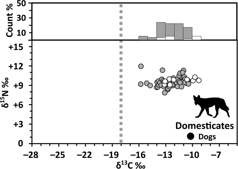
Figure 10. Bivariate plot of bone collagen δ13C and δ15N (lower panel) and δ13C % frequency histogram (upper panel) for Early (white) and later (gray) OIT domestic dogs. Gray dashed line shows cutoff value for diets including foods with C4-derived carbon (for discussion, see Analytical and Interpretive Framework section).
Animal δ15N varies widely but generally follows expected patterns, with carnivores (n = 29, mean = +9.3 ± 1.2‰; Figure 9) on average 4.1‰ higher than herbivores (n = 377, mean = +5.2 ± 2.0‰; Figures 3 and 5–7). Omnivore δ15N (n = 175, mean = +6.7 ± 1.5‰) falls between these trophic levels, and the values suggest that bears (n = 39, mean = +5.5 ± 0.9‰) were primarily herbivorous, whereas raccoons (n = 45, mean = +8.7 ± 1.1‰) were more carnivorous. The large range (13.8‰) of variation observed among δ15N of all herbivore taxa indicates that substantial variation occurred in nitrogen cycling and inputs across the region during the Late Woodland. As observed previously in maize and passenger pigeons from some of these same sites (Guiry et al. Reference Guiry, Orchard, Royle, Cheung and Yang2020), among all species (except for red squirrels and ruffed grouse), there was a significant positive correlation between δ15N and δ13C (see Supplemental Table 7; Spearman's ρ test, p < 0.05), possibly reflecting the impact of Iroquoian horticultural activities on N cycling in gardened areas.
For δ13C, we found no statistically significant differences between any Early and later OIT fauna (compared as ecological groups or individual species; i.e., p always > 0.05; see Supplemental Table 8). When samples from the Princess Point site were removed from respective Early OIT datasets, however, a slight (0.18‰ decrease over time) but significant difference was found between Early and later OIT squirrels (Mann-Whitney U = 2434.5, p = 0.014). Comparisons among individual squirrel species show that this difference is only significant for—and, consequently, driven by—gray squirrels (Mann-Whitney U = 856.0, p = 0.022). For δ15N, we found no statistically significant differences between Early and later OIT specimens for any species or ecological group (regardless of inclusion of Princess Point samples) except for turkeys (Student's t = 3.004, df = 71, p = 0.004), which showed a 0.82‰ increase over time (0.84 when Princess Point samples are removed; Student's t = 2.875, df = 69, p = 0.005).
Discussion
Before considering isotopic evidence for the relative importance of garden resources in animal diets as an indicator for hunting pressure, it is worth exploring other factors that could contribute to patterns in maize consumption. The time frame examined in this study includes periods of climate variability (i.e., the warmer “Medieval Climate Anomaly” followed by the cooler “Little Ice Age”) that could have influenced maize cultivation and hunting. There is, however, ample isotopic (in humans and dogs), archaeobotanical, and other evidence (Katzenberg Reference Katzenberg, John Staller and Benz2006) that maize use was more significant in the latter portion of our study time frame despite climatic cooling. Consequently, we do not consider climatic change further here.
Regardless of local hunting pressure, we expect that some animals will have been hunted farther from settlements, not in close proximity to maize gardens. But because local hunting would have been a more easily accessible source of animals (there is also ethnographic evidence that people did hunt closer to settlements; e.g., Heidenreich Reference Heidenreich1971:206; Tooker Reference Tooker1964:65), patterns observed in our data should be most strongly influenced by animal behavior closer to settlements. Moreover, in addition to providing meat and fur, the hunting of animals in and near maize gardens would be further incentivized as a form of pest removal (Conover Reference Conover2001; Scott Reference Scott2003; ethnographically observed: Heidenreich Reference Heidenreich1971:177–178; Kalm Reference Kalm1964:52; Waugh Reference Waugh1916:36–37). It is also possible that animal behavioral ecology, particularly learned predator avoidance in the context of “landscapes of fear” (Bleicher Reference Bleicher2017), could have played a role in discouraging animals from approaching areas utilized by OIT peoples. Modern studies (e.g., Demeny et al. Reference Demeny, McLoon, Winesett, Fastner, Hammerer and Pauli2019), however, show that maize agriculture is a powerful attractant for all of the animals included in this study, even in contexts where animals risk being hunted. Maize, in fact, is an effective bait used by contemporary hunters across the Northeast (e.g., Kilpatrick et al. Reference Kilpatrick, Labonte and Barclay2010). Moreover, our data show that some animals were able to access maize gardens for substantial periods of time and provide confirmation that animals did not necessarily avoid human areas. For these reasons, we believe that our data do not reflect a scenario in which animals intentionally avoided maize gardens, nor do they reflect one in which garden hunting was not important. Consequently, our results appear to confirm hypothesis 1, which suggests that isotopically meaningful levels of maize consumption (demonstrated across a range of micromammals; see Figures 2 and 3) would have been possible for animals with sufficient access to garden resources.
Concurrently, our results are not supportive of hypothesis 2 (i.e., that evidence from maize consumption in larger animals would decrease between the Early and the later OIT), indicating that the extent to which animals were accessing maize gardens did not change through time. Although a statistically significant shift in δ13C between the Early and the later OIT was observed for a single squirrel species, the shift is small, and, overall, we do not consider this a robust temporal indicator for broad-scale changes in animals’ access to maize. In turn, this suggests that hunting pressure in the general vicinity of OIT sites was high across the Late Woodland, and it implies that hunting (in gardens or farther afield) occurred at a sufficient intensity to largely exclude medium-sized to large animals from spending any significant amount of time in maize fields. To interpret this finding, it is useful to review some of the tremendous environmental and cultural changes that occurred in OIT societies during the Late Woodland.
There is continuity between the earlier, semisedentary communities and the more permanent village communities that develop in the thirteenth and fourteenth centuries in the study area (see Birch Reference Birch2015). The growth rate curve presented by Warrick (Reference Warrick2008:150) shows that the regional population in the North Shore, Georgian Bay of Lake Huron, and Wendake areas grew from about 3,000 to 9,500 people between AD 1000 and 1300, then ballooned to 24,000 people around AD 1330–1420 before leveling off at about 30,000 people after AD 1450 through to contact (Birch Reference Birch2015). Although new excavations of additional village sites since Warrick's (Reference Warrick1990) initial analyses may alter these estimates somewhat (Birch Reference Birch2015), it is clear that demographic growth would have necessitated substantial territorial expansion. By the early fourteenth century, settlement sizes had doubled (Dodd et al. Reference Dodd, Poulton, Lennox, Smith, Warrick, Ellis and Ferris1990) as people aggregated into larger communities, perhaps as an adaptation to the requirements of sedentary life and horticulture. In the mid-fourteenth to early fifteenth century, site sizes become more variable and smaller, possibly reflecting fission of early, larger villages and a more dispersed settlement strategy (Birch Reference Birch2015). Typically, these sites show less defensive infrastructure and an almost complete lack of evidence for conflict-related skeletal trauma on human remains, likely indicating a period of lower conflict (Birch Reference Birch2015). In the mid-fifteenth century (and into the sixteenth century) smaller villages again begin to coalesce, and there is increased evidence for violence (e.g., butchered human remains, heavily fortified villages in defensive positions; Birch Reference Birch2015).
Several factors may contribute to these trends, but a prominent one in the debate about demographic change and conflict is competition for resources. By considering settlement density and the ranging behavior of deer, Gramly (Reference Gramly1977) was the first to propose that the need for deer skin (for clothing) would have outstripped the supply of deer in the local area and, therefore, that deer hunting territory could have been a major source of tension driving increasing conflict. At a large sixteenth-century site, Needs-Howarth and Williamson (Reference Needs-Howarth and Williamson2010) and Birch and Williamson (Reference Birch and Williamson2013:113–120) calculated that a hunting territory with a radius of approximately 20 km around the site would be needed to meet the community's clothing requirements, a region far exceeding the land base (ca. 2 km radius) that would have been under direct cultivation by that community (Birch Reference Birch2015; Birch and Williamson Reference Birch and Williamson2013:95–103). This hunting territory would act as a sink, in which deer populations were depressed and to which deer from source areas would be continually drawn in. Our isotopic data, which show that deer—and most animals—did not have sustained access to maize, are consistent with these arguments, but they also indicate that substantial hunting pressure dates back to the Early OIT in the local area.
Although for economically key taxa, such as deer, evidence that maize use was virtually absent throughout the Late Woodland may not be surprising, the low frequency of maize consumption observed across all taxa suggests that the trends hypothesized for depression of deer populations by Gramly (Reference Gramly1977; cf. Birch and Williamson Reference Birch and Williamson2013:113–120) may be applicable to all animals hunted by humans. Less is known about the importance of other mammals as sources of fur and meat prior to contact. Ethnographic records highlight the importance of fish and large, charismatic species—such as bear (perhaps mirroring the ethnocentricities of the historical writers)—but these sources give us little quantitative or relative information about other species that could also have been important food resources.
Considering the population explosion of the fourteenth century, it is unsurprising that most animals were not accessing maize in the later OIT. However, based on longer-term demographic and settlement trends evidenced in the archaeological record, we expected to see more access to maize among less economically significant taxa. In contrast to the later OIT, with larger, year-round villages, Early OIT communities were smaller and are thought to have been semisedentary (Creese Reference Creese2013; Smith Reference Smith and Dieterman2002; Williamson Reference Williamson, Ellis and Ferris1990). If Early OIT were semisedentary, their horticultural practices may have involved less supervision of maize gardens, which could allow animals more access. The low frequency of maize consumption among Early OIT fauna at these sites suggests that this was not the case, which, if widespread, has two important implications. First, it implies that hunting pressure was sufficiently high for all relevant mammalian taxa that it prevented most animals from substantively accessing maize ecosystems. In turn, it implies that hunting and trapping activities likely occurred year-round in the vicinity of maize fields, and it suggests a degree of permanency in Iroquoian presence in each location (e.g., Creese Reference Creese2013).
Although it appears that small animals were largely excluded from widespread access to maize, subtle isotopic patterns may provide new insights into the relative value of small-mammal furs. For instance, among the squirrel species in our sample (Figure 5), for both Early and later OIT time frames, chipmunks (19.2%, n = 52) and red squirrels (25.9%, n = 27) appear to be consuming maize more frequently than gray squirrels (12.6%, n = 103). Assuming that dietary and environmental preferences of these taxa do not influence their relative use of maize, although not studied directly, these species show strong circumstantial evidence for active maize consumption (see Supplemental Text 5), and this suggests that chipmunks and red squirrels may have been hunted with less intensity than gray squirrels. Perhaps the smaller body size of chipmunks and red squirrels made them less appealing or more difficult targets for trapping (although there is at least some historical evidence of their capture; e.g., Sagard-Theodat et al. Reference Sagard-Theodat, Wrong and Langton1939:223). We would, however, expect the intensity with which these animals were trapped to reflect, among other things, their fur value. Ethnographic observations indicate that squirrel furs were particularly prized for clothing, especially for higher-status items (Sagard-Theodat et al. Reference Sagard-Theodat, Wrong and Langton1939:224; Thwaites Reference Thwaites1896–1901:7:13, 17:165, 243). The effort invested in squirrel trapping is illustrated by multiple references to squirrel-skin garments among Indigenous groups in the Lower Great Lakes and St. Lawrence regions, one even including furs from at least 60 individuals (e.g., Sagard-Theodat et al. Reference Sagard-Theodat, Wrong and Langton1939:224; Thwaites Reference Thwaites1896–1901:7:13, 17:165, 243). Among squirrel pelts, color may have been significant, with a preference for black color morphs of the gray squirrel (Thwaites Reference Thwaites1896–1901:17:243). Curiously, no similar references to the furs of chipmunks and red squirrels appear in these historical accounts, despite their distinctive dorsally striped (white, black/brown, orange) and red coat, respectively (e.g., Sagard-Theodat et al. Reference Sagard-Theodat, Wrong and Langton1939:222–223). In this context, the isotopic difference between types of squirrels could reflect a long-standing pattern in fur preferences.
Our findings are also useful for reconsidering previous hypotheses about the isotopic compositions of Late Woodland human and dog bone collagen, both of which suggest significant amounts of maize consumption across the region (Figure 10; Katzenberg Reference Katzenberg1989; Morris Reference Morris2015). The lack of maize consumption among most mammals means that the maize-derived carbon contributing to higher human and dog bone collagen δ13C is coming directly from eating maize and/or possibly caecotrophy in the case of dogs (Guiry Reference Guiry2012; both consistent with ethnographical evidence suggesting that dogs were free to scavenge refuse and leftovers; Heidenreich Reference Heidenreich1971:105) rather than consumption of animals that had consumed maize. The exception to this is micromammals. Mice and meadow voles were collected for human consumption (e.g., Sagard-Theodat et al. Reference Sagard-Theodat, Wrong and Langton1939:227; Waugh Reference Waugh1916:135), but little is known about their relative dietary importance. Ethnographical evidence suggests that these were collected using traps (e.g., Sagard-Theodat et al. Reference Sagard-Theodat, Wrong and Langton1939:227), but the value of carnivorous domesticates for pest control was also recognized (Sagard-Theodat et al. Reference Sagard-Theodat, Wrong and Langton1939:270; in this case, a cat requested as a gift from the French). Given their small size, we suspect that micromammals were of lesser overall importance for human diets (but see Stahl Reference Stahl1982). For dogs, however, higher bone collagen δ13C would be consistent with substantial consumption of mice and voles (Figure 10). Given that evidence for higher bone collagen δ13C in dogs is widespread in North America (e.g., Allitt et al. Reference Allitt, Michael Stewart and Messner2008; Burleigh and Brothwell Reference Burleigh and Brothwell1978; Guiry Reference Guiry2013; Tankersley and Koster Reference Tankersley and Koster2009; White et al. Reference White, Pohl, Schwarcz and Longstaffe2001), this finding may also be of interest for interpretations of dog diets at sites in other regions.
The roles that dogs have played in Late Woodland societies is a topic of growing interest, and our small-mammal data also provide a novel perspective for evaluating theories about the uses of dogs (see Supplemental Text 6). Campbell and Campbell (Reference Campbell and Campbell1989) hypothesized that an important role of dogs in Iroquoian society was in controlling groundhog populations and that, because groundhogs were a major source of food for dogs, groundhog population sizes might be an important predictor of dog population sizes. Indeed, several ethnographic sources indicate that groundhogs were an important garden pest (e.g., Waugh Reference Waugh1916:37). Interestingly, however, our data suggest that although groundhogs may have lived in maize gardens, they were not depredating maize. In fact, they have some of the lowest δ13C values of any taxa observed across the entire Late Woodland forest ecosystem (Table 3; Figure 6). Moreover, given the very high δ13C values for dogs (Figure 10; e.g., Katzenberg Reference Katzenberg1989; Morris Reference Morris2015), it seems unlikely that they consumed groundhogs in any significant numbers. In turn, assuming that dogs would have taken advantage, at least occasionally, of the small animals they hunted (particularly the less valuable pest taxa) as a source of food, it seems unlikely that groundhog population control was an important role for dogs.
Summary and Conclusion
In this article, we have characterized the isotopic ecology of a later-Holocene agroforest ecosystem to (1) provide a novel perspective on the extent to which animals were accessing anthropogenic maize gardens, with the goal of (2) exploring patterns in resource depression resulting from local animal hunting. Our results suggest that, although isotopic evidence for animal use of maize resources does provide a meaningful indication for relative differences in access to maize between species (consistent with hypothesis 1), corresponding interpretations of hunting pressure should be limited only to the local area (inconsistent with hypothesis 2). Our study suggests that hunting pressure broadly limited animals’ access to maize resources in both the Early OIT and the later OIT and, therefore, that hunting pressure in the vicinity of settlements was likely high throughout the Late Woodland. Interestingly, these results suggest a relatively permanent presence of humans in the vicinity of Early OIT gardens, such that animals other than micromammals were largely prevented from accessing maize. In this way, our results provide a novel perspective on land management during the early years of the adoption of horticulture in the region.
With respect to using isotopic analyses for exploring resource depression, our findings are mixed. The lack of a relationship between animal access to maize and major indices for cultural changes across the Late Woodland—such as increasing sedentism and population size—suggests that the isotopic approach employed here, although effective, should be limited to research questions focused on localized resource depression and source–sink dynamics. Considering the growing interest in isotopic approaches to garden hunting across many regions of the Americas and Asia (e.g., Morris Reference Morris2015), this approach may provide a useful tool for complementing traditional zooarchaeological methods for studying resource depression in spatiotemporal contexts where C4 plants—such as millet, maize, and sugarcane—were being domesticated or introduced. It is, however, important to remain cognizant of potential sources of naturally occurring C4 plants. In contexts where a substantial fraction of local flora may be composed of C4 plants, it is critical to include meaningful control samples of animals (ideally from the same species) that predate the introduction of the C4 cultigen(s).
From a methodological perspective, our results showcase how including a larger range of archaeologically available species in isotopic analyses of terrestrial ecosystems can support a wider and more nuanced set of interpretations. The large number of taxa included here has enabled us to contrast results between different “ecological perspectives” brought by unique aspects of the ecology of each taxon to provide a more robust framework for interpreting animal use of maize gardens. This is particularly true for small mammals, which are often overlooked in archaeological isotopic research. Our results show not only that a substantial fraction of small-mammal remains are likely contemporaneous with site occupation, but also that they can provide key “ecological anchor points” for interpreting trends in animal access to anthropogenic resources, such as maize. In turn, results from small mammals enabled us to explore a wide range of cultural phenomena, including hunting pressure on larger animals, methods of pest control, and the relative value placed on small-mammal furs.
Acknowledgments
Eric Guiry was supported by a SSHRC Banting Fellowship. Analyses supported by the Department of Anthropology at the University of British Columbia and a SSHRC Insight Development Grant. We thank both the Department of Anthropology at the University of Toronto Mississauga and Archaeological Services Inc. (ASI) for permission to collect samples as well as Stéphane Noël for assistance with abstract translation. We appreciate the privilege of studying the archaeology of First Nations peoples across southern Ontario and acknowledge that the faunal remains analyzed here are from archaeological sites located in the ancestral and traditional territories of multiple First Nations, including the Wendat, Tionontati, Attawandaron, Haudenosaunee, and Mississauga. Suzanne Needs-Howarth is also affiliated with Trent University Archaeological Research Centre, 1600 West Bank Drive, Peterborough, ON K9L 0G2, Canada. The authors declare no conflicts of interest.
Authorship Statement
Conceptualization (EG/TJO), Methodology (EG), Investigation (EG/TJO/SNH), Formal Analysis (EG), Data Curation (EG), Visualization (EG), Project Administration (EG), Resources (EG/TJO/PS), Funding Acquisition (EG), Writing—Original Draft (EG/TJO), Writing—Review and Editing (EG/TJO/SNH/PS).
Data Availability Statement
All data presented in this manuscript are available in the Supplemental Materials.
Supplemental Materials
For supplemental material accompanying this article, visit https://doi.org/10.1017/aaq.2020.86.
Supplemental Text 1. Isotopic studies of maize use in modern ecosystems.
Supplemental Text 2. Additional archaeological context and sample description.
Supplemental Text 3. Collagen extraction for radiocarbon dating.
Supplemental Text 4. Data calibration.
Supplemental Text 5. Studies of Sciuridae maize use.
Supplemental Text 6. Studies on the roles of dogs.
Supplemental Table 1. List of archaeological sites and context information.
Supplemental Table 2. Isotopic compositions for standards used in this study.
Supplemental Table 3. Standard deviations for calibration standards.
Supplemental Table 4. Means and standard deviations for calibration standards.
Supplemental Table 5. Standard deviations for sample replicated.
Supplemental Table 6. Stable isotope and elemental compositions of samples.
Supplemental Table 7. Statistical comparisons of group means.
Supplemental Table 8. Results of Spearman's rho testing for intragroup correlations.


