Archaeologists are keen to understand the ways in which past mobile foragers organized and scheduled their activities on the landscape. A key to this goal is to reconstruct how, when, and where people moved to carry out activities and procure resources (Kuhn et al. Reference Kuhn, Raichlen and Clark2016). Because movement itself usually leaves no lasting material trace, to infer past mobility, archaeologists rely heavily on physical remains that are indicative of transport, such as raw material sourcing (Féblot-Augustins Reference Féblot-Augustins1993, Reference Féblot-Augustins1999; Fernandes et al. Reference Fernandes, Raynal and Moncel2008; Turq et al. Reference Turq, Faivre, Gravina and Bourguignon2017). Yet, interpreting human movement from raw material sourcing is not a straightforward task. Although sourcing can demonstrate that an object has been transported from Point A to Point B, the data say little about how people actually moved (Close Reference Close2000). At the heart of this issue is equifinality, where similar archaeological patterns can emerge via dissimilar movement processes. For instance, the same transport from Point A to B could have occurred either as a single, long, linear journey or as a winding path, consisting of many turns connected by shorter segments—or “steps” (Brantingham Reference Brantingham2006). Knowing the distance between A and B does not help one discern between these two possibilities (or others). What is more, because stone is durable, previously discarded lithics visible on the surface can be picked up, reused, and moved subsequent to their initial discard (Dibble et al. Reference Dibble, Holdaway, Lin, Braun, Douglass, Iovita, McPherron, Olszewski and Sandgathe2017; Holdaway and Douglass Reference Holdaway and Douglass2012). Finally, stone artifacts accumulate differentially on the landscape due to the organization of the lithic technology, procurement costs and return rates, place use duration, group size, and the frequency of revisits to previously occupied localities (Andrefsky Reference Andrefsky2009; Binford Reference Binford1980; Kuhn Reference Kuhn1995; Schiffer Reference Schiffer1976; Shott Reference Shott1989; Surovell Reference Surovell2012). As such, the details concerning where and how far raw materials are transported are emergent properties of the archaeological record that reflect—and in some cases, distort—the ways foragers managed stone resources over time (Režek et al. Reference Režek, Dibble, McPherron, Braun and Lin2018, Reference Režek, Holdaway, Olszewski, Lin, Douglass, McPherron, Iovita, Braun and Sandgathe2020).
To begin to tackle the complexity of archaeological landscape formation, researchers have increasingly employed an agent-based modeling approach to investigate movement scenarios that generate simulated outcomes that are comparable (in at least one way) to empirical patterns (Barton and Riel-Salvatore Reference Barton and Riel-Salvatore2014; Brantingham Reference Brantingham2003, Reference Brantingham2006; Davies Reference Davies2016; Davies et al. Reference Davies, Holdaway and Fanning2018; Haas and Kuhn Reference Haas and Kuhn2019; Oestmo et al. Reference Oestmo, Janssen and Cawthra2020; Pop Reference Pop2016; Reeves Reference Reeves2019). The neutral procurement model developed by Brantingham (Reference Brantingham2003, Reference Brantingham2006) has received considerable attention. Brantingham studied the raw material distribution patterns that were generated under nondirected mobility and raw material acquisition. His models showed that the distance-decay distribution of raw material abundance commonly observed among archaeological assemblages (Féblot-Augustins Reference Féblot-Augustins1993, Reference Féblot-Augustins1997, Reference Féblot-Augustins1999, Reference Féblot-Augustins and Pearsall2008; Geneste Reference Geneste1985) can emerge despite “neutral” assumptions regarding movement and raw material preference (Brantingham Reference Brantingham2003). Moreover, by using a Lévy walk function, his model further demonstrated that differences in how far raw material can travel can be explained by changes in the frequency of long “step lengths,” without invoking a wholesale change in hominin mobility (Brantingham Reference Brantingham2006).
Brantingham's neutral model has been criticized for its simplicity and lack of realism (Duke and Steele Reference Duke and Steele2010). But the value of modeling is arguably not in its capacity to replicate real-world phenomena under “realistic” settings. Instead, the approach offers an experimental tool to explore nonlinear dynamics in archaeological formation as a means to generate new hypotheses that hopefully can be tested against archaeological—rather than simulated—data (Premo Reference Premo2006, Reference Premo, Costopoulos and Lake2010). Instead of aiming for “realism,” a model's utility depends to a large extent on how well its underlying assumptions represent—albeit in an abstract and simplified form—the essence of the real-world phenomenon it seeks to investigate (Cegielski and Rogers Reference Cegielski and Daniel Rogers2016). Different researchers may very well have different ideas regarding what the essence of the system under investigation is. This is to be expected and encouraged. Building middle-range theory in this way allows one to learn more about which factors have an important causal relationship with archaeological signals we can detect, and—just as importantly—which factors do not. To this end, subsequent studies have expanded on Brantingham's neutral model to investigate how other variables influence archaeological landscape-scale patterns. For instance, later studies show that variation in the density and clustering of raw material sources can significantly impact archaeological landscapes (Oestmo et al. Reference Oestmo, Janssen, Marean, Barceló and Castillo2016; Pop Reference Pop2016), a finding that highlights the importance of understanding the geology specific to a region before applying the neutral procurement model to infer past behavior (Duke and Steele Reference Duke and Steele2010; Oestmo et al. Reference Oestmo, Janssen and Cawthra2020).
In our opinion, another parameter in Brantingham's neutral model that requires further scrutiny is tool discard probability. In keeping with the neutral model condition, Brantingham (Reference Brantingham2003, Reference Brantingham2006) held tool discard probability constant at 1. But as Shott (comment in Brantingham Reference Brantingham2006) remarked, the fact that foragers discard different tool types at different rates may have an important influence on lithic assemblage variability (Kuhn Reference Kuhn1994; Schiffer Reference Schiffer1987; Surovell Reference Surovell2012). More specific to the question at hand, it is important to clarify how tool discard probability affects raw material transport under a range of mobility strategies before proposing that perceived shifts in archaeological raw material distributions were caused mainly by changes in hominin mobility. To jump right into interpreting what the archaeological pattern “means” in terms of mobility alone, without fully understanding the causal relationship between process (i.e., past behavior) and pattern (i.e., distance to source data), is to put the cart before the horse.
To continue to build the middle-range theory required to infer an unobservable cause (a purported change in hominin behavior[s]) from an observed effect (a perceived shift in an archaeological signal), this study uses a modified version of Brantingham's (Reference Brantingham2006) Lévy walk model to investigate the effect of tool discard probability on distance to source data. The results show that decreasing discard probability affects distance to source distributions in a way that is similar to increasing the likelihood of embarking on longer “steps.” The take-home lesson of our simulation experiment is that quantitative changes to either forager mobility or discard behavior can yield similar patterns in distance to source data. Faced with equifinality, additional lines of evidence are required to disentangle the respective effects of discard probability and mobility.
Brantingham's Neutral Model of Stone Procurement
Brantingham's spatially explicit neutral model assumes that the environment is uniform in terms of food sources, that there is no pressure of raw material supply, and that each forager moves in a nondirected way on the model space. Each forager carries a mobile stone toolkit, marked by a maximum size of 100 tools, from which the forager discards one tool during each simulated time step until the toolkit is depleted. Brantingham studied two iterations of this basic model. The first model (Brantingham Reference Brantingham2003) involved a single forager engaging in a Brownian-like random walk through a two-dimensional world composed of 500 × 500 cells. In each simulation, the world is populated with raw material sources distributed randomly in space. Each source represents a unique type of stone. During each time step of the simulation, the forager moves to one of its nearest eight neighboring cells or stays in its current cell—each of the nine options occurs with equal probability. When a raw material source is encountered, the forager collects enough raw material to “top off” its toolkit to the maximum capacity (which, in this case, is 100 units). During each time step, if the toolkit is not empty, the forager discards one tool from the toolkit. The raw material type assigned to the discarded artifact is a function of the relative frequencies of the raw material types present in the forager's toolkit. This neutral assumption represents a process of blindly grabbing (or randomly sampling without replacement) a stone tool from the toolkit irrespective of which raw material type might be “preferred” due to its toolmaking properties or availability on the landscape.
This iteration of the neutral model is used to study how far raw material travels from its source under the assumptions that forager movement is nondirected (i.e., random) and that no raw material type is preferred over others. One of the main findings is that the right-skewed frequency distribution of the simulated distance to source data superficially resembles the distance-decay pattern observed in Middle Paleolithic assemblages in Europe. On the basis of this proof of concept, Brantingham (Reference Brantingham2003) suggests that the neutral scenario, whereby stone procurement is nonselective and embedded within other foraging activities that are not directed toward the sources of raw material, may be sufficient to explain the distance to source distribution exhibited by European Paleolithic stone tool assemblages. The fact that the model is so simple makes the finding all the more powerful and thought provoking.
Brantingham (Reference Brantingham2006) incorporated the Lévy walk in the second iteration of the neutral model. In this case, the forager agent moves in a randomly chosen direction, but the distance of the “step” is determined not by the move into a neighboring cell but by a stochastic process known as the Lévy walk. The Lévy walk function follows a power-law distribution with a heavy tail, meaning that the likelihood of a step length of x diminishes quickly with increasing x. The mean and shape of the distribution can be altered by changing the μ parameter in the probability function. When μ is relatively high (≥3), the mean of the step length distribution is low, resulting in a Brownian-like random walk where virtually all moves occur over short distances (this is similar to the first iteration of the model). However, decreasing μ increases the likelihood of longer step lengths. Despite its simplicity—or perhaps because of it—the Lévy walk has been shown to capture the general movement patterns of many organisms (Humphries et al. Reference Humphries, Weimerskirch, Queiroz, Southall and Sims2012; Sims et al. Reference Sims, Humphries, Bradford and Bruce2012; Viswanathan et al. Reference Viswanathan, Afanasyev, Buldyrev, Murphy, Prince and Stanley1996), including the foraging patterns of humans (Brown et al. Reference Brown, Liebovitch and Glendon2007; Raichlen et al. Reference Raichlen, Wood, Gordon, Mabulla, Marlowe and Pontzer2014). Importantly, for the present application, the Lévy walk approach does not assume a priori the forms of mobility strategies practiced by past foragers. Brantingham (Reference Brantingham2006:437) contends that whether or not the steps between endpoints are to be interpreted as logistical foraging trips or residential moves depends on the spatial and temporal scales of the model. Brantingham (Reference Brantingham2006:444) interprets the endpoints of each Lévy “step” as representing residential bases.
Unlike the first iteration of the neutral model, in which the “world” is seeded with many unique stone sources, Brantingham's Lévy walk model contains just a single raw material source at the center of the world. During each simulation, a single forager engages in a Lévy walk. Each “step” of the Lévy walk involves first resetting the forager's bearing to a value chosen randomly from a uniform distribution bound by 0 and 360 and then determining the length of the “step” it will travel in that heading by sampling a value from the Lévy walk function parameterized by a given μ. Once the length and heading of the step are set, the forager embarks on this linear segment. Each time step of the simulation allows the forager to move one spatial unit along its path. At each incremental step along the path, the forager can detect the presence of the raw material source within its field of vision defined by a radius of 0.5. Whenever the raw material source is encountered, the forager “tops off” its toolkit to the maximum size of 100 units. As in the first iteration of the model, stone tool use is assumed to occur continuously, and as a result, one unit of stone is discarded during each time step of the simulation for as long as the toolkit contains raw material. The simulation records the distance between each cell that contains at least one discarded tool and the raw material source in the center of the spatial world.
This Lévy-walk version of the model also generated distance to source distributions marked by the familiar distance-decay profile (see Figures 11–13 in Brantingham Reference Brantingham2006). Brantingham shows how μ affects distance to source. For high values of μ (μ ≥ 3), the vast majority of tools are discarded in cells that are relatively close to the raw material source. As μ decreases and longer step lengths become more common, the mean, mode, and skewness of the distance to source distribution increase. Here again, the simulated data show some similarity, at least impressionistically, to the Paleolithic archaeological record of Europe (Féblot-Augustins Reference Féblot-Augustins1993, Reference Féblot-Augustins1997, Reference Féblot-Augustins1999). It is commonly noted that Middle Paleolithic assemblages seem to be dominated by tools made on raw material procured from sources located within 10 km of the sites, with very few tools made on so-called nonlocal raw material (Féblot-Augustins Reference Féblot-Augustins1993, Reference Féblot-Augustins1997, Reference Féblot-Augustins1999, Reference Féblot-Augustins and Pearsall2008). By contrast, Upper Paleolithic assemblages seem to be marked by a greater proportion (though still a minority) of tools made on raw materials from sources located tens to hundreds of kilometers away from the site in which they were ultimately discarded (Féblot-Augustins Reference Féblot-Augustins1997, Reference Féblot-Augustins1999, Reference Féblot-Augustins and Pearsall2008, Reference Féblot-Augustins, Adams and Blades2009). The results of Brantingham's Lévy walk model raise the possibility that the perceived shift from a focus on closely adjacent raw materials to apparently incorporating at least some raw materials from farther afield may reflect a greater tendency for Upper Paleolithic hominins to undertake longer distance moves or “steps” (i.e., lower μ), holding all else constant. When combined with the assumption (not necessarily espoused by the authors of this article) that Middle Paleolithic tools were made exclusively by Neanderthals and that Upper Paleolithic tools were made exclusively by modern humans, this lends some support to the notion that Neanderthals were less mobile than modern humans perhaps due to population-level differences in biomechanical energetics, social networks, or land-use strategies (Barton et al. Reference Barton, Riel-Salvatore, Anderies and Popescu2011; Féblot-Augustins Reference Féblot-Augustins and Pearsall2008; Riel-Salvatore and Barton Reference Riel-Salvatore and Michael Barton2004; Steudel-Numbers and Tilkens Reference Steudel-Numbers and Tilkens2004; Verpoorte Reference Verpoorte2006; Weaver and Steudel-Numbers Reference Weaver and Steudel-Numbers2005). Although it may go without saying, it is worth noting here that Brantingham's model results do not rule out other possible explanations for what is perceived to be a shift toward nonlocal raw material sources.
Brantingham (Reference Brantingham2006) focuses on how changing hominin mobility strategies might affect distance to source distributions in archaeological landscapes. He (correctly) investigates this causal relationship by varying μ while holding constant all other parameters, including discard probability. To date, relatively little attention has been paid to how changes in tool discard might affect distance to source distributions in archaeological landscapes. In simple terms, discard is the process by which material objects are disposed from the systemic tool inventory onto the landscape (Foley Reference Foley1981; Schiffer Reference Schiffer1976). To isolate the effect of μ, Brantingham (Reference Brantingham2003, Reference Brantingham2006) controlled for variation in the discard process by employing a constant discard probability of 1. Shott (comment in Brantingham Reference Brantingham2006) points out that artifact discard is not constant but rather is governed by a suite of factors such as tool function, design and use life, raw material availability/accessibility, and spatial differences in activities (Binford Reference Binford1979, Reference Binford1980; Schiffer Reference Schiffer1987; Shott and Sillitoe Reference Shott and Sillitoe2005). In the case of curation, for example, expedient flake tools generally have a shorter use life and therefore would be discarded with a higher probability per unit time than items such as hafted adzes and axes, which are maintained and used over longer periods before they are discarded (Keeley Reference Keeley1982; Odell Reference Odell and Odell1996). In addition, the likelihood that a tool is discarded may also depend on the availability of the raw material required to replace it (Andrefsky Reference Andrefsky1994; Garvey Reference Garvey, Goodale and Andrefsky2015). Tools that can be easily replaced because the materials needed to do so are close at hand may have a higher discard probability for that reason alone (i.e., easy come, easy go). On the other hand, in the absence of readily available raw material, foragers may be forced to curate tools more heavily, thereby decreasing discard probability, regardless of their mobility strategy.
The point to make here is that there is likely considerable variation in the discard behavior of foragers, some of which functioned separately from mobility (Lin Reference Lin2018). And it stands to reason that, just as in the case of mobility (see above), changes to the discard probability are likely to impact the way in which stone tools are distributed on simulated archaeological landscapes. After all, holding all else constant, the total distance a random walker travels before depleting that walker's toolkit increases as discard probability decreases (see the effect of λ on total time steps per simulation run in Supplemental Table 1). Consequently, a lower discard probability should allow artifacts to be deposited at a greater distance from their source on average even when there is no change in μ. These predictions suggest that, in addition to changes in forager mobility, changes in discard probability (i.e., technological curation) could have important effects on the spatial distribution of stone tools. Here, we build on Brantingham's Lévy walk model (Reference Brantingham2006) to investigate how discard probability affects distance to source of stone tools under different values of μ.
Modifying the Neutral Model to Investigate the Effect of Discard Probability
We employ a modified version of Brantingham's agent-based Lévy walk model. The fully documented NetLogo (Wilensky Reference Wilensky1999) and R (R Core Team 2021) source code files used in this study are archived on the open-access repository of Zenodo (DOI:10.5281/zenodo.5035823).
The model space is a two-dimensional grid composed of 1,000 × 1,000 square cells. As in Brantingham (Reference Brantingham2006), a single raw material source is located at the center of the model space. Unlike Brantingham's model, each of our simulation runs starts with 50 forager agents on the raw material source. Because foragers do not interact with each other directly or indirectly (i.e., previous actions, like discarding a tool, do not affect the shared environment in ways that influence subsequent actions), the 50 foragers in each simulation represent 50 unique and independent instances of a forager departing from a raw material source with a “full” stone toolkit containing 100 items. In our model, foragers do not “top off” their toolkits if they happen upon the raw material source during the simulation. Each simulation run ends when all foragers have exhausted their toolkits. As a result, each simulation run produces an archaeological landscape that contains exactly 5,000 artifacts.
Each forager agent executes a Lévy walk during the course of the simulation. When a destination has been reached (or at the start of the simulation), a new “step” must be charted by setting a forager's bearing, β, to a value drawn from a uniform distribution bound by 0 and 360, and acquiring the new step's length, l, from the Lévy walk function:

where μ is the critical Lévy walk parameter. Following Brantingham (Reference Brantingham2006), we investigate three values of μ: 1.2, 2.0, and 3.5. Because there is no upper limit to the values the Lévy walk function can generate, it is possible for l to exceed the boundary of the 1,000 × 1,000 cells model world. For this reason, foragers only accept step lengths that allow them to travel to destinations that exist within the space available. Because of working with a finite-sized two-dimensional world, the resulting distribution of l does not reflect a true Lévy walk distribution but rather one in which the tail is truncated by the boundary of the model space. Although the effect of this limitation is larger when μ is low, overall, it does not negatively affect our ability to assess the general effect of discard probability on distance to source.
Once β and l are determined, the forager agent travels the linear path until it reaches its destination. This travel occurs incrementally—one spatial unit traveled per simulated time step—until the forager has traveled the full distance l. Stone tool discard can occur all along the forager's path, not just at its endpoints. During each time step, the forager discards one stone tool from its mobile toolkit with discard probability, λ. Our experimental design investigates three values of λ: 0.1, 0.5, and 0.9. Again, note that our model does not include the “retooling” process described in Brantingham (Reference Brantingham2006). Although it is undeniably an important aspect of lithic technological organization, retooling is unnecessary to our current research aim. More pragmatically, allowing forager agents to refill their toolkits would not alter the results of this model.
Figure 1 summarizes the overall model workflow. We collect data from 50 simulation trials for each combination of the experimental values of the parameters μ and λ. Each simulation ends when the foragers have exhausted their toolkits of all 100 artifacts. Consequently, our experimental design controls for raw material used, the number of tools created, and the distance traveled per time step by each forager across different values of μ and λ. It also controls for the total distance traveled per forager across different values of μ (foragers travel farther over the course of the simulation when λ is lower). At the end of each simulation trial, we record the number of cells that contain at least one discarded tool, hereafter referred to as “discard sites.” In addition, we record the distance between each discard site and the raw material source (from which we can extract the maximum distance to source per simulation run), and the number of tools at each discard site. All analyses were done using the R statistical software (R Core Team 2021). Supplemental Table 1 summarizes mean step length and total time steps per simulation run.
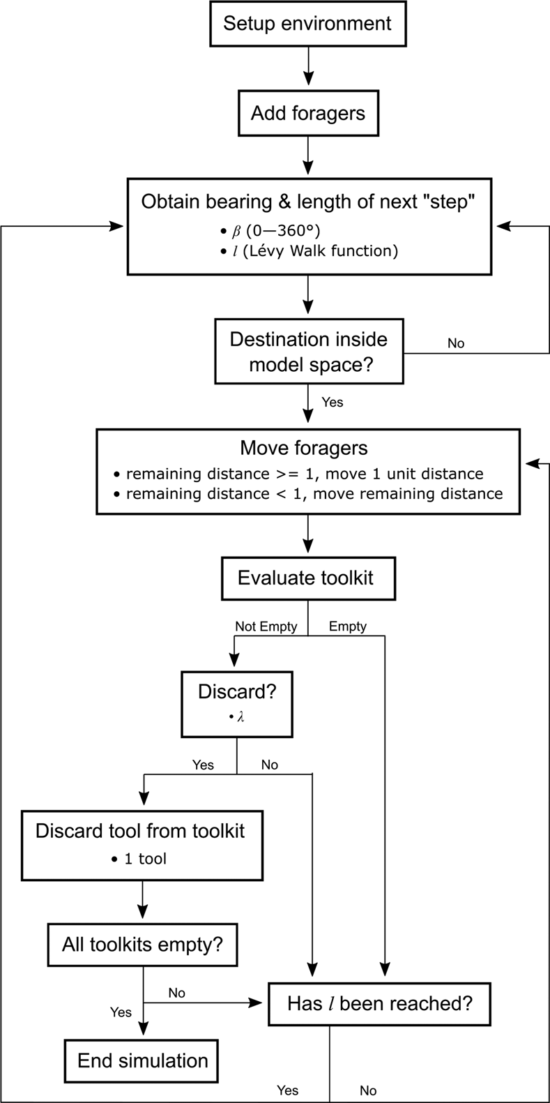
Figure 1. Model workflow.
Results
Distance to Source
Figure 2 provides histograms of the relative frequency of discard sites binned by distance to source for the nine experimental combinations of the Lévy walk parameter (μ) and discard probability (λ) values investigated here. Controlling for λ, the average distance to source increases as μ decreases toward 1. This finding matches Brantingham's (Reference Brantingham2006) previous observation: holding all else constant, decreasing μ increases distance to source. But our results also show that decreasing discard probability (λ) has a similar effect on distance to source. On average, tools are discarded closer to the source when λ is higher (e.g., 0.9) than when λ is lower (e.g., 0.1). In other words, decreasing λ increases the mean, mode, and maximum of the distance to source distribution. This finding is consistent with our earlier prediction that, holding μ constant, higher discard probabilities ought to yield shorter distances to source. Why is this? When λ is high, foragers exhaust their toolkits in fewer time steps, regardless of μ (Supplemental Table 1). With fewer time steps available for movement due to a higher λ, foragers are unable to travel as far before discarding the last of their tools. Although the mechanisms are different, the effect of increasing λ is similar to the effect of increasing μ. And because μ and λ each has a similar effect on distance to source, decreasing both at the same time compounds the negative effects. When μ and λ are low, not only are foragers more likely to embark on longer “steps,” but they also travel farther along their random walks before discarding their last tool (see lower left panel of Figure 2).
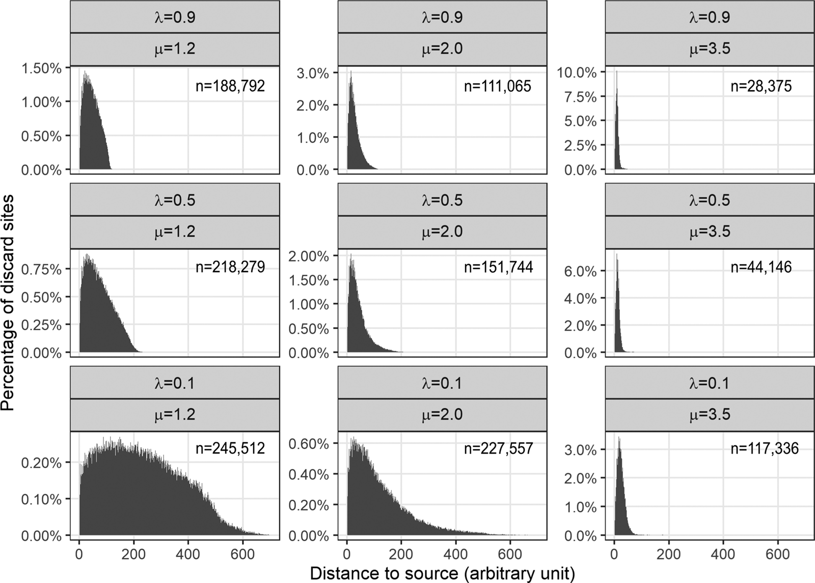
Figure 2. Relative frequency of discard sites by distance to source for nine combinations of μ and λ. The total number of discard sites recorded over 50 simulation runs for each combination of experimental parameter values is provided in the upper-right corner of each panel. Bin width is 1 spatial unit. Distance to source cannot exceed 707.11. The scale of the y-axis varies among panels.
Maximum Distance to Source
Figure 3 plots maximum distance to source by μ and λ. Unsurprisingly, μ and λ each has a negative effect on the maximum distance to source—increasing either λ or μ causes the maximum distance to source to decrease. It is worth noting that the magnitude of the negative effect of μ on maximum distance to source decreases as λ increases. Likewise, the magnitude of the negative effect of λ on maximum distance to source decreases as μ increases. This relationship holds even though our use of a 1,000 × 1,000 cell model space sets an arbitrary “ceiling” of 707.11 on maximum distance to source. If the model space were larger, the effect of λ on maximum distance to source for the case of μ = 1.2 would be even greater than what we observe here.
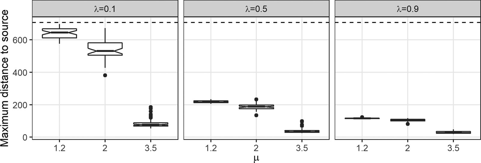
Figure 3. The effect of μ on maximum distance to source for three values of λ. Each boxplot represents 50 data points. The spatial extent of the model world imposes a “ceiling” of 707.11 on maximum distance to source (dashed horizontal line).
Number of Discard Sites
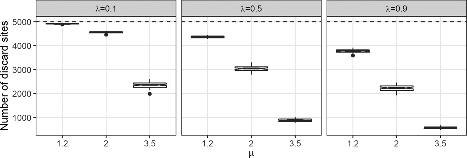
Figure 4 plots number of discard sites by μ and λ. As was the case for maximum distance to source, μ and λ each has a clear negative effect on the number of discard sites. In essence, the number of discard sites per simulation increases when foragers undertake a greater number of longer distance steps (low μ) or when they discard tools less frequently (low λ). A cell can be visited multiple times, but as long as it contains at least one artifact, it counts as just one more discard site, regardless of how many tools it collects over repeated visits. When μ is high, the tendency to travel shorter step lengths means foragers commonly revisit the same cells over and over, depositing most of their toolkits’ contents in a relatively small proportion of the world's 1,000,000 cells. When μ is low, thereby increasing the likelihood of longer step lengths, foragers do not revisit cells as frequently. As a result, tools are distributed more evenly over a larger proportion of the world's cells. Holding μ constant, when λ is high, foragers exhaust their toolkits in fewer time steps, limiting the number of cells they can potentially visit before the simulation ends. As λ decreases, foragers experience longer random walks simply because it takes a greater number of time steps for their toolkits to run dry. As a consequence of traveling a longer random walk, foragers deposit their tools in a greater number of cells when λ is low—especially when μ is also low. Again, mobility and discard probability are two different mechanisms that have similar effects on the number of discard sites in our model. It is important to point out that two of our model assumptions—that all 50 foragers start with 100 tools in their toolkits and that the simulation ends when all toolkits are empty—arbitrarily “cap” the number of discard sites at 5,000. If one increases the number of foragers or the toolkit size and reruns the simulations, the effect of λ on the number of discard sites for μ = 1.2 will be even greater than what we observe here.

Figure 4. The effect of μ on the number of discard sites for three values of λ. Each boxplot represents 50 data points. Note that our model assumptions and parameter values impose a “ceiling” of 5,000 discard sites (dashed horizontal line).
Tools per Discard Site
Figure 5 plots the average number of tools per discard site by distance to source for the nine experimental combinations of μ and λ. Each panel presents data collected from 50 simulations. The leftmost bar in each panel provides the mean number of tools found in all discard sites that are one spatial unit away from the raw material source. The second bar provides the mean number of tools found in all discard sites located between one and two spatial units from the raw material source, and so on. When μ is high, tools are highly concentrated in the relatively few cells closest to the raw material source. This is explained by the fact that foragers frequently revisit cells close to their point of origin as they move about in a Brownian-like fashion. As μ decreases toward 1, increasing the likelihood of longer step lengths, tools are discarded more evenly over a greater number of cells, many of which are located farther from the source. A similar relationship holds for λ. When discard probability is high and foragers deplete their toolkits in fewer time steps, tools are concentrated in cells closer to the source. But as discard probability decreases and foragers travel longer random walks before exhausting their toolkits, tools are distributed over a greater number of cells, including some located at a greater distance from the source.

Figure 5. Average number of tools per discard site as a function of discard sites’ distance to source by μ and λ. Every simulated archaeological landscape contains exactly 5,000 artifacts. Bin width is 1 spatial unit. The x-axis is truncated at 100 merely to aid presentation.
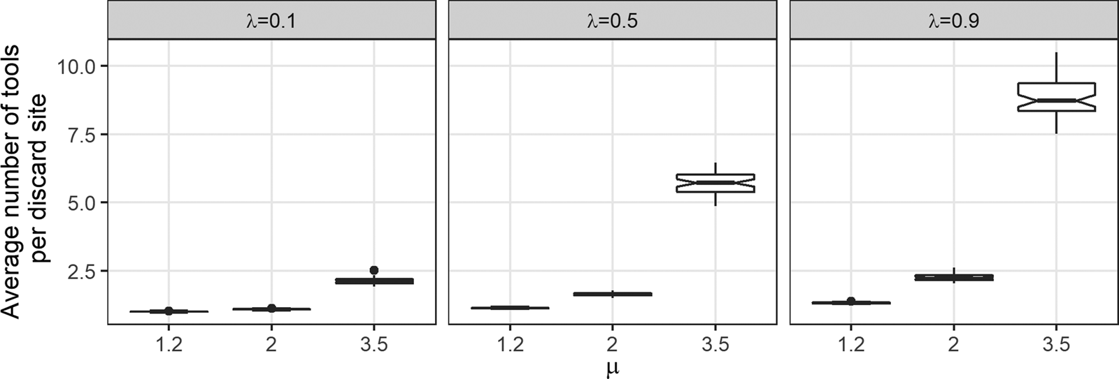
Figure 6 plots the average number of tools per discard site per simulation, this time irrespective of each discard site's distance to source. Because our experimental design controls for the total number of artifacts in each simulated archaeological landscape (5,000 artifacts are deposited per simulation run), any process that reduces the number of discard sites must increase the average number of tools per discard site per simulation. This explains why the relationship between μ and λ and the average number of tools per discard site per simulation (Figure 6) is the inverse of the relationship we observed between μ and λ and the number of discard sites per simulation (Figure 4). Here, both μ and λ have a positive effect on the average number of tools per discard site. The magnitude of the effect of μ increases as λ increases. Likewise, the magnitude of the effect of λ increases as μ increases. It is important to note that because the average number of tools per discard site is a function of the number of discard sites, these do not represent independent lines of evidence given our model design.

Figure 6. The effect of μ on the average number of tools per discard site for three values of λ. Each boxplot represents 50 data points.
Discussion
The results of Brantingham's (Reference Brantingham2006) Lévy walk model suggest that subtle shifts in distance to source during the Paleolithic may have been caused by a quantitative shift in hominin mobility and land use. More specifically, he speculates that an archaeological signal that suggests increased use of nonlocal raw materials might serve as evidence of a shift toward a mobility strategy that required greater planning to accommodate lengthier trips between residential bases. Although there may be some truth to that, the take-home lesson of the current study is that a similar empirical signal can also be explained by a change in tool discard behavior—that is to say, while holding μ constant, decreasing the discard probability also increases the mean and maximum distance to source. Although this outcome is not surprising on its own, it clearly highlights the difficulty of separating the effects of mobility from those of discard when interpreting empirical distance to source data. Indeed, without a priori knowledge of the value of at least one of the two parameters, discerning the respective effects of λ and μ from the distance to source data alone will be very difficult, if not impossible.
As frustrating as this finding may be, it holds important implications for how we view earlier interpretations of hominin mobility based on distance to source data. Paleolithic archaeologists use distance to source data to rough out the contours of past mobility strategies. Although it is clear that transport distances cannot be taken as direct indicators of either the home range or lifetime geographic range of hominins (Brantingham Reference Brantingham2003, Reference Brantingham2006), perceived differences in distance to source distributions have been used as evidence for changes in hominin mobility (Féblot-Augustins Reference Féblot-Augustins1997, Reference Féblot-Augustins and Pearsall2008; Mellars Reference Mellars1996). We take the simulation results presented here as a warning that such interpretations may be confounded by an as-of-yet unmeasured variable: discard probability. Changes in distance to source probably should not be taken as clear-cut evidence for a shift in mobility unless it can be shown that discard probability remained constant over the period(s) of interest.
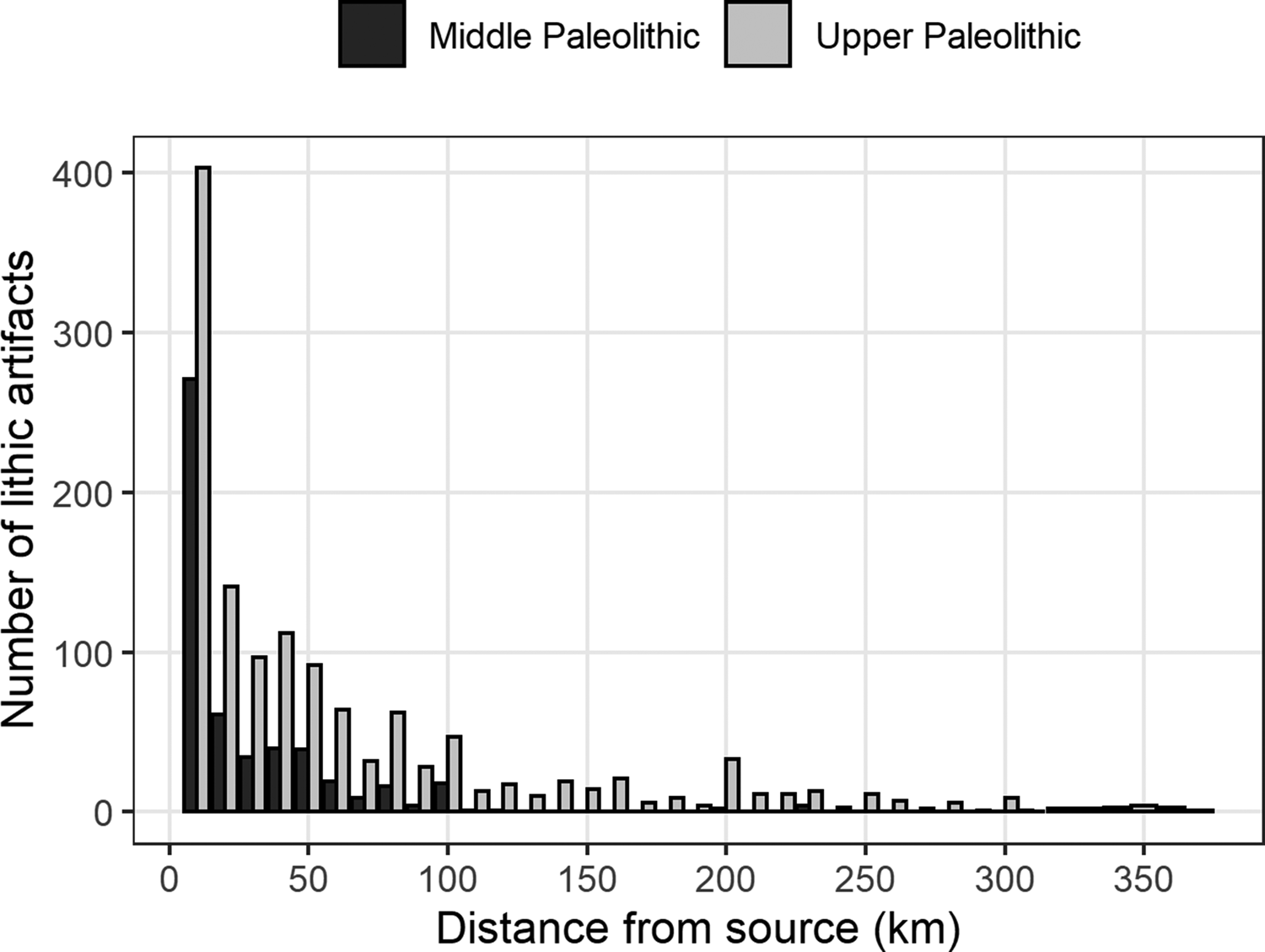
The effect of discard probability is particularly relevant to regions or periods where the timing of the perceived change in the archaeological signal (e.g., distance to source data) coincides to some degree with evidence for a shift in lithic technology. Here we return to interpretations of hominin mobility during the Middle and Upper Paleolithic transition in Europe. Researchers have long speculated that Neanderthals had a smaller lifetime geographic range than modern humans (Mellars Reference Mellars1996). This interpretation is based in part on the observation that many of the Middle Paleolithic stone artifacts that have been sourced were made on local raw materials (often defined as located within 5 or 10 km of the site), with comparatively few examples coming from more distant sources (Figure 7). In comparison, a greater number of sourced Upper Paleolithic stone tools are made on raw material from sources located more than 10 km away, with some artifacts reportedly displaced up to 700 km from their sources. For better or for worse, this purported difference between two archaeological periods—Middle and Upper Paleolithic—has been taken as an indicator of behavioral and/or cognitive differences between two hominin populations—Neanderthals and modern humans. For instance, the apparent focus on local stone types during the Middle Paleolithic is often used as evidence that Neanderthals had a more limited mobility perhaps due to biomechanics and/or myopic land use strategies (Barton et al. Reference Barton, Riel-Salvatore, Anderies and Popescu2011; Steudel-Numbers and Tilkens Reference Steudel-Numbers and Tilkens2004; Verpoorte Reference Verpoorte2006; Weaver and Steudel-Numbers Reference Weaver and Steudel-Numbers2005). On the other hand, the increase in the number of longer-distance transports during the Upper Paleolithic is frequently attributed to a larger geographic range and/or more extensive social network among modern humans (Féblot-Augustins Reference Féblot-Augustins and Pearsall2008), or to a shift toward a predominantly logistical mobility strategy (Barton et al. Reference Barton, Riel-Salvatore, Anderies and Popescu2011; Riel-Salvatore and Barton Reference Riel-Salvatore and Michael Barton2004; but see Premo Reference Premo2012, Reference Premo, Mesoudi and Aoki2015).

Figure 7. Frequency distributions of lithic artifacts by distance to source from a sample of Middle and Upper Paleolithic assemblages in Europe. Note that a single assemblage can contain multiple raw materials with varying distances to their respective sources. Redrawn from data presented in Féblot-Augustins (Reference Féblot-Augustins1999, Reference Féblot-Augustins, Adams and Blades2009).
The simulation results presented here beckon us to reevaluate these interpretations in light of the effects of discard probability. More specifically, the model raises the possibility (which, of course, remains to be tested) that the appearance of more nonlocal raw material in Upper Paleolithic assemblages may have been due to reduced tool discard rather than increased mobility. To attribute the shift in raw material transport solely to a change in mobility, it is necessary to assume that tool discard probability remained constant during the Middle and Upper Paleolithic. This assumption may be difficult to justify given the major difference in lithic technology between the two periods. The Upper Paleolithic witnessed a shift from the flake-based technology of the Middle Paleolithic toward a greater focus on blade/microlithic production. Archaeologists think this signaled an important reorganization in hominin lithic technology that ushered in the more prevalent use of hafted composite tools (Bar-Yosef and Kuhn Reference Bar-Yosef and Kuhn1999). Heavier reliance on hafted tools could mean that Upper Paleolithic hominins were carrying a greater number of smaller stone artifacts in their mobile inventory (Bar-Yosef and Kuhn Reference Bar-Yosef and Kuhn1999; Kuhn Reference Kuhn1994). Moreover, hafted inserts may experience less frequent discard than handheld flake tools because the former tend to get maintained along transit and are only discarded during retooling events at base camps or raw material sources (Keeley Reference Keeley1982). Of course, caution is needed so as not to simply project these functional assumptions onto Paleolithic artifacts, and we do not mean to suggest that this speculation serves as anything more than an interesting alternative hypothesis worth pursuing further. The main point is that given the shift in lithic technology during the Middle-Upper Paleolithic transition, it seems unwise to wholly discount the effects that concomitant changes in discard probability might have had in shaping the distance to source distributions reported for the two periods.
Because the effects of mobility and tool discard are so similar, it is necessary to look to additional independent lines of evidence to disentangle them. Approaches such as Strontium isotope analysis on fossil remains (Moncel et al. Reference Moncel, Fernandes, Willmes, James and Grün2019; Richards et al. Reference Richards, Harvati, Grimes, Smith, Smith, Hublin, Karkanas and Panagopoulou2008) show promise for demonstrating movement of individual hominins relative to different geological regions. Distinguishing the effects of mobility and discard in stone artifacts will be difficult, given that the two variables are interrelated by factors of resource provision, toolkit design, and tool use-life management. Nevertheless, we think there are some testable hypotheses worth pursuing. For instance, raw material sourcing studies have shown that “nonlocal” artifacts during the Middle Paleolithic in Western Europe take a variety of forms—from formal end products to chunks and fragments (Turq et al. Reference Turq, Roebroeks, Bourguignon and Faivre2013). Perhaps this suggests that discard probability did not vary among tool types during the Middle Paleolithic. If raw material was transported more regularly over longer distances during the Upper Paleolithic and if this was related to an increased curation of certain tool forms, such as hafted inserts, rather than to a change in mobility alone, then one might expect different classes of stone tools to display different distance to source distributions. On the other hand, if increased mobility played a greater role, then one might expect to see an increase in distance to source across the board in most stone tool types. Finally, other lithic assemblage measures, such as the cortex ratio, may also help distinguish the relative influence of mobility from discard behavior. In particular, studies have shown that the cortex ratio can be effective for detecting variation in stone artifact transport among assemblages (Dibble et al. Reference Dibble, Schurmans, Iovita and Mclaughlin2005; Lin et al. Reference Lin, McPherron and Dibble2015). It may therefore be possible that the cortex ratio of lithic assemblages responds differently to changes in forager mobility and discard probability. More modeling work, such as that presented by Davies and colleagues (Reference Davies, Holdaway and Fanning2018), is required to evaluate how these assemblage properties vary in relation to the causal processes investigated here.
Critics often question the applicability of neutral models. For example, a common critique of the use of Lévy Walk function for representing human movement is that humans seldom move randomly (Lee et al. Reference Lee, Hong, Kim, Rhee and Chong2008). It is important to clarify that the point of Brantingham's neutral model is neither to replicate exactly how Paleolithic hominins moved nor to elucidate the proximate reasons behind those choices. Instead, the Lévy function is useful because human movement patterns apparently share key characteristics with a Lévy walk distribution—namely, the preponderance of short steps coupled with a heavy tail of longer steps (Baronchelli and Radicchi Reference Baronchelli and Radicchi2013). Given the aggregate and palimpsest nature of the material record, this simple stochastic function provides a convenient and germane way to vary nondirected movement within a controlled setting (Brantingham Reference Brantingham2006). Moreover, current discussions of hominin mobility often assume, either implicitly or explicitly, that the movement patterns of extinct hominins can be effectively summarized using classifications grounded in ethnography, such as the forager-collector continuum (Binford Reference Binford1980). However, it is possible that Pleistocene hominins practiced alternative forms of movement that might not fit neatly into this conceptual model. In this respect, the Lévy walk model offers a useful, flexible alternative to explore mobility patterns outside classic ethnographic examples by capturing general tendencies of human movement using step length and tortuosity (i.e., frequency of turns; see Holdaway and Davies Reference Holdaway and Davies2019).
The relative simplicity of the neutral model also sometimes draws the ire of critics. Indeed, the model presented here is relatively simple and largely “unrealistic”—purposefully so, in fact. To be clear, the purpose of our study is not to replicate the reality of the past (how could one do that when Paleolithic mobility is exactly what we are trying to learn more about?) but rather to investigate the nature of the causal relationships between specific processes and the archaeological landscape systematically (Premo Reference Premo, Costopoulos and Lake2010). A more complex, more “realistic” model might seem more convincing to some, but it would also introduce superfluous and confounding variables to the experiment, making the results more difficult to interpret in terms of cause and effect. Simple models allow for simple experimental designs that are more likely to yield “clean” interpretable results. In many ways, these models are similar to the kinds of controlled experiments that have become more common in lithic studies (Lin et al. Reference Lin, Rezek and Dibble2018; Marreiros et al. Reference Marreiros, Pereira and Iovita2020). Both emphasize variable control and manipulation so that the experimental outcomes can be attributed securely and causally to the experimental variables rather than confounded by “nuisance” factors (Lin et al. Reference Lin, Rezek and Dibble2018). From this perspective, the causal relationships investigated here with a purposefully simple model are certainly relevant to assessing the confidence one places in interpretations that invoke hominin mobility and lithic discard as explanatory factors for distance to source distributions in the archaeological record.
However, our emphasis on simplicity and our focus on an experimental design tailored to address the effect of discard probability does not mean that all the processes excluded from this model are (or were) unimportant. Indeed, the relative effects of other potentially influential factors should be systematically explored before they are integrated into a larger, more complex model. For example, although a Lévy walk may be an optimal strategy for “blind foragers” searching for sparse and unevenly distributed resources (Humphries and Sims Reference Humphries and Sims2014), studies have emphasized the important role that spatial memory plays in human and nonhuman animal movement (Fagan et al. Reference Fagan, Lewis, Auger-Méthé, Avgar, Benhamou, Breed and Ladage2013). Put simply, humans are shown to have a strong propensity to return to locations they have visited previously. One consequence is that newly explored locations are commonly concentrated around previously visited “hot spots” (Lee et al. Reference Lee, Hong, Kim, Rhee and Chong2008; Song et al. Reference Song, Koren, Wang and Barabási2010). Frequently visited locales can correspond to the locations of key resources (e.g., fresh water sources) or the presence of certain geographic features (e.g., higher ground or shelters). In the presence of spatial memory, such natural resources act as “attractors” for persistent human activities (Davies Reference Davies2016; Haas and Kuhn Reference Haas and Kuhn2019; Reeves Reference Reeves2019). From a paleoanthropological perspective, these additional parameters—particularly spatial memory and the reuse of certain spaces—are especially interesting to explore with respect to discussions of information transmission and cumulative culture in human evolution (Henshilwood and Marean Reference Henshilwood and Marean2003). By integrating these aspects into a Lévy-based movement model, it may be possible to develop a formal means to test for the timing of cumulative information sharing using archaeological data (Perreault and Brantingham Reference Perreault and Jeffrey Brantingham2011).
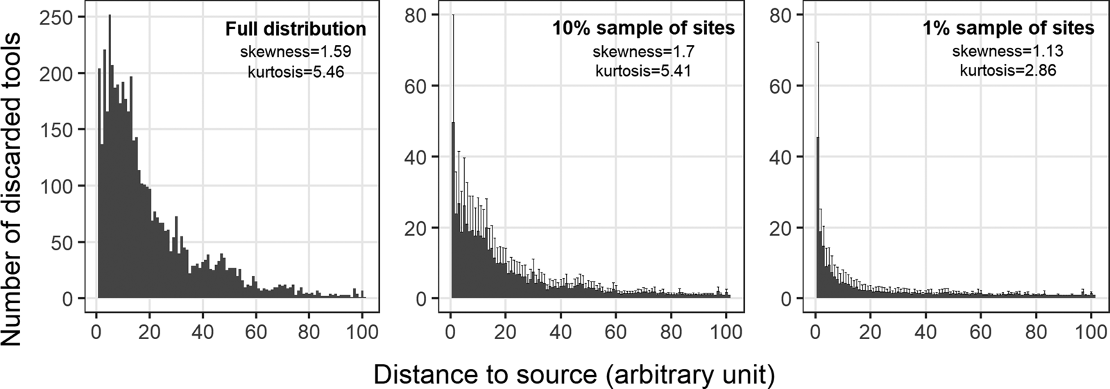
We also need more explicit testing of the ways that differential preservation and sampling can affect what are too often merely presumed to be behavior-caused patterns in archaeological landscapes. For example, recent modeling efforts have shown how geomorphic processes such as sedimentation and erosion can alter the availability and accessibility of previously discarded materials to subsequent foragers (Davies and Holdaway Reference Davies and Holdaway2018; Davies et al. Reference Davies, Holdaway and Fanning2016). But sampling artifacts by site may present an even bigger issue for the case of raw material transport. Given that one's sample of the underlying landscape of artifacts is almost always structured by “site” and that the underlying distribution of number of discard sites by distance to source is very likely to be right skewed (Figure 2), the shape of any empirical distance to source distribution can vary considerably due to sampling variation in number of discard sites alone. To illustrate this basic but subtle point briefly, we first create 1,000 distance to source distributions composed of artifacts collected from a random sample of 10% (and then 1,000 more from a random sample of 1%) of the total number of discard sites from one of our simulation runs (μ = 2.0 and λ = 0.9) (center and right panels in Figure 8). We then use the two-sample Kolmogorov-Smirnov test to compare each of these samples to a distance to source distribution created by randomly sampling a comparable number of artifacts from the archaeological landscape at large—that is, in this case, we sample the “full” distribution of artifacts without respect to discard site (left panel in Figure 8). The former sampling design approximates how archaeologists often conduct landscape-scale studies with aggregated site datasets (e.g., Féblot-Augustins Reference Féblot-Augustins, Adams and Blades2009), whereas the latter represents the kind of truly random sampling of artifacts in a region's archaeological record that can rarely be done given the realities of archaeological fieldwork. A test outcome with p < 0.05 would suggest that the two samples were derived from different populations. Because all samples were taken from the same archaeological landscape, one would expect approximately 5% of the Kolmogorov-Smirnov tests to yield p < 0.05 if randomly sampling by discard site—rather than by artifact—has no effect on the distance to source distribution. However, the observed proportions of statistically significant tests are an order of magnitude greater than expected. For samples collected from 10% of the discard sites, 50.6% of 1,000 Kolmogorov-Smirnov tests yield p < 0.05, and for samples collected from 1% of the discard sites, 45.8% of 1,000 Kolmogorov-Smirnov tests yield p < 0.05. As this resampling exercise illustrates, the distance to source values associated with artifacts collected from a random sample of discard sites are not necessarily “representative” of the underlying archaeological landscape. In fact, when compared to the distance to source distributions of artifacts drawn from the landscape at large, the distance to source distributions associated with artifacts collected from just 10% or 1% of the discard sites regularly differ in ways that would be interpreted as reflecting a decidedly more “local” mobility strategy, despite the fact that all samples were taken from the same archaeological landscape.

Figure 8. When dealing with a right-skewed distance to source distribution, sampling the archaeological landscape by “site” introduces a systematic bias whereby decreasing the number of discard sites in one's sample yields a distance to source distribution that looks significantly more “local”: (left) number of artifacts by distance to source in the archaeological landscape generated by a single simulation run (μ = 2.0 and λ = 0.9)—this particular archaeological landscape contains 5,000 artifacts distributed over 2,179 discard sites; (center) the mean (and 1 standard deviation) number of artifacts per distance to source from 1,000 random samples, each of which contains artifacts collected from just 10% of the discard sites from the same simulation run depicted in the left panel; (right) the mean (and 1 standard deviation) number of artifacts per distance to source from 1,000 random samples, each of which contains artifacts collected from just 1% of the discard sites from the same simulation run depicted in the left panel. Note that the scale of the y-axis varies among panels, and the x-axis is truncated at 100 to aid with illustration.
And it is not just variation in the number of discard sites sampled that can distort one's view of the actual distance to source distribution. Variation in the number of artifacts recovered from each assemblage introduces a second source of sampling bias. Because artifacts made on nonlocal raw materials tend to be rarer than those made on local raw material within every lithic assemblage, archaeologists’ ability to document long-distance raw material transport is also heavily dependent on the number of artifacts recovered from an assemblage (Hiscock Reference Hiscock2001). The maximum distance to source of each assemblage is especially sensitive to sample size simply because maximum distance depends on recovering at least one example of what are often the lowest-density occurrences in all Paleolithic stone tool assemblages—tools made of raw material transported over a great distance (Féblot-Augustins Reference Féblot-Augustins, Adams and Blades2009). Here, variation in the size of the samples obtained from assemblages alone can systematically bias the distance to source distribution in such a way that assemblages from which a smaller number of artifacts are collected (or sourced) consistently show a more “local” signal than assemblages from which a larger number of artifacts are studied, even if there was no difference in past mobility, discard probability, or the size of the assemblages in the ground. One relatively simple and straightforward way to quantify the extent to which the distance to source distributions associated with the Middle and Upper Paleolithic in Europe are affected by this second type of sampling bias is to test for the effect of “assemblage size” (i.e., the number of artifacts collected from each assemblage)—or even better, the number of tools that have been sourced from each assemblage—on measures such as the number of tools made on nonlocal raw material per assemblage and the maximum distance to source per assemblage. We summarize the implications of the potential effects of sampling bias on right-skewed archaeological distance to source distributions as follows: if the number of Middle Paleolithic sites sampled is lower than the number of Upper Paleolithic sites sampled, if the number of tools recovered per Middle Paleolithic assemblage is lower than the number of tools recovered per Upper Paleolithic assemblage, and/or if Middle Paleolithic assemblages are associated with fewer “sourced” tools on average than Upper Paleolithic assemblages so that sampling variation alone can explain the aforementioned differences between the two periods’ distance to source data (Figure 7), then there may be no need to offer behavioral explanations that posit changes in hominin mobility or discard probability.
Conclusion
Reconfirming the conclusion of Brantingham (Reference Brantingham2003, Reference Brantingham2006), the decay-like distance to source distribution commonly observed in archaeological data emerges from the interaction between nondirected hominin movement and discard probability. Our results do not “prove” that Paleolithic hominins moved according to a random walk or that they did not prefer some raw materials over others. However, our controlled experiment demonstrates that it is difficult to retrospectively identify the relative effects of mobility and discard due to their similar effects on distance to source data. Because similar archaeological patterns can result from changes in mobility or discard probability—or both—one should be cautious about inferring large-scale changes in hominin mobility and land use based on relatively subtle shifts in distance to source distributions without first ruling out concomitant changes in stone tool technology that would affect discard probability. Researchers will need to consider multiple lines of evidence to discern the respective roles that changes in mobility and discard behavior may have played in the formation of Paleolithic archaeological landscapes.
Archaeologists are no strangers to equifinality or to the challenges it poses. Archaeologists often rely on “verbal logic” (Servedio et al. Reference Servedio, Brandvain, Dhole, Fitzpatrick, Goldberg, Stern, Van Cleve and Justin Yeh2014) when choosing among the many potential explanatory variables that deserve attention. This seems a fine place to start but a bad place to end. A model-based approach provides the framework necessary for testing hypotheses generated by verbal logic (or by ethnographic observation) for formally assessing whether there is in fact a unique causal relationship between the proposed behavioral process and an archaeological pattern of interest. It is important to note that the aim of this modeling approach is not to provide realistic reconstructions of past hominin land-use systems but rather to systematically explore and evaluate explicitly stated research questions regarding a hypothesized cause-and-effect relationship between behavior (e.g., mobility, discard probability, etc.) and archaeological signal (e.g., maximum distance to source). We believe this basic but fundamental work is best served by simple models and clean experimental designs. We hope that, bit by bit, we will be able to build our understanding of how various human and natural processes affect the formation of archaeological landscapes. In this vein, our study provides a tiny piece to a much larger puzzle by showing the relative influences of forager mobility and discard probability on distance to source data. Much like Brantingham's original Lévy walk model, we view this study as another case in which a relatively simple model serves to remind us of just how complicated and difficult it is to infer behavior from archaeological assemblages.
Acknowledgments
This study was supported by the Australian Research Council (DE200100502) and the Department of Human Evolution, Max Planck Institute for Evolutionary Anthropology. Benjamin Davies, Alex Mackay, and two anonymous reviewers offered valuable comments on earlier drafts that helped improve the article. We thank Maria Esteban Palma for her assistance with the Spanish abstract translation.
Data Availability Statement
The fully commented NetLogo source code, full model description, data, and the R code used to generate the graphics are available at https://doi.org/10.5281/zenodo.5035823.
Supplemental Material
For supplemental material accompanying this article, visit https://doi.org/10.1017/aaq.2021.66.
Supplemental Table 1. Summary of the Mean Step Length and Total Time Steps per Simulation Run (mean and 2.5th–97.5th percentile range). Each cell in the table summarizes data collected from 50 simulation runs at each combination of μ and λ. For mean step length, the data presented here are the mean and percentile range of the mean step length per simulation. Note that λ does not affect mean step length when controlling for μ. Also note that μ does not affect time steps per simulation run when controlling for λ.