


Introduction
Recently, physiological methods have been used in the study and understanding of design protocols, the design process, and design cognition. These methods include eye-tracking (Kahneman, Reference Kahneman1973) and gesture analysis (Tang & Zeng, Reference Tang and Zeng2009), galvanic skin response (GSR) (Nguyen & Zeng, Reference Nguyen and Zeng2016), electrocardiograms (ECG) (Moriguchi et al., Reference Moriguchi, Otsuka, Kohara, Mikami, Katahira, Tsunetoshi, Higashimori, Ohishi, Yo and Ogihara1992; Nguyen & Zeng, Reference Nguyen and Zeng2014), and electroencephalograms (EEG) (Alexiou et al., Reference Alexiou, Zamenopoulos, Johnson and Gilbert2009; Nguyen & Zeng, Reference Nguyen and Zeng2010, Reference Nguyen and Zeng2012). Medical and physiological apparatuses have become more widespread, non-invasive (perhaps even ubiquitous), user-friendly and accessible. Some recent advances are to be found in (Nguyen & Zeng, Reference Nguyen and Zeng2010, Reference Nguyen and Zeng2016; Goel, Reference Goel2014; Goel et al., Reference Goel, Eimontaite, Goel and Schindler2015; Jaarsveld et al., Reference Jaarsveld, Fink, Rinner, Schwab, Benedek and Lachmann2015). Currently, the most popular technique for design protocol analysis is the verbal protocol. However, verbal protocols are known to suffer from limitations (Chiu & Shu, Reference Chiu and Shu2010). This is especially true when dealing with nonreportable processes such as creative tasks, insight, effective judgment, task parallelism or automated tasks (Kuusela & Paul, Reference Kuusela and Paul2000). Irmscher (Reference Irmscher1987) argues that researchers should disrupt as little as possible “the natural setting”. It then follows that other techniques for protocol analysis should be investigated.
In our previous work (Nguyen et al., Reference Nguyen, Nguyen and Zeng2015), we have shown how an EEG-based segmentation algorithm can emulate basic protocol segmentation. We have shown how it can provide valuable insight on hidden cognitive features. The segmentation algorithm was based on transient microstates (as a correlate to mental effort). It was also based on the heuristic that different tasks engage different levels of mental effort. The heuristic also incurred the known risk that two successive tasks engage the same level of mental effort. Transient microstates are short duration microstates that rapidly change to another scalp field configuration. In this paper, we extend this method to include other EEG features (e.g. spatio-temporal and frequency domain). These measure various mental states (e.g. mental effort, fatigue, and concentration). The EEG features we use to measure mental states constitute the protocol encoding. The EEG-based segmentation algorithm provides the protocol segmentation. We compare the manual segmentation of a set of design protocols recorded on a touchpad provided by domain experts with various EEG-based segmentations. Our method is fully automated. We argue that it provides an insight into cognitive processes that are often left unseen by traditional protocol analysis methods. Our method does not replace traditional protocol analysis, but rather complements it. We argue that EEG-based segmentation is a feasible method.
Advantages of such a method are as follows. EEG segmentation is fully automated and can be readily included in engineering systems and subsystems. It is hands-free and non-intrusive (using commercial modern EEG technologies). It allows the researcher to detect cognitive processes that would otherwise be invisible to him (i.e. when verbal protocols fail).
Disadvantages of such a method are as follows. EEG segmentation does not replace traditional verbal protocols, especially in the case of complex protocol segmentations. It rather serves as a complement to these techniques. EEG-based segmentation may sometimes yield segments that are hard to interpret as the cognitive processes may be hidden. For example, EEG signals are noisy in nature and require preprocessing using noise and artifact removal techniques.
The scope of our research is to demonstrate a biometric signal-based method to perform simple design protocol segmentation. Furthermore, we provide comparisons with segmentations performed by human domain experts.
The rest of this paper is organized as follows. Section “Verbal protocols: strengths and weaknesses” reviews the strengths and weaknesses of verbal protocol analysis. Section “The experimental data” describes the design protocol data based on our analysis and experiments. Section “A physiological method for design protocol segmentation” describes a fully physiologically based segmentation technique using EEG. More specifically, the notion of functional microstates of the brain is discussed. The data used in the experiments come from a set of experiments performed over the past years at the Design Lab. Subjects were asked to perform various design tasks while having their EEG monitored. Section “Comparions between techniques” provides experimental validation and analysis of different EEG-based segmentation methods. In particular, we compare design protocol segmentations manually done by domain experts and different EEG-based methods (transient microstates and power spectral densities).
Verbal protocols: strengths and weaknesses
Verbal protocols have been widely used by design researchers to understand cognitive aspects of the conceptual design process since the work of Ericsson & Simon (Reference Ericsson and Simon1984). They have been used in design research in (Enis & Gyeszly, Reference Enis and Gyeszly1987; Cross et al., Reference Cross, Christiaans, Dorst, Cross, Christiaans and Dorst1996; Gero & McNeill, Reference Gero and McNeill1998; McNeill et al., Reference McNeill, Gero and Warren1998). A few techniques can be found in the literature on the subject: concurrent verbalization, direct reports, informal reporting and retrospective protocol analysis. Concurrent verbalization (i.e. simultaneous) is often contrasted with retrospective protocol analysis (i.e. post-hoc). In design research, concurrent verbalization is the most popular method to study design cognition (Jiang & Yen, Reference Jiang and Yen2009). Protocol encoding and segmentation are discussed from the perspective of design protocol analysis in (Enis & Gyeszly, Reference Enis and Gyeszly1987; Ullman et al., Reference Ullman, Stauffer and Dietterich1987; Gero & McNeill, Reference Gero and McNeill1998; McNeill et al., Reference McNeill, Gero and Warren1998; Kan & Gero, Reference Kan and Gero2008; Stacey et al., Reference Stacey, Eckert, Earl, McDonnell and Lloyd2009). Akin (Reference Akin, McDonnell and Lloyd2009) discusses an encoding of a design protocol involving architects to test the hypothesis that architects design by operating breadth-first and depth-next. Dong et al. (Reference Dong, Kleinsmann, Valkenburg, McDonnell and Lloyd2009) encode a design protocol to detect appraisal based on linguistic coding strategies. Ball and Christensen (Reference Ball, Christensen, McDonnell and Lloyd2009) propose the use of hedge words such as “like” to detect analogical thinking, “I think” to detect mental simulation and “I guess” or “sort of” to detect uncertainty. These hedge words are then used to encode the design protocol. Another example comes from Dantec & Do (Reference Dantec, Do, McDonnell and Lloyd2009). Mechanisms of valuation are studied by encoding the protocol data into concepts. These concepts were design values (form, material, aesthetic), human values (spirituality, respect, family), requirements, narrative and processes. Different participants of the design protocol are then measured against their use of these concepts. This is used to determine levels of value transfers occurring in the design protocol. Conversation-analytic methods such as interruptions and unfinished turns delineation have also been used in Matthews (Reference Matthews, McDonnell and Lloyd2009) to detect social order among participants. Automated tagging of design protocols was studied in Rosé et al. (Reference Rosé, Wang, Cui, Arguello, Stegmann, Weinberger and Fisher2008) using automated text classification and machine learning techniques. Features are computed over text segments such as unigrams and bigrams, stems and rare words. Textual protocol data sets lend themselves well to ontology learning and knowledge discovery techniques (Völker et al., Reference Völker, Hitzler and Cimiano2012; Wong et al., Reference Wong, Lieu and Bennamoun2012). More complex techniques for design protocol analysis exist such as the Function-Behavior-Structure ontology (Gero, Reference Gero1990; Kan & Gero, Reference Kan and Gero2008) and linkography (Kan & Gero, Reference Kan, Gero, McDonnell and Lloyd2009). The latter allows for collaborative protocol analysis.
Kuusela and Paul (Reference Kuusela and Paul2000) argue that concurrent verbalization techniques are more complete (i.e. measured as the number of protocol segments) than retrospective protocol analysis. However, the latter gains by not interfering in the conceptual design process. Furthermore, retrospective protocol analysis suffers from post-hoc imprecision. The quality of verbal protocols is known to decrease (i.e. no longer describe a cognitive process) as the memory of a task leaves a subject's short-term memory (Ericsson & Simon, Reference Ericsson and Simon1984). In the design literature, domain experts often perform encodings manually. More than one domain expert is also often used to alleviate subjective ratings. In some cases, the same person performs encoding, but each encoding session is separated by a time lag (Kan & Gero, Reference Kan, Gero, McDonnell and Lloyd2009).
Verbal protocols are known to bear some weaknesses. Wilson (Reference Wilson1984) and Kuusela and Paul (Reference Kuusela and Paul2000) note that verbal protocol does not trace cognitive processes that are not part of “focal attention”, such as “subliminal stimulus” (i.e. “subliminal primes”). Furthermore, they do not trace thoughts that do not reach the verbalization process. Furthermore, Wilson (Reference Wilson1984) argues that concurrent verbalization changes the sequence of thought processes (i.e. “the reactive effects of verbal protocol”). Schooler et al. (Reference Schooler, Ohlsson and Brooks1993) run four sets of experiments to show that verbalization interferes with problem-solving. They show that subjects asked to verbalize their problem-solving strategies were significantly less successful than control subjects. Wilson et al. (Reference Wilson, Lisle, Schooler, Hodges, Klaaren and Lafleur2013), Schooler et al. (Reference Schooler, Ohlsson and Brooks1993), Fallshore and Schooler (Reference Fallshore and Schooler1993), Wilson and Schooler (Reference Wilson and Schooler1991), Schooler et al. (Reference Schooler, Ryan and Reder1991), and Schooler and Engstler-Schooler (Reference Schooler and Engstler-Schooler1993) all argue that verbalization affects performance. Schooler et al. (Reference Schooler, Ohlsson and Brooks1993) state that “certain thoughts have a distinctly nonverbal character” such as creative thoughts and insights (i.e. unexpected problem solutions that just happen). Furthermore, the authors study facial recognition as an example of a task that requires large amounts of information that cannot be easily verbalized (Schooler et al., Reference Schooler, Ohlsson and Brooks1993). Creativity and insight are then argued to “have occurred in the absence of words” (Schooler et al., Reference Schooler, Ohlsson and Brooks1993). Wilson and Schooler (Reference Wilson and Schooler1991) discuss how verbalization increases the salience of verbal attributes and “overshadows” nonverbal attributes (e.g. effective judgment is often ignored using verbalization). Verbal overshadowing was then defined as a subject's focus on verbally relevant information to the detriment of information that is not easily verbalized. The subjectivity of verbal protocols (e.g. self-presentational concerns) is also discussed in Wilson (Reference Wilson1984). Fabrication problems in design protocols are discussed in Kuusela & Paul (Reference Kuusela and Paul2000). Smagorinsky (Reference Smagorinsky1989) also reports that subjects have a hard time verbalizing while manipulating objects. Chiu and Shu (Reference Chiu and Shu2010) argue that verbal protocols showed limitations in their experiments by contradicting the assumption that stimuli increase concept creativity. The authors then raise three concerns related to verbal protocols: time and resource intensiveness (i.e. the technical setup of verbal protocols), data validity, and the fact that some tasks are not conducive to verbalization. For example, task parallelism impacts verbalization (which is inherently sequential) and automaticity (Rasmussen & Jensen, Reference Rasmussen and Jensen1991; Gordon, Reference Gordon1992). Schooler et al. (Reference Schooler, Ohlsson and Brooks1993) and Metcalfe (Reference Metcalfe1986) note that in the context of insight problem solving, “subjects who believe that a solution is imminent are engaging in a ‘gradual rationalization process’ that focuses them on an inaccurate yet reportable approach”. Schooler et al. (Reference Schooler, Ohlsson and Brooks1993) listed few types of insight problem-solving tasks as follows: memory retrieval tasks, spreading activation tasks (i.e. how the brain navigates in a network of thoughts), constraint relaxation (i.e. how we remove a constraint on a problem that is false) and perceptual reorganization (e.g. Necker cube illusion). They form a group of “difficult-to-report perceptual and memory processes” (Schooler et al., Reference Schooler, Ohlsson and Brooks1993). Ericsson and Simon (Reference Ericsson and Simon1984) argue that concurrent verbalization is qualitatively correct while only decreasing the overall performance of problem-solving. On the other hand, Schooler et al. (Reference Schooler, Ohlsson and Brooks1993) argue that in the case of insight problem-solving, verbalization impedes cognitive processes as it “overshadows” nonreportable processes. This latter approach is clearly gestaltist.
When hidden cognitive processes are of concern, Wilson (Reference Wilson1984) concludes that verbal protocols cannot be “taken on faith”. There are some tasks where verbal protocols yield poor quality results such as creative tasks, insight (e.g. the “Aha” experience, gestalt psychology), effective judgment, memory retrieval tasks, task parallelism or automated tasks (e.g. facial recognition, visual recognition tasks). These tasks are sometimes termed as nonreportable processes (Schooler et al., Reference Schooler, Ohlsson and Brooks1993). More specifically, Wilson (Reference Wilson1984) argues that while verbal protocols are not “completely invalid”, they do not provide “a perfect window into the mind”. By doing so, the author challenges the positions long held in Ericsson & Simon (Reference Ericsson and Simon1984) where it is believed that research has “overestimated the extent of nonconscious processing”.
The weaknesses of verbal protocols are one of the main reason why alternative techniques based on sketching (Suwa & Twersky, Reference Suwa and Twersky1997), kinesics (Tang & Zeng, Reference Tang and Zeng2009), electrocardiograms (Moriguchi et al., Reference Moriguchi, Otsuka, Kohara, Mikami, Katahira, Tsunetoshi, Higashimori, Ohishi, Yo and Ogihara1992), gesture analysis (Visser, Reference Visser, McDonnell and Lloyd2008), and eye-tracking (Kahneman, Reference Kahneman1973) have been researched.
The experimental data
The Design Lab gathered over the past few years datasets of subjects performing various design tasks while having their EEGs monitored and their actions recorded on a touchpad (Nguyen & Zeng, Reference Nguyen and Zeng2010, Reference Nguyen and Zeng2012, Reference Nguyen and Zeng2014). We used a subset of eight datasets recorded on eight different subjects to perform our experiments. We chose these datasets because the quality of the EEG recordings was higher. Although the number of subjects was low, the quantity of data gathered was high as each design episode lasted up to 2 h. The questions that the subjects were asked to solve on the touchpad were the following (cf. Figure 1):
• Make a birthday cake for a 5-year-old kid. How should it look like?
• Sometimes, we do not know which items should be recycled. Create a recycle bin that helps people recycle correctly.
• Create a toothbrush that incorporates toothpaste.
• In many cities, people in wheelchairs cannot use the metro safely because most metros only have stairs or escalators. Elevators are not an option because they are costly. You are asked to create an effective solution to solve this problem.
• Employees in IT companies sit too much. The company wants their employees to stay healthy and work efficiently at the same time. You are asked to create a workspace that can help employees to work and exercise at the same time.
• There are two problems with standard drinking fountains: (a) filling up water bottles is not easy, (b) short people cannot use the fountain and tall people have to bend over. Create a new drinking fountain that solves these problems.
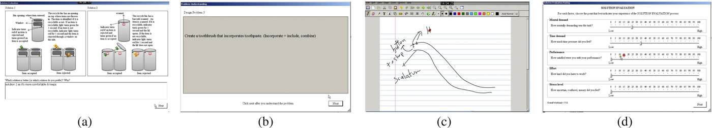
Fig. 1. (a) Displays a typical answer multiple choice question segment, (b) a read question segment, (c) a sketch segment, and (d) a rate problem segment [we used NASA-TLX (NASA, 1986)]
Each problem was composed of three subtasks: (1) sketch a solution for the problem; (2) to choose the best design between two proposed designs (the proposed design were either taken from existing designs in the literature or created by us); (3) rate the hardness of the problem using NASA-TLX (NASA, 1986). Among the proposed designs, those taken from the literature were the cake, the escalator, the drinking fountain (one of the proposed solutions), and the exercise at workplace problems; those created by us were the toothbrush, the drinking fountain (one of the proposed solutions), and the recycle bins problems.
The resolution by a subject of all six problems constituted the design session which lasted between 30 min to 2 h depending on the subjects. Each task lasted about 1–10 min. During the design sessions, we gathered EEG signals of length between 1,000,000 and 4,000,000 samples. Although the number of subjects in our experiments was low, the data gathered were large enough to account for within-subject variations. Each subject was asked to solve all questions, which increased the reliability of our data. If we count eight subjects, six problems per subject and three tasks per problem (sketch, choose, rate), we have a total of 144 tasks. The Human Research Ethics and Compliance of our university approved our experimental protocol. Subjects volunteered to participate in the experiments. Subject selection was randomized and no gender considerations were used. All subjects were graduate students from the Quality System Engineering program at our university. The ages of subjects ranged from 25 to 35. The best design was rewarded with a 100$ gift card as an incentive.
A physiological method for design protocol segmentation
EEG was invented by H. Berger in 1937 who described it as a window into the brain (Michel et al., Reference Michel, Koenig, Brandeis, Gianotti and Wackermann2009). EEGs are the potential values of a scalp field map. Many methods exist to analyze EEG raw data. Among them are frequency-domain techniques such as power spectral densities (PSD) (Michel et al., Reference Michel, Koenig, Brandeis, Gianotti and Wackermann2009), and spatio-temporal techniques such as functional microstate analysis (Pascual-Marqui et al., Reference Pascual-Marqui, Michel and Lehmann1995; Blankertz et al., Reference Blankertz, Tangermann, Vidaurre, Dickhaus, Sannelli, Popescu, Fazli, Danczy, Curio, Müller, Graimann, Allison and Pfurtscheller2010).
Functional microstates of the brain
Many methods exist to segment EEG data: some of them are frequency-based such as power spectral densities and others are spatio-temporal. Microstate analysis forms a set of spatio-temporal techniques that apply to multichannel EEG recordings. Microstates are features of an EEG epoch extracted using clustering-like methods. Microstates are sub-second quasi-stable configurations of scalp field map potential values that quickly change to another quasi-stable configuration. It makes sense to cluster the scalp field maps into representative cluster centroids. Experimentally, this number of representative cluster centroids was found to be 4 on subjects with eyes closed (Pascual-Marqui et al., Reference Pascual-Marqui, Michel and Lehmann1995). Blankertz et al. (Reference Blankertz, Tangermann, Vidaurre, Dickhaus, Sannelli, Popescu, Fazli, Danczy, Curio, Müller, Graimann, Allison and Pfurtscheller2010) propose different machine learning techniques to obtain these centroids. Pascual-Marqui et al. (Reference Pascual-Marqui, Michel and Lehmann1995) propose the P2ML algorithm, an optimized clustering technique based on eigenvalues and Lagrangians. The squared orthogonal distance between different scalp field maps is used. The objective function then finds the patterns that are closest to some cluster centroids. The cluster centroids are initially guessed and iteratively set to converge to an optimum. This optimum may be a local optimum and may not be a global optimum. Using the P2ML algorithm, the strength of the system's eigenvalues can be used to estimate the number of required cluster centroids. The strength of the eigenvalues then measures the number of eigenvectors needed to represent the system.
Given an EEG signal, a global power field curve can be computed. Each point on the global field curve corresponds to a sample. The sample then corresponds to a scalp field map. This is shown in Figure 2. The theory of functional microstates states that these scalp fields are stable for subsecond periods and that these stable configurations reoccur. This means that the scalp field maps of an EEG signal can be clustered into representative centroids. These centroids can then provide a means to segment an EEG signal.

Fig. 2. Segmentation of an EEG signal using the P2ML algorithm (left) and smoothed segmentation using the regularized P2ML algorithm (right). The microstates to which each segment is related are shown above and below
The P2ML algorithms: an outline
The P2ML algorithm allows for the clustering of EEG scalp field maps. The clustering then allows for the segmentation of the EEG signal into microstates. The P2ML algorithm also allows for the smoothing of the segmentation. Given an EEG signal of 12 samples, the segmentation of the EEG according to microstates 1, 2, 3, and 4 may be: (1, 1, 1, 1, 3, 3, 3, 2, 4, 4, 4, 4). The eighth sample is segmented to microstate 2 but has a short duration of only one sample. This microstate is a transient microstate. A transient microstate is a short-duration microstate that rapidly changes to another scalp field configuration. An important physiological metric brought forth by the concept of microstates is the duration of the microstates. The number of transient microstates is an important characteristic of the functional microstate segmentation. The P2ML algorithm has a regularized version. This version allows the generation of a smoothed segmentation in which transient microstates incur a smoothness penalty. The regularized segmentation of our example could then be: (1, 1, 1, 1, 3, 3, 3, 3, 4, 4, 4, 4). Figure 2(left) shows the segmentation of a global field power curve into 4 microstates. The P2ML algorithm computed 35 segments. Figure 2(right) shows the segmentation of the same global field power curve using the regularized P2ML algorithm and 4 microstates. The regularized P2ML algorithm computed 21 segments.
In practice, the P2ML objective function is given for a set of k candidate microstates M k and electric potential values V t at time t as:
 $$\arg \,\mathop {\max} \limits_{\rm k} \{ (V_{\rm t} \cdot M_{\rm k})^2\} $$
Using vector geometry, it can be shown that the orthogonal squared distance between V t and M k is given by (Freudiger, Reference Freudiger2003):
 $$d^2(V_{\rm t}\comma \,M_{\rm k}) = (V_{\rm t} \cdot V_{\rm t}) - (V_{\rm t} \cdot M_{\rm k})^2$$
By maximizing the second term of the equation (V t · M k)2, we are effectively minimizing the orthogonal squared distance between V t and M 1,…, M k,…
The regularized objective function of the P2ML algorithm is given for a set of k candidate microstates M k and electric potential values V t at time t as follows. It outputs the smoothed segmentation:
 $$\arg \,\mathop {\min} \limits_k \left\{ {\displaystyle{{(V_t \cdot V_t) - {(V_t \cdot M_k)}^2} \over {2e(N - 1)}} - \lambda E} \right\}\comma \,$$
where λ is a smoothness penalty coefficient and E is a smoothness penalty function given by:
 $$E = \sum\limits_{i = t - w}^{t + w} {\delta \lpar {S_i\comma \,n} \rpar \comma \,\quad} n = 1\comma \,{\rm \ldots}\comma \, k$$
for a segment number S i (the numerical index k of the microstate M k) and a delta function given by:
 $$\delta (x\comma \,y) = \left\{ {\matrix{ {1\comma \,} & {x = y\comma \,} \cr {0\comma \,} & {\hbox{otherwise}{\rm.}} \cr}} \right.$$
The parameter e is a measure of the average distance between the data and the microstates. The smoothness penalty λE increases when contiguous segments are clustered to the same microstate. It decreases when contiguous segments are different on some window size parameter is given by w. The overall objective function then decreases when the segmentation is smooth. It increases when the segmentation is non-smooth. Transient segments are then penalized and removed accordingly by the algorithm.
To estimate the number of microstates used in the clustering algorithm, the P2ML algorithm uses the number of significant eigenvalues/vectors in the system. The number of significant values in the eigensystem corresponds to the number of components necessary to explain the system's overall variance. For a subject with eyes closed, this number has been found to be typically 4 (Lehmann et al., Reference Lehmann, Ozaki and Pal1987; Pascual-Marqui et al., Reference Pascual-Marqui, Michel and Lehmann1995).
Frequency-domain features
Power spectral densities are computed over specific frequency ranges of an EEG signal. It is, therefore, a frequency-domain feature. The frequency ranges usually used in EEG analysis are the alpha band (range), beta band (range), delta band (range), and theta band (range). Other frequency ranges also exist such as gamma (somatosensory cortex) and mu bands (sensorimotor cortex). Combinations of these frequency bands are often used to compute such characteristics as fatigue, concentration, and attention.
Many techniques exist to approximate PSD such as correlogram and periodograms. Here, we use the modulus of the Discrete Fourier Transform (DFT) of a given sample x within a specific frequency range as follows:
 $$PSD_{{\rm range}} = \sum\limits_{\tau \in {\rm range}} {\vert {DFT_\tau (x)} \vert }. $$
This effectively yields the power of a signal within a given frequency range.
For example, if the modulus of the DFT of a signal is given by (1, 2, 2, 3, 5, 2, 1, 4, 5, 63, 2) and the associated frequencies are in the range 1–12 with 1 Hz units, computing the 3–4 Hz frequency range is done by summing 2 + 3 = 5 Hz.
The PSD is a widely used feature of EEG signals, if not the most widely used. It is effectively used to detect eye-blinking artifacts, sensorimotor artifacts, sleep cycles, and other states of mind such as fatigue, concentration, and relaxation. The PSD is usually computed on a given electrode of a multichannel EEG such as FP1 (left frontal area).
Physiologically-based segmentation using transient microstates and PSD
While the P2ML and PSD algorithms effectively segment an EEG into microstates, the segmentation is not usable in the context of design protocol data segmentation. It is too fine-grained and its application pertains to electrical neuroimaging. We have built an analysis layer over the P2ML and PSD algorithms to effectively segment design protocol data in a manner that makes sense in design studies. We used the heuristic that the perceived and evoked transient percentage of two different subtasks is different. To measure this evoked transient percentage, we have used the P2ML algorithm.
The measure we use to quantify and valuate subtasks of a design protocol dataset as measured by an EEG signal is the transient microstate percentage. The transient microstate percentage (TM%) is given by:
 $$TM\% = \displaystyle{{Segments - SmoothSegments} \over N}$$
The transient microstate percentage measures the percentage of microstates that were transient. In the equation, the number of discontinuous segments obtained using the P2ML algorithm gives the number of segments. The number of segments obtained using the regularized P2ML algorithm gives the number of “smooth segments”. This works because the number of “smooth segments” computed using the regularized P2ML algorithm does not account for transient microstates (short duration microstates). For example, the segmentation (1, 1, 1, 2, 2, 3, 4, 1) has five discontinuous segments. In Figure 2(left), the P2ML segmentation has 35 discontinuous segments while the regularized P2ML segmentation in Figure 2(right) has 21 discontinuous segments. The difference between both values gives a transient microstate valuation of 14. Since the number of samples is 200, the transient microstate percentage is 0.07.
The transient microstate percentage effectively measures the percentage of short duration microstates with respect to the total number of samples in the signal. This number is always positive and smaller than 1. Transient microstates are deemed to be a significant metric in EEG signal processing and were characterized as being the atoms of thought (Lehmann, Reference Lehmann and John1990; Koenig et al., Reference Koenig, Lehmann, Merlo, Kochi, Hell and Koukkou1999, Reference Koenig, Prischep, Lehmann, Sosa, Braeker, Kleinlogel, Isenhart and John2002).
The first step in our method is to filter the data using noise and artifact removal using BESA and EEGLab (Delorme & Makeig, Reference Delorme and Makeig2004).
The second step in our method is then to compute the transient microstate percentages and PSD of small segments of the EEG signal. Once these percentages are computed, they are aggregated into small contiguous groups using clustering. The length of these groups gives a window size which can be adjusted based on the required sensitivity of the experiment. Figure 3a shows such a transient microstate percentage curve. The values in the groups are averaged and the resulting data are clustered. Different segments are then defined as clusters with different cluster neighbors. Figure 3b shows such a segmentation.
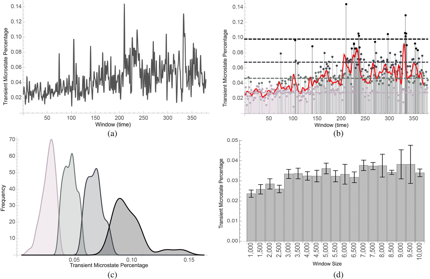
Fig. 3. (a) shows the time-varying transient microstate percentage of EEG signals (cf. the section “Physiologically-based segmentation using transient microstates and PSD”) of a subject who was asked to perform a set of tasks over 30 min. In (b), the transient microstate percentage curve was classified into low segment (lighter gray) medium segments (light gray), high segments (gray), and very high segments (black). A trending curve was added. In (c), histograms were computed. Lower microstate percentages correlated with easier tasks while higher microstate percentages correlated with harder tasks. In (d), the transient microstate percentage was computed on a subject with eyes closed using different window sizes. The percentage shows stability with respect to the window size. Distributions corresponded to segments that were computed to be easy, medium, hard, and very hard
Preliminary assessment
Our design protocols consisted of video sequences of subjects performing different design tasks of varying difficulty while having their EEG monitored. Although the number of subjects in our experiments was low (eight subjects), each design episode was long (up to 2 h of EEG data gathered per episode). After each task, the subject was asked to grade the level of difficulty of the task. The design protocol was encoded using design moves (Kan & Gero, Reference Kan and Gero2008). For example, 47 such design moves were identified in a design protocol that lasted about 30 min. Table 1 displays the first few segments of the design protocol we used.
Table 1. Segmentation of the design protocol video into design moves. Grayed-out rows were detected by means of the automated physiological method. Non-grayed-out rows were expected design moves in the segmentation that were not detected by the method
In the first set of experiments, we computed the transient percentage curve of the full design episode. The dataset used in Figure 3a is the same as the dataset used in Figure 3b. It was obtained by measuring the EEG of a subject who was asked to perform various tasks for a duration of about 30–120 min. The epochs were then divided into windows of 2500 samples at a sample rate of 500 samples per second. The transient microstate percentage of each window of about 2.5 s was computed. Figure 3a displays the transient microstate percentage curve of the full episode of the design protocol data.
In the second set of experiments, we clustered the values based on the evoked transient percentage levels of the segments. Figure 3b displays how the percentage curve was then clustered into four clusters corresponding to low, medium, high and very high effort segments. Figure 3c shows the frequency distribution of the four clusters that were discovered. Peaks in the transient microstate percentage occur at 0.03, 0.05, 0.07, and 0.09.
It can also be noted that the transient microstate percentage is a stable metric. To test this, we have computed it on subsegments of a larger segment where a subject was asked to rest. Since the larger segment was from a single design move type (resting state), it was expected that the transient microstate percentage remain stable. Such transient microstate percentages were shown to camp between 2% and 4%. Figure 3d illustrates this.
Our method performed well in the discovery of segments such as “subject thinks about a solution” or “subject consults experiment solutions”. EEGs excel at measuring states of mind. These segments are usually implicit in a design protocol and can only be detected by inspecting a video for longer than usual pauses or using concurrent verbalization techniques (assuming the thought process is reportable). However, some segments that would have been expected failed to be discovered by this method. In some cases, the method completely failed to discover transitions from non-rest to rest. This is surprising since they are the easier ones to discover using such methods. One such omission occurs at the end of the design episode and can be understood as the long-range sensitivity of the transient microstate percentage. Overall fatigue impacts the metric. On categories of design moves such as “designs”, “reads”, and “rates” and soft design moves, our method based on transient microstate percentages, performed well on average. A complete segmentation of a design protocol video is shown in Figure 4. A histogram displaying the transient microstate percentage curve is shown in the margin of the figure. The design protocol segmentation is annotated with corresponding design moves.

Fig. 4. Coarse-grained segmentation of design protocol video based on the transient microstate percentage. A window size of 5 (25 s) was chosen. Values in the window were averaged. The resulting values were clustered into four clusters
Comparisons between techniques
Experimental protocol
To evaluate the correctness and precision of EEG-based segmentation, we adopted the following strategy. First, three domain experts were asked to segment the 8 videos manually. Second, a set of nine algorithms using two different window parameters (for a total of 18 algorithms) was used to segment the videos.
In addition to the segmentation we proposed using transient microstates, we used PSD, which are commonly used in EEG analysis. A summary of those PSD algorithms is provided in Table 3. We then compared the distance between different manual segmentations by domain experts, between manual segmentation and EEG-based segmentation and between different EEG-based segmentations. This was to evaluate which algorithm performed best in comparison with manual segmentation. Also, it was expected that manual segmentation would perform the best (since comparing manual segmentations with themselves is tautological). But it was unknown to what extent. Furthermore, the relationship between different algorithms was also an unknown.
When comparing manual segmentations to manual segmentations, we evaluated if manual segmentation is self-consistent. When comparing automated segmentations with manual segmentations, we actually evaluated to what extent automated segmentation is aligned with manual segmentation. Finally, when comparing automated segmentations with automated segmentations, we evaluated if automated segmentation sees something that manual segmentation does not. If automated segmentation is self-consistent while yielding other results than manual segmentations, this may hint at an underlying structure that manual segmentations cannot see. EEG brain patterns would then be able to identify cognitive structures that simple observation cannot. The notion of perfect segmentation is ill-defined. It may not truly exist. We attempt to relativize our analysis and determine if each method is consistent and to what extent they are similar.
The distance metric we used to evaluate the deviation between two segmentations was the following nearest neighbor measure (rather than other IRR or IRA metrics such as Cohen's Kappa or intraclass correlation coefficients):
 $$d(x\comma \,y) = \sum\limits_{\rm i} {Abs(y_{\rm i} - Nearest(x\comma \,y_{\rm i}))} $$
where x and y are different segmentations (list of time stamps). The Nearest function computes the nearest neighbor of a time stamp in a segmentation compared with another segmentation. This distance measure allows for segmentations of variable lengths. However, it is a non-metric distance measure. To alleviate this, we only need to set x to be the longest or shortest segment and y to be the other remaining segmentation. Also, false and near positives are a necessary evil. False positives occur when an algorithm finds a segment that does not make sense. Near positives occur when a segment is slightly different from what was expected. If a segment has length 100 and the other 200, then it is clear that at least 100 points are false positives or near positives. This being said, false and near positives may be indicative that a segmentation contains more information than another. The labels we used for each datasets in Figures 5–7 are listed in Table 2.

Fig. 5. Standard error matrix associated with the distance matrix. See Table 2 for label descriptions
Fig. 6. Distance matrix of each of the eight datasets (from top to bottom: FEB28, FEB18, AUG5, APR18, APR16, APR8, APR23, APR21) with respect to the distance between the domain expert segmentation (R1, R2, R3). See Table 2 for label descriptions
Fig. 7. Distance matrix between various segmentation strategies averaged across the eight datasets. Distances are measured in minutes (e.g. 0.01 is equivalent to 1 s). The first three rows show the distance between Domain Expert segmentation (R1, R2, R3), and algorithm segmentation (TM1%, A1, B1, … , H2). Our nearest neighbor metric was used to compute deviations in seconds between different segmentations using different segmentation algorithms. See Table 2 for label descriptions
Table 2. Segment labels and methods for different window parameters
PSD were measured on the FP1 electrode of the EEG as commonly performed. The transient microstates were computed on all 64 electrodes of the EEG device. Table 3 shows the characteristics of the different PSD algorithms we chose.
Table 3. EEG frequency-domain features
Figure 7 shows the distance matrix of the 21 segmentations obtained (three domain expert segmentations, nine EEG-based segmentations with window size parameter set to 1 and 9 EEG-based segmentations with window size parameter set to 2). Each distance in the distance matrix was averaged from the segmentations obtained for each of the eight datasets (FEB28, FEB18, AUG5, APR18, APR16, APR8, APR23, APR21). Figure 5 shows the standard errors associated with the distance matrix resulting from the averaging process. Figure 6 shows the unaveraged results for the first three rows of the distance matrix corresponding to the distance between domain expert segmentation and EEG-based segmentation.
Statistical significance using z-tests was done against the hypothesis that the mean of the average difference was equal to 1 s. For domain expert R2, the only domain expert segmentation to deviate from the 1 s mean, p-value was found to be 0.3467 which lead to failure to reject the null hypothesis. This means that differences between average deviations for domain expert are not statistically significant. For the best scoring algorithm (TM1%), the average distance was found to be 2 s. It had p-value 0.002129 which lead to rejection of the null hypothesis. Differences between domain expert segmentation and algorithm segmentation were then found to be statistically significant. Furthermore, we computed Cohen's D to get an idea of the effect size of our results in Table 4. Note that TM1%, our best performing algorithm in terms of deviation from domain expert segmentation, has a 0.64 D-score when compared with the deviation between R1 and R2. This shows a medium effect size indicating that algorithm TM1% was averagely indistinguishable from the deviation between domain experts R1 and R2. All other D-scores were large. Domain expert and algorithm segmentation were generally distinguishable from each other, which supports our statistical significance tests (z-test). Algorithmic segmentation based on transient microstate percentages is not a replacement for domain expert segmentation. It provides another glimpse at cognitive processes and approximates manual segmentation. Manual segmentation is based on the designer's visible behavior, which may not always reflect the designer's inner thought process.
Table 4. Effect size using Cohen's D for the average deviation of different algorithms compared with the deviation between domain experts R1–R2, R1–R3, and R2–R3. The best performing algorithm is shown in bold. Smaller D-scores are better because they indicate less variation between the raters (note that the usual interpretation of D-scores is “bigger is better”)
Domain expert versus domain expert
Domain expert segmentation is a lengthy task especially on long video protocols like the ones we gathered. This alone is motivation for automated techniques. As expected, the deviation is lowest for domain expert to domain expert comparisons (the first three columns). The average distance of the first domain expert segmentation to the two others was 1 s, the average distance of the second domain expert segmentation to the two others was 1.3 s and the average distance of the third domain expert segmentation was 1 s. In this experimental context, it was expected that domain expert segmentation performed the best. While subjectivity of segmentation (deciding if a given segment-event in the videos is worth notice) was a factor, the metric we used alleviated false and near positives. Therefore, a 1–1.3 s deviation between different domain expert segmentations is expected and realistic. All domain experts were presented the same videos. Their reactions to the videos were, therefore, expected to be similar.
Domain-expert-to-domain-expert comparisons serve mostly the purpose of being a benchmark value: a 1–1.3 s average deviation in segments is, therefore, expected to be a normal and natural deviation.
Algorithm versus domain expert
The best EEG-based segmentation had a 2 s deviation and was obtained by the transient microstate algorithm with window parameter set to 1. The worst result was a 12 s deviation and was obtained by the beta PSD algorithm with window parameter set to 2. In the case of the best result, we determined that a 1 s difference between the average distance of domain expert and EEG-based segmentations entailed that both segmentation methods were good. Microstate-based segmentation (the best performing algorithm) is a holistic measure on all 64 electrodes of an EEG. Any movement in the EEG is recorded and accounted for in the microstate algorithm. The power spectral density algorithms did not perform as well. Using a window size of 1, they averaged a difference ranging from 2.3 s in the best case (theta/beta formula) to 8.3 s (theta formula) for an average of 5.3 s on algorithms. Using a window size of 2, they ranged from 7.7 (alpha/beta formula) seconds to 12 s (beta formula) for an average of 9.7 s on algorithms. It can be noticed that larger window sizes may have caused larger differences but also incur less false and near positives.
The higher differences recorded on PSD algorithms can be explained. As Table 3 shows, the PSD formulas used measure relaxation, focus, concentration, attention, and fatigue. These characteristics are not easily visible in a video recording of a subject solving design tasks. Indeed, do concentration or fatigue translate automatically into a pause in the video recording? Therefore, although average differences were higher with PSD-based algorithms, this does not mean that PSD-based algorithms provide erroneous segmentations. They rather provide complementary information on the design videos, more specifically, information that is not easily seen in the recordings.
Brain activities do not always align with their outward behavior. Therefore, benchmarking EEG segmentation with domain expert manual segmentation may not be always significant.
Figure 8 compares manual segmentation by a domain expert and automated segmentation using the transient microstate algorithm by aligning screenshots from the experimental protocol with found segments.
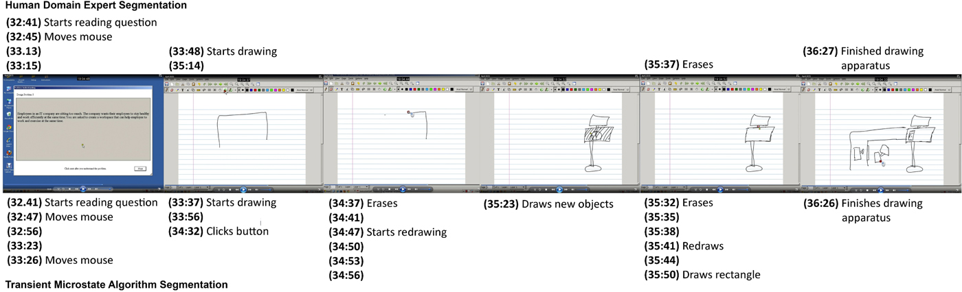
Fig. 8. Sequence of screenshots from experimental protocol comparing manual segmentation and automated segmentations: (top) lists segments found by a domain expert; (bottom) shows segments found by the transient microstate algorithm with window size 1. Major segments (screenshot 1, 2, 5, and 6) are roughly aligned when comparing domain expert segmentation and automated segmentation. Automated segmentation is however much more fine-grained than manual segmentation. Unlabeled segments show segments that are observed to be a continuation of the previous segment label and for which no obvious observation can be made
Algorithm versus algorithm
By inspecting Figure 7, we notice that the average deviation between domain expert segmentation and algorithms is higher than deviation between different algorithms. This seems to point to a certain consistency between algorithms. Therefore, the first three rows and columns are labeled using a darker color as we move outwards while the submatrix, composed of the other columns, remains relatively within low values. By inspecting Figure 7, we also notice that on some datasets, some algorithms performed better than the best average algorithm (transient microstates), even yielding 0-deviation values. Also, on average, EEG-based segmentations using a window size of 1 performed better than those using a window size of 2. This is partly because lower window size values generate larger segmentations and therefore cause more false positives or near positives. False positives occur when an irrelevant segment is found whereas near positives occur when almost relevant segments are found. However, as expected, domain expert segmentations are more similar to each other. The transient microstate algorithm with window size 1 performs the best as it incorporates data from all the 64 electrodes of the EEG apparatus.
Different EEG-based segmentations seem to correlate with each other. This may hint at the fact that while the hardness of a design task increases, stress, fatigue or concentration may increase or decrease as well in a correlated manner. More specifically, the transient microstate algorithm (row 4 of Fig. 7) seemed to remain in the range of 1–3 s deviation over all datasets while most other PSD-based algorithms seemed to remain in the range of 1–6 s when compared with each other with occasional spikes in the 7–9 s range.
Comparing domain expert segmentation to algorithm-based segmentation provides insight into how well an algorithm aligns with the intuition of what a segmentation should be. Comparing algorithms to each other provides additional information based on the characteristics that each algorithm measures.
Figure 9 compares two automated segmentation algorithms by aligning screenshots from the experimental protocol with found segments.

Fig. 9. Sequence of screenshots from experimental protocol comparing two automated segmentations: (top) lists segments found by the transient microstate algorithm with window size 1; (bottom) shows segments found by the beta algorithm with window size 1. The beta algorithm misses a few segments and shows a slight deviation from the transient microstate algorithm. However, in screenshot 6, the beta algorithm showed a high level of granularity for the “Stops and thinks” segment. This can be explained by the fact that the beta range measures concentration
Conclusion
We have outlined the application of a physiological method to perform design protocol analysis based on EEG and microstate analysis. Current techniques for design protocol segmentation involve a manual step of encoding the protocol. A particular choice of encoding captures the richness of information contained in design protocols. It can be noted that the transition from textual to non-textual sources entails both a loss of information and a gain of information. We have taken the approach of solving the problem using a fully automated tool. We discussed the implications of this. Physiological techniques are ubiquitous to design research and we have proposed a method of segmenting design protocols into logical units using EEG. Based on a series of experimental validations, the method performed well on average and was able to discover the time dimension of different design moves adequately with respect to a manual segmentation process. The transient microstate algorithm performed better than PSD-based algorithms and compared well with segmentation by domain experts. EEG-based segmentation of design protocols is a feasible approach to protocol segmentation.
Acknowledgments
We wish to thank NSERC for the Discovery Grant that has supported this research. We also wish to thank the volunteers from the Faculty of Engineering and Computer Sciences for their participation in our experiments.
Philon Nguyen received his PhD degree at the Concordia Institute for Information Systems Engineering in April 2017 in Montreal, Canada. He received his Bachelor's and Master's degree in Computer Science, both from Concordia University, respectively, in 2007 and 2009. His research interests include design cognition and design theories and methodologies, machine learning and data mining.
Thanh An Nguyen received her PhD degree in August 2016 from the Electrical and Computer Engineering Department at Concordia University, Montreal, Canada. She received her Bachelor's degree in Computer Science and Master's degree in Information System Security, both from Concordia University respectively in 2006 and 2009. Her research interests include design cognition, human visual perception, and curve reconstruction. She can be reached at thanhan.nguyen@mail.concordia.ca.
Yong Zeng is a Professor in the Concordia Institute for Information Systems Engineering at Concordia University. He is NSERC Chair in Aerospace Design Engineering (July 2015–June 2020) and was the Canada Research Chair (Tier II) in design science (April 2004–August 2014). He received a PhD (Mechanical and Manufacturing Engineering) in 2001 at the University of Calgary and another PhD (Computational Mechanics) in 1992 at Dalian University of Technology. His research aims to understand and improve creative design activities, which crosses design, computer science, mathematics, linguistics, and neurocognitive science. He has proposed the Environment-Based Design (EBD) theory.


