


1. INTRODUCTION
Current methods of designing and optimizing antennas by hand are time and labor intensive, limit complexity, and require significant expertise and experience. Evolutionary design techniques can overcome these limitations by searching the design space and automatically finding effective solutions that would ordinarily not be found. Researchers have been investigating evolutionary antenna design and optimization since the early 1990s (e.g., Michielssen et al., Reference Michielssen, Sajer, Ranjithan and Mittra1993; Haupt, Reference Haupt1995; Altshuler & Linden, 1997b; Rahmat & Michielssen, 1999), and the field has grown in recent years as computer speed has increased and electromagnetics simulators have improved. Many antenna types have been investigated, including wire antennas (Linden & Altshuler, Reference Linden and Altshuler1996), antenna arrays (Haupt, Reference Haupt1996), and quadrifilar helical (QFH) antennas (Lohn et al., Reference Lohn, Kraus and Linden2002). In addition, the ability to evolve antennas in situ (Linden, Reference Linden2000), that is, taking into account the effects of surrounding structures, opens new design possibilities. Such an approach is very difficult for antenna designers because of the complexity of electromagnetic interactions, yet easy to integrate into evolutionary techniques. Below we describe two evolutionary algorithm (EA) approaches to a challenging antenna design problem on NASA's Space Technology 5 (ST5) mission.Footnote 1 ST5's objective is to demonstrate and flight-qualify innovative technologies and concepts for application to future space missions. An image showing the ST5 spacecraft is seen in Figure 1.
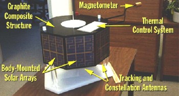
Fig. 1. ST5 satellite mockup. The satellite has two antennas, centered on the top and bottom of each spacecraft. [A color version of this figure can be viewed online at journals.cambridge.org/aie]
2. ST5 MISSION ANTENNA REQUIREMENTS
The three ST5 spacecraft will orbit at close separations in a highly elliptical geosynchronous transfer orbit approximately 35,000 km above Earth, and will communicate with a 34-m ground-based dish antenna. The combination of wide beamwidth for a circularly polarized wave and wide bandwidth make for a challenging design problem. In terms of simulation challenges, because the diameter of the spacecraft is 54.2 cm, the spacecraft is approximately 14 wavelengths across, which makes antenna simulation computationally intensive. For that reason, an infinite ground plane approximation or smaller finite ground plane is typically used in modeling and design.
The antenna requirements are as follows. The gain pattern must be greater than or equal to 0 dBic (decibels as referenced to an isotropic radiator that is circularly polarized) at 40° ≤ θ ≤ 80° and 0° ≤ φ ≤ 360° for right-hand circular polarization. The antenna must have a voltage standing wave ratio (VSWR) of under 1.2 at the transmit frequency (8470 MHz) and under 1.5 at the receive frequency (7209.125 MHz): VSWR is a way to quantify reflected-wave interference, and thus the amount of impedance mismatch at the junction. At both frequencies the input impedance should be 50 Ω. The antenna is restricted in shape to a mass of under 165 g, and must fit in a cylinder of height and diameter of 15.24 cm.
In addition to these requirements, an additional “desired” specification was issued for the field pattern. Because of the spacecraft's relative orientation to the Earth, high gain in the field pattern was desired at low elevation angles. Specifically, across 0° ≤ φ ≤ 360°, gain was desired to meet: 2 dBic for θ = 80°, and 4 dBic for θ = 90°.
ST5 mission managers were willing to accept antenna performance that aligned closer to the “desired” field pattern specifications noted above, and the contractor, using conventional design practices, produced a QFH (see Fig. 2) antenna to meet these specifications.
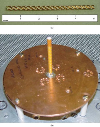
Fig. 2. Conventionally designed QHF antenna: (a) radiator (scale in inches) and (b) radiator mounted on a ground plane. [A color version of this figure can be viewed online at journals.cambridge.org/aie]
3. EVOLVED ANTENNA DESIGN
From past experience in designing wire antennas (Linden, Reference Linden1997), we decided to constrain our evolutionary design to a monopole wire antenna with four identical arms, each arm rotated 90° from its neighbors. The EA thus evolves genotypes that specify the design for one arm, and builds the complete antenna using four copies of the evolved arm. In the remainder of this section we describe the two evolutionary algorithms used. The first algorithm was used in our previous work in evolutionary antenna design (Linden & Altshuler, Reference Linden and Altshuler1996), and it is a standard genetic algorithm (GA) that evolves nonbranching wire forms. The second algorithm is based on our previous work evolving rod-structured, robot morphologies (Hornby & Pollack, Reference Hornby and Pollack2002). This EA has a genetic programming (GP) style tree-structured representation that allows branching in the wire forms. In addition, the two EAs use different fitness functions.
3.1. Parameterized EA
In this EA, the design was constrained to nonbranching arms and the encoding used real numbers. The feed wire for the antenna is not optimized, but is specified by the user. The size constraints used, an example of an evolved arm, and the resulting antenna are shown in Figure 3.
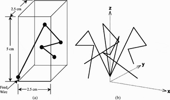
Fig. 3. (a) Size constraints and evolved arm and (b) the resulting four-wire antenna after rotations.
3.1.1. Representation
The design is specified by a set of real-valued scalars, one for each coordinate of each point. Thus, for a four-segment design (shown in Fig. 3), 12 parameters are required. Adewuya's method of mating (Adewuya, Reference Adewuya1996) and Gaussian mutation are used to evolve effective designs from initial random populations. This EA has been shown to work extremely well on many different antenna problems (Altshuler & Linden, 1997; Altshuler, Reference Altshuler2002; Linden, Reference Linden2000).
3.1.2. Fitness function
This EA used pattern quality scores at 7.2 and 8.47 GHz in the fitness function. Unlike the second EA, VSWR was not used in this fitness calculation. To quantify the pattern quality at a single frequency, PQf, the following was used:

where gainφ,θ is the gain of the antenna (dBic, right-hand polarization) at a particular angle, T is the target gain (3 dBic was used in this case), φ is the azimuth, and θ is the elevation. To compute the overall fitness of an antenna design, the pattern quality measures at the transmit and receive frequencies were summed, lower values corresponding to better antennas:
3.2. Open-ended EA
The EA in this section allows for branching in the antenna arms. Rather than using linear sequences of bits or real values as is traditionally done, here we use a tree-structured representation that naturally represents branching in the antenna arms.
3.2.1. Representation
The open-ended representation for encoding branching antennas is an extension of our previous work in using a linear representation for encoding rod-based robots (Hornby & Pollack, Reference Hornby and Pollack2002). Each node in the tree-structured representation is an antenna-construction command, and an antenna is created by executing the commands at each node in the tree, starting with the root node. In constructing an antenna the current state (location and orientation) is maintained and commands add wires or change the current state. The commands are as follows:
•
forward(length,radius): add a wire with the given length and radius extending from the current location and then change the current state location to the end of the new wire.•
rotate-x(angle): change the orientation by rotating it by the specified amount (in radians) about the x-axis.•
rotate-y(angle): change the orientation by rotating it by the specified amount (in radians) about the y-axis.•
rotate-z(angle): change the orientation by rotating it by the specified amount (in radians) about the z axis.
An antenna design is created by starting with an initial feedwire and adding wires. For the ST5 mission the initial feed wire starts at the origin and has a length of 0.4 cm along the z axis. That is, the design starts with the single feedwire from (0.0, 0.0, 0.0) to (0.0, 0.0, 0.4) and the current construction state (location and orientation) for the next wire will be started from location (0.0, 0.0, 0.4) with the orientation along the positive z axis. To produce antennas that are four-way symmetric about the z axis, the construction process is restricted to producing antenna wires that are fully contained in the positive XY quadrant, and then after construction is complete, this arm is copied three times and these copies are placed in each of the other quadrants through rotations of 90°, 180°, and 270°. For example, in executing the program
, the
command causes the current orientation to rotate 0.523598776 radians (30°) about the Z axis. The
command adds a wire of length 1.0 cm and radius 0.032 cm in the current forward direction. This wire is then copied into each of the other three XY quadrants. The resulting antenna is shown in Figure 4a.

Fig. 4. Example antennas: (a) nonbranching arms and (b) branching arms.
Branches in the representation cause a branch in the flow of execution and create different branches in the constructed antenna. The following is an encoding of an antenna with branching in the arms, here brackets are used to separate the subtrees:
This antenna is shown in Figure 4b.
To take into account imprecision in manufacturing an antenna, antenna designs are evaluated multiple times, each time with a small random perturbation applied to joint angles and wire radii. The overall fitness of an antenna is the worst score of these evaluations. In this way, the fitness score assigned to an antenna design is a conservative estimate of how well it will perform if it were to be constructed. An additional side effect of this is that antennas evolved with this manufacturing noise tend to perform well across a broader range of frequencies than do antennas evolved without this noise.
3.2.2. Fitness function
The fitness function used to evaluate antennas is a function of the VSWR and gain values on the transmit and receive frequencies. The VSWR component of the fitness function is constructed to put strong pressure to evolving antennas with receive and transmit VSWR values below the required amounts of 1.2 and 1.5, reduced pressure at a value below these requirements (1.15 and 1.25), and then no pressure to go below 1.1:

where v r is the VSWR at the receive frequency, v t is the VSWR at the transmit frequency, and VSWR = v r′v t′.
The gain component of the fitness function uses the gain (decibels) in 5° increments about the angles of interest from 40° ≤ θ ≤ 90° and 0° ≤ φ ≤ 360°:

Although the actual minimum required gain value is 0 dBic for 40° ≤ θ ≤ 80°, and desired gain values are 2 dBic for θ ≥ 80° and 4 dBic for θ = 90°, only a single target gain of 0.5 dBic is used here. This provides some headroom to account for errors in simulation over the minimum of 0 dBic and does not attempt to meet desired gain values. Because achieving gain values greater than 0 dBic is the main part of the required specifications, the third component of the fitness function reward antenna designs for having sample points with gains greater than zero:

These three components are multiplied together to produce the overall fitness score of an antenna design:
The objective of the EA is to produce antenna designs that minimize F.
4. EA RUN SETUP
An 80-node Linux cluster was used to run the open-ended EA. The nodes were composed of AMD Athlon CPUs running at speeds between 1.4 and 2.1 GHz. Each CPU has access to 500 MB of memory and each node runs diskless. Standard office Ethernet connects the CPUs.
As mentioned earlier, the ST5 spacecraft is 13–15 wavelengths wide, which makes simulation of the antenna on the full craft very compute intensive. To keep the antenna evaluations fast, an infinite ground plane approximation was used in all runs. This was found to provide sufficient accuracy to achieve several good designs. Designs were then analyzed on a finite ground plane of the same shape and size as the top of the ST5 body to determine their effectiveness at meeting requirements in a realistic environment. The Numerical Electromagnetics Code, Version 4 (NEC4; Burke, 1981) was used to evaluate all antenna designs.
For the parameterized EA, a population of 50 individuals was used, 50% of which is kept from generation to generation. The mutation rate was 1%, with the Gaussian mutation standard deviation of 10% of the value range. The parameterized EA was halted after 100 generations had been completed, the EA's best score was stagnant for 40 generations, or EA's average score was stagnant for 10 generations. For the open-ended EA, a population of 200 individuals was created through either mutation or recombination, with an equal probability. For both algorithms, each antenna simulation took a few seconds of wall-clock time to run, and an entire run took approximately 6 –10 h on 35 nodes of the cluster described above. In summary, Table 1 summarizes the key features of the problem of synthesizing an ST5 antenna in the context of the open-ended EA.
Table 1. ST5 X-band antenna, open-ended evolutionary algorithm

VSWR, voltage standing wave ratio.
Antenna designs are initially created randomly, and hence many initial designs are unsimulatable and cause NEC4 to abort. When we create the initial generation (gen 0) we only place simulatable antenna designs into the population. Although a noticeable percentage of designs fail to simulate in the initial generations, this drops to near zero as evolution proceeds.
5. EVOLVED ANTENNA RESULTS
The two best evolved antennas, one from each of the EAs described above, were fabricated and tested. The antenna named ST5-3-10 was produced by the open-ended EA that allowed branching, and the antenna named ST5-4W-03 was produced by the other EA. Photographs of the prototyped antennas are shown in Figure 5. Because of space limitations, only performance data from antenna ST5-3-10 is presented below.
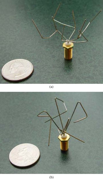
Fig. 5. Photographs of prototype evolved antennas: (a) ST5-3-10 and (b) ST5-4W-03. [A color version of this figure can be viewed online at journals.cambridge.org/aie]
Because the goal of our work was to produce requirements-compliant antennas for ST5, no attempt was made to compare the algorithms, either to each other, or to other search techniques. Thus statistical sampling across multiple runs was not performed.
Evolved antenna ST5-3-10 is 100% compliant with the mission antenna performance requirements. This was confirmed by testing the prototype antenna in an anechoic test chamber at NASA Goddard Space Flight Center. The data measured in the test chamber is shown in the plots below.
The genotype of antenna ST5-3-10 is given in Appendix A. The complexity of this large antenna-constructing program, compared to the antenna arm design having one branch, suggests that it is not a minimal description of the design. For example, instead of using the minimal number of rotations to specify relative angles between wires (two) there are sequences of up to a dozen rotation commands.
The 8.47-GHz maximum/minimum gain patterns for both antennas are shown in Figure 6. On the plots for antenna ST5-3-10, a box denoting the acceptable performance according to the requirements is shown. Note that the minimum gain falls off steeply below 20°. This is acceptable as those elevations were not required because of the orientation of the spacecraft with respect to Earth. As noted above, the QFH antenna was optimized at the 8.47 GHz frequency to achieve high gain in the vicinity of 75°–90°.

Fig. 6. Maximum and minimum gain at 8.47 GHz for (a) ST5-3-10 and (b) QFH antennas. [A color version of this figure can be viewed online at journals.cambridge.org/aie]
6. RESULTS ANALYSIS
Antenna ST5-3-10 is a requirements-compliant antenna that was built and tested on an antenna test range. Although it is slightly difficult to manufacture without the aid of automated wire-forming and soldering machines, it has a number of benefits as compared to the conventionally designed antenna.
First, there are potential power savings. Antenna ST5-3-10 achieves high gain (2–4 dB) across a wider range of elevation angles. This allows a broader range of angles over which maximum data throughput can be achieved and would result in less power being required from the solar array and batteries.
Second, unlike the QFH antenna, the evolved antenna does not require a matching network nor phasing circuit, removing two steps in design and fabrication of the antenna. A trivial transmission line may be used for the match on the flight antenna, but simulation results suggest that one is not required if small changes to the feedpoint are made.
Third, the evolved antenna has more uniform coverage in that it has a uniform pattern with small ripples in the elevations of greatest interest (40°–80°). This allows for reliable performance as elevation angle relative to the ground changes.
Fourth, the evolved antenna had a shorter design cycle. It was estimated that antenna ST5-3-10 took 3 person-months to design and fabricate the first prototype as compared to 5 person-months for the QFH antenna.
From an algorithmic perspective, both evolutionary algorithms produced antennas that were satisfactory to the mission planners. The branching antenna, evolved using a GP-style representation, slightly outperformed the nonbranching antenna in terms of field pattern and VSWR. A likely reason as to why the GP-style representation performed better is that it is more flexible and allows for the evolution of new topologies.
7. RE-EVOLVED ANTENNA RESULTS
In total, it took us approximately 4 weeks to both modify our two EAs and evolve new antennas for the revised mission requirements. The configuration of the two EAs (population size, selection/replacement, variation, etc.) remained the same as in the first set of evolutionary runs. Again, the best antennas evolved by the two EAs were then evaluated on a second antenna simulation package, WIPL-D, with the addition of a 6-in. ground plane to determine which designs to fabricate and test on the ST5 mock-up. Based on these simulations the best antenna design from each EA was selected for fabrication, and these are shown in Figure 7: ST5-33.142.7 was evolved using the open-ended EA (Fig. 7a) and ST5-104.33 was evolved using the parameterized EA (Fig. 7b). A sequence of evolved antennas that produced antenna ST5-33.142.7 is shown in Figure 8.
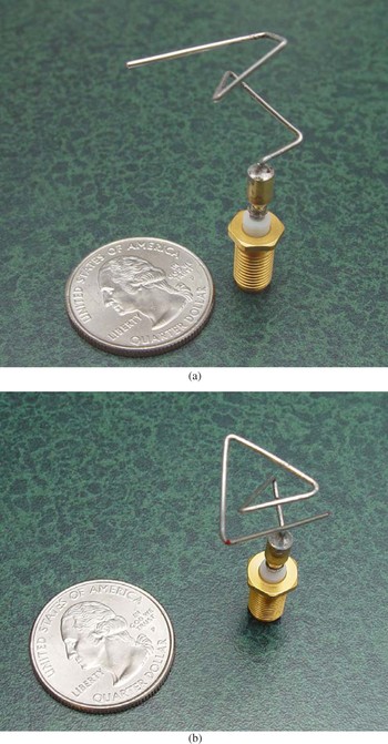
Fig. 7. Evolved antenna designs: (a) evolved using a constructive process (ST5-33.142.7) and (b) evolved using a vector of parameters (ST5-104.33). [A color version of this figure can be viewed online at journals.cambridge.org/aie]

Fig. 8. The sequence of evolved antennas leading up to antenna ST5-33.142.7. [A color version of this figure can be viewed online at journals.cambridge.org/aie]
Both ST5-33.142.7 and ST5-104.33 have excellent simulated RHCP patterns for the transmit frequency, as shown in Figure 9. The antennas also have good circular polarization purity across a wide range of angles, as shown in Figure 10 for ST5-104.33. To the best of our knowledge, this quality has never been seen before in this form of antenna.

Fig. 9. Simulated 3-dimensional patterns for (a) ST5-33.142.7 and (b) ST5-104.33 on a 6-in. ground plane at 8470 MHz for RHCP polarization. Simulation performed by WIPL-D. Patterns are similar for 7209 MHz. [A color version of this figure can be viewed online at journals.cambridge.org/aie]

Fig. 10. RHCP versus LHCP performance of ST5-104.33. The plot has 2 dB/division. [A color version of this figure can be viewed online at journals.cambridge.org/aie]
Because two antennas are used on each spacecraft, and not just one, it is important to measure the overall gain pattern with two antennas mounted on the spacecraft. For this, different combinations of the two evolved antennas and the QHA were tried on the the ST5 mockup and measured in an anechoic chamber (Fig. 11). With two QHAs, 38% efficiency was achieved, using a QHA with an evolved antenna resulted in 80% efficiency, and using two evolved antennas resulted in 93% efficiency. Figure 12 shows these measured results for the combination of two QHAs together, a QHA and an ST5-104.33 and for two evolved antennas.

Fig. 11. Photograph of the ST5 mockup with antennas mounted (only the antenna on the top deck is visible). [A color version of this figure can be viewed online at journals.cambridge.org/aie]

Fig. 12. Measured patterns on the ST-5 mockup of two QHAs and an ST5-104.33 with a QHA. Phi 1 = 0°, Phi 2 = 90°. [A color version of this figure can be viewed online at journals.cambridge.org/aie]
8. CONCLUSION
We have evolved and built X-band antennas for the initial ST5 mission requirements and for the revised ST5 mission requirements. It took approximately 4 months to set up our evolutionary algorithms and produce the first set of evolved antennas that were shown to be compliant with respect to the original ST5 antenna performance requirements. In response to an orbit change, it took roughly 4 weeks to evolve a new antenna, which was acceptable to mission managers for the revised set of mission requirements. One evolved antenna is in use on each of the three ST5 spacecraft and, with their successful launch on March 22, 2006, they have become the first computer-evolved antennas to be deployed and the first computer-evolved hardware in space.
In addition to being the first evolved hardware in space, the evolved antennas demonstrate several advantages over the conventionally designed antennas and manual design in general. The evolutionary algorithms we used were not limited to variations of previously developed antenna shapes but generated and tested thousands of completely new types of designs, many of which have unusual organic-looking structures that expert antenna designers would not be likely to produce. Compared to the conventional antenna, the evolved antenna has these benefits:
• better coverage
• significantly higher efficiency
• fewer parts: lower cost, increased reliability, easier manufacture
• naturally matched to 50 Ω
• faster design time
• rapid redesign accomplished at a small cost and in a short time frame
By exploring such a wide range of designs EAs may be able to produce designs of previously unachievable performance. For example, the best antennas we evolved achieve high gain across a wider range of elevation angles, which allows a broader range of angles over which maximum data throughput can be achieved and may require less power. In addition, our flight antenna has a very uniform pattern with small ripples in the elevations of greatest interest (40–80°), which allows for reliable performance as elevation angle relative to the ground changes. With the evolutionary design approach it took approximately 3 person-months of work to generate the initial evolved antennas versus 5 person-months for the conventionally designed antenna, and when the mission orbit changed, with the evolutionary approach we were able to modify our algorithms and re-evolve new antennas specifically designed for the new orbit and prototype hardware in 4 weeks. The faster design cycles of an evolutionary approach results in less development costs and allows for an iterative “what-if” design and test approach for different scenarios. This ability to rapidly respond to changing requirements is of great use to NASA because NASA mission requirements frequently change. As computer hardware becomes increasingly more powerful and as computer modeling packages become better at simulating different design domains we expect evolutionary design systems to become more useful in a wider range of design problems and gain wider acceptance and industrial usage.
ACKNOWLEDGMENTS
The work described in this paper was supported by Mission and Science Measurement Technology, NASA Headquarters, under its Computing, Information, and Communications Technology Program. Research was performed at the Computational Sciences Division, NASA Ames Research Center, Linden Innovation Research, and NASA Goddard Space Flight Center. The support of Ken Perko of Microwave Systems Branch at NASA Goddard and Bruce Blevins of the Physical Science Laboratory at New Mexico State University is gratefully acknowledged.
Jason D. Lohn is a Senior Research Scientist at Carnegie Mellon University. He has worked at Google, NASA Ames Research Center, Stanford University, and IBM. He received an MS and a PhD in electrical engineering from the University of Maryland at College Park. He led research in evolvable systems while at NASA and did early work in the field of evolvable hardware. He cofounded a series of successful NASA/DoD evolvable hardware conferences. Dr. Lohn is a member of IEEE, ACM, and Sigma Xi. He has over 50 technical publications and serves as an Associate Editor of IEEE Transactions on Evolutionary Computation.
Greg Hornby was a Visiting Researcher at Sony's Digital Creatures Laboratory from 1998 to 1999 and is currently a senior scientist with University of California Santa Cruz at NASA Ames Research Center. He received his PhD in computer science from Brandeis University in 2002. His interests cover computer-automated design, generative representations, and complexity measures. In addition to creating the EA that evolved the ST-5 spacecraft, Dr. Hornby created the EA that autonomously evolved the dynamic gait used on Sony's AIBO robot and developed the Age-Layered Population Structure EA for reducing the problem of premature convergence.
Derek Linden graduated from the USAF Academy (BS 1991) and MIT (MS 1993, PhD 1997). He has performed ground-breaking research in the automated design of wire and patch antennas using evolutionary optimization since 1995 and is coinventor of the patented genetic antenna design process. Dr. Linden has a publication list that includes 2 conference keynote addresses; 30 conference, journal, and magazine articles; 35 conference presentations (8 invited); 5 book chapters; and 2 IEEE short courses. His award-winning genetic antenna work has been highlighted in many publications, including The New York Times, Wired, Technology Review, Aviation Week, and Popular Science.
APPENDIX A
Listed below is the evolved genotype of antenna ST5-3-10. The format for this tree-structured genotype consists of the operator followed by a number stating how many children this operator has, followed by square brackets which start “[”and end “]” the list of the node's children. For example, the format for a node that is Operator 1 and has two subtrees is written
. The different operators in the antenna-constructing language are given in Section 3.2.


