Introduction
The aerospace community has introduced a system engineering concept called digital twin, which refers to an exact mirror image of a real-life aspect (e.g., flying of a spacecraft) in the cyberspace using the multi-scale, multi-physics, and probabilistic simulation that is aided by the sensor updates and historical data (Glaessgen and Stargel, Reference Glaessgen and Stargel2012). This has inspired the research community of the futuristic manufacturing systems (e.g., Industry 4.0, smart manufacturing, and connected factory). As such, the digital twins of manufacturing aspects are expected to populate the systems (e.g., cyber-physical systems) that are needed for functionalizing the futuristic manufacturing systems (Grieves and Vickers, Reference Grieves and Vickers2017; Ullah, Reference Ullah2019). The research on digital twin construction reports its myriad interplays with various aspects of futuristic manufacturing systems. Some of the recent articles are described below.
Rosen et al. (Reference Rosen, Wichert, Lo and Bettenhausen2015) described the role of digital twin for converting a manufacturing system from an automated system (sensor-actuator-execution) to an autonomous system by adding knowledge and skill bases to the sensor-actuator-execution module. Alam and Saddik (Reference Alam and Saddik2017) proposed the architecture of the digital twins for functionalizing the cyber-physical systems where the key elements are physical things, digital twins of the physical things, complex things comprising of the hierarchically structured subsystems, relationship networks among the complex things, and integration nodes of the web services. Kritzinger et al. (Reference Kritzinger, Karner, Traar, Henjes and Sihn2018) reviewed the research on the digital twin used in manufacturing, and showed that the usages of sensor signals, shape information, data formatting (RIDF, XML, AutomationML, and alike), semantic web technology, and simulation technology either for constructing the digital twins or for functionalizing it within the framework of futuristic manufacturing systems. Schroeder et al. (Reference Schroeder, Steinmetz, Pereira and Espindola2016) have outlined the IT infrastructure for constructing a manufacturing digital twin using AutomationML. Uhlemann et al. (Reference Uhlemann, Schock, Lehmann, Freiberger and Steinhilper2017) described that there are three types of digital twins, namely, digital shadow (real-time data links), digital twin for data manipulation, and digital twin for process parameter optimization, which must work in a systematic manner for reducing lead time due to the data acquisition in manufacturing systems. Qi et al. (Reference Qi, Tao, Zuo and Zhao2018) provided a broader picture of digital twin by elucidating its existence at the three levels of systemization, namely, job-shop level, manufacturing system level, and manufacturing system-of-system level. Haag and Anderl (Reference Haag and Anderl2018) described the concept of digital twin using the case of a bending beam test bench to incorporate it into the next generation manufacturing systems. Talkhestani et al. (Reference Talkhestani, Jazdi, Schloegl and Weyrich2018) showed that there must be some universal resources called anchor points that contain the detailed information regarding the machine tools, software packages, and electric devices for checking the consistency of the digital twins meant for the job-shop environment. Scaglioni and Ferretti (Reference Scaglioni and Ferretti2018) developed the digital twins of a serial machine tool structure using the FEM and of a material removal process using the kinematic analysis. The twins can be used to regulate the chatter vibration in milling. Schleich et al. (Reference Schleich, Anwer, Mathieu and Wartzack2017) described the concept of a digital twin from the perspective of the shape of an object. Botkina et al. (Reference Botkina, Hedlind, Olsson, Henser and Lundholm2018) developed the digital twin of a cutting tool by organizing the information of the components of a cutting tool using the international standard (ISO 13399), which is needed to functionalize the IoT devices for optimizing a machining operation. They also described that the digital twins provide the contents necessary for performing, coordinating, and optimizing manufacturing activities. Lu and Xu (Reference Lu and Xu2018) developed the semantic model of CNC machine tool using concept maps (Ullah et al., Reference Ullah, Arai and Watanabe2013) (a personalized ontological network) that can be used to construct the digital twins of the manufacturing resources. Luo et al. (Reference Luo, Hu, Zhu and Tao2018) proposed the concept of digital twin for making the CNC machine tool more intelligent where the knowledge acquisition and management modules are integrated with the control mechanism of the machine tool. Hu et al. (Reference Hu, Nguyen, Tao, Leu, Liu, Shahriar and Sunny2018) showed how to connect different types of physical and virtual agents using MTConnect Protocol for creating the digital twin-based manufacturing systems. Kunath and Winkler (Reference Kunath and Winkler2018) reported that digital twin emerged from the development of simulation technology. They proposed a framework of digital twin where the data and information systems are integrated with both physical and virtual manufacturing systems (e.g., manufacturing equipment systems, material flow systems, value stream system, operating material system, and human resource system). Padovano et al. (Reference Padovano, Longo, Nicoletti and Mirabelli2018) showed how to convert an existing manufacturing environment to a manufacturing environment that is in line with the concept of futuristic manufacturing systems using digital twins where the twins encapsulate and transfer knowledge required within the cyber-physical systems. They also showed an architecture to integrate the digital twins. Söderberg et al. (Reference Söderberg, Wärmefjord, Carlson and Lindkvist2017) described the digital twins for a sheet metal assembly line. They showed that for ensuring desired geometry of a sheet metal product, the geometric representation of the assembly, kinematic relations, FEA functionality, Monte Carlo simulation, material properties, and the links to the inspection databases must be integrated. Olivotti et al. (Reference Olivotti, Dreyer, Lebek and Breitner2018) proposed a concept called installed base (detailed knowledge of machines, components, and subcomponents associated with a manufacturing facility), which should be combined with the sensor data for building the digital twins of manufacturing services. Zhuang et al. (Reference Zhuang, Liu and Xiong2018) described the role of the digital twin of an assembly shop floor as the core component of a cyber-physical system. The digital twins must be integrated with real-time data acquisition systems and the historical data in the form of big-data. Tao et al. (Reference Tao, Cheng, Qi, Zhang, Zhang and Sui2018) introduced the concept called the digital twin data for resource management, production planning, and process control, and stressed the need of a systematic approach for constructing the digital twin data. Zheng et al. (Reference Zheng, Yang and Cheng2018) revisited the concept of digital twin from a broader perspective and introduced different types of digital twins (digital twins for product function/performance/testing, manufacturing process, production equipment, plant operation, and alike) for supporting the product lifecycle, which are linked to the physical world via information processing and network module.
Nevertheless, from the viewpoint of contents, the digital twins can be categorized into three categories, namely, object twin, process twin, and phenomenon twin (Ullah, Reference Ullah2019). An object twin is the computable virtual abstraction of the geometrical and topological structures of a product (e.g., a gear) or a facility (a machine tool, an assembly line, and so forth). A process twin is a computable virtual abstraction of a process or production plan (e.g., scheduling for machining a part at different workstations spread in different factories, a bill of materials, and so forth). On the other hand, the computable virtual abstraction of a manufacturing phenomenon (e.g., the phenomena related to material removal process, namely, cutting force, tool wear, cutting temperature, workpiece deformation, surface roughness, chatter vibration, and so forth) is called a phenomenon twin. The three categories of digital twins must populate the systems (e.g., cyber-physical systems) underlying futuristic manufacturing systems, as mentioned above.
However, manufacturing phenomena are very complex and exhibit stochastic features (Ullah, Reference Ullah2019). In a real-life setting, the phenomena are monitored by time series data generated from the outputs of various sensors (e.g., temperature sensor, pressure sensor, force sensor, deformation sensor, acoustic emission sensor, and so forth). When a phenomenon is studied in a laboratory setting either by performing an analysis or by conducting an experiment, the results are recorded using a set of time series. Therefore, the manifestation of a manufacturing phenomenon is most likely to be a set of time series with stochastic features. As a result, the digital twin of a phenomenon is expected to encapsulate the dynamics exhibited by the stochastic features of a set of time series. At the same time, the twin must be capable of simulating the phenomenon in the form of a time series whenever needed (e.g., while monitoring a relevant manufacturing process). This type of phenomena twins is hereinafter referred to as time-series-driven phenomena twins. An immediate question is what is the procedure to construct a time-series-driven phenomenon twin? One of the answers to this question is to use the hidden Markov models because they are powerful tools for modeling and simulation of time series exhibiting stochastic features, and, thereby, have been used for a long time (Baum and Petrie, Reference Baum and Petrie1966; Fraser, Reference Fraser2008; Visser, Reference Visser2011; Li et al., Reference Li, Pedrycz and Jamal2017; Nguyen, Reference Nguyen2017; Petropoulos et al., Reference Petropoulos, Chatzis and Xanthopoulos2017). Based on this contemplation, this paper describes the utilization of the hidden Markov models in constructing the time-series-driven phenomena twins. Besides describing the methodology using some mathematical entities and their relationships, the paper also reports a case study showing the efficacy of the hidden Markov models in constructing the time-series-driven phenomena twins of the surface roughness of grinding operations. As such, the remainder of this paper is organized as follows.
The section “Methodology” is organized in three subsections to describe the methodology showing how to construct a hidden Markov model for an arbitrary time series. The section “Case Study” describes a case study where the methodology described in the section “Methodology” is applied to create the digital twins of the surface roughness of ground surface (i.e., the workpiece surface generated by successive grinding operations). This section also describes how to construct a meta-ontology of the constructed digital twin so that it can create useful contents for the semantic web, which is needed to functionalize the cyber-physical systems. The section “Summary and concluding remarks” provides the summary and concluding remarks of this study.
Methodology
This section describes a methodology showing how to construct a hidden Markov model using the information of an arbitrary time series. For the sake of better understanding, this section first describes the fundamental idea, which is followed by the mathematical formulations and algorithms, respectively.
Fundamental idea
The fundamental idea means here a somewhat informal description of the hidden Markov model and its relationship with a time series.
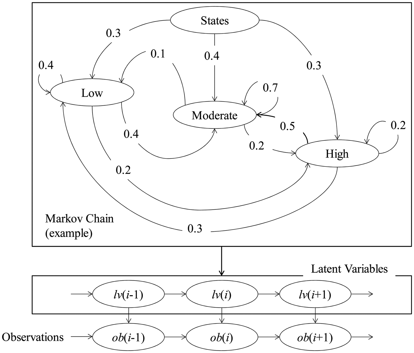
Figure 1 schematically illustrates a hidden Markov model consisting of three modules. The first module is called a Markov chain. The second module is called a time series of latent variables. The last module is called a time series of observations. The descriptions of the three modules are as follows:

Fig. 1. The concept of hidden Markov model.
As seen in Figure 1, a Markov chain forms a network showing both a set of discrete states (which later appear as latent variables) and their transitions. Each state and its possible transitions are associated with the probabilities, which are also the parts of the Markov chain. For example, the Markov chain shown in Figure 1 consists of three discrete states having the probabilities p(Low) = 0.3, p(Moderate) = 0.4, and p(High) = 0.3. The transitions to states denoted as Low, Moderate, and High from the state Low exhibit the following transition probabilities: p(Low|Low) = 0.4, p(Low|Moderate) = 0.4, and p(Low|High) = 0.2. The summation of the state probabilities or the transition probabilities from a given state to other possible states is unit. There are other issues related to the hidden Markov chain (e.g., the order of the Markov chain). The case shown in Figure 1 corresponds to the first order Markov chain because the probability of the previous state determines the current state. This paper adopts this strategy. See Fraser (Reference Fraser2008) and Visser (Reference Visser2011) for more details regarding the order of a Markov chain and other relevant issues.
Regarding the module called time series of the latent variables, the following remarks can be made. The latent variables are the results of a stochastic simulation process (i.e., Monte Carlo simulation of discrete states associated with the Markov chain). Thus, for the case shown in Figure 1, the latent variables belong to the set of discrete states, that is, lv(0),…,lv(i−1), lv(i), lv(i + 1),…∈ {Low, Moderate, High}. These are called latent because one cannot observe (or not interested in observing) these variables, that is, they are simulated for the sake of computation. The probabilities (in reality, relative frequencies) of the latent variables must be consistent with the transition probabilities associated with the Markov chain. This means that for the case shown in Figure 1, when lv(i) = Low, then the probability of lv(i + 1) = Low is equal to 0.4, lv(i + 1) = Moderate is equal to 0.4, and lv(i + 1) = High is equal to 0.2.
Lastly, regarding the module called the time series of the observations, the following remarks can be made. The observations ob(0),…,ob(i−1), ob(i), ob(i + 1),… are simulated using the information of the corresponding latent states, lv(0),…,lv(i−1), lv(i), lv(i + 1),…. The observations are the outputs of the hidden Markov model, which is used to solve a problem.
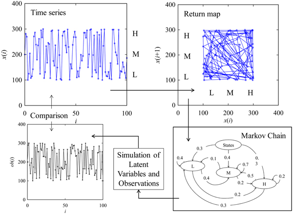
When one constructs a hidden Markov model to encapsulate the dynamics underlying a given time series, the scenario shown in Figure 2 evolves. The scenario entails five steps, namely, data acquisition (defining the time series, return map, and latent variables), Markov chain construction, simulation of latent variables and observations, and a comparison between the simulated observations and given time series. This paper uses the above-mentioned steps for creating a time-series-driven phenomenon twin. For the sake of better understanding, a set of mathematical entities and their relationships are required, which are described in the following subsection.
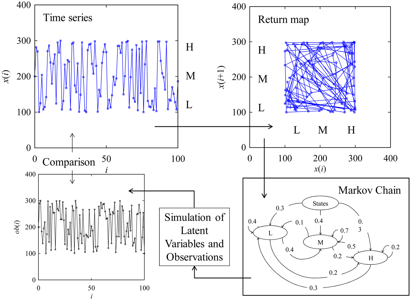
Fig. 2. Integration between hidden Markov model and time series.
Mathematical formulations
This subsection describes the mathematical entities and the underlying relationships that are needed to create a time-series-driven phenomenon twin using a hidden Markov model. The goal is to define the processes underlying the data acquisition, Markov chain construction, simulation of latent variables and observations, and a comparison between simulated observations and given time series.
Let the manifestation of a phenomenon be a piece of time series denoted as X = {x(t) ∈ ℜ | t = 0, Δt, 2Δt,…, m × Δt} where Δt is known as delay or interval. The parameter t underlies a temporal or spatial entity, that is, a point of time or a distance. If preferred, the time series can be represented by indexing its elements using a pointer. In this case, x(t) is replaced by x(i) (=x(t)) where t = i × Δt and i is the pointer, which is an positive integer including 0, that is, i = 0,1,….
Let U = [u min,u max] ∈ ℜ, defined as the universe of discourse, be an interval so that X ⊇ U. Let x min be the minimum value of X, that is, x min = min(x(t) | ∀t ∈{0,Δt, 2Δt,…}). Let x max be the maximum value of X, that is, x max = max(x(t) | ∀t ∈{0, Δt, 2Δt, …}). If U = [u min,u max] = [x min,x max], then it is defined as the exact interval case.
Let U 1, …,U n be n number of mutually exclusive intervals that partition U so that the following proposition denoted as P is true.
 $$P = \left( \matrix{(U_1\cup \ldots \cup U_n = U)\wedge \lpar {U_j \lt U_{\,j + 1}{\rm \vert} \; \forall j\in \lcub {1\comma \, \ldots\comma \, n-1} \rcub } \rpar \hfill \cr \quad \wedge \lpar {U_k\cap U_l = \emptyset \; {\rm \vert} \; \forall k\in \lcub {1\comma \, \ldots\comma \, n} \rcub \comma \,\forall l\in \lcub {1\comma \, \ldots\comma \, n} \rcub -\lcub j \rcub } \rpar \hfill} \right)$$
The partitions are the states (or latent states or variables) of X resulting in a state vector SV = (U 1,…,U n). One can define the states in many ways making the proposition P true. One of the straightforward ways is to consider a state interval Δu = (u max−u min)/n and use it for defining the states in the following manner: U 1 = [u min, u min + Δu), U 2 = [u min + Δu, u min + 2Δu), …, U n = [u min + (n−1) × Δu, u min + n × Δu].
Let p(U j) ∈ [0,1] be the probability of j-th state U j in SV with respect to X, j = 1,…,n. Thus, the following relationship holds.
 $$\Phi (x(i)\comma \,U_j) = \left\{ {\matrix{ {1\comma \,\; \; x(i) \in U_j} \cr {0\comma \,\; \; {\rm otherwise}} \cr}} \right.$$
 $$p(U_j) = \displaystyle{{\mathop \sum \nolimits_{i = 0}^m \Phi \lpar {x(i)\comma \,U_j} \rpar } \over {m + 1}}$$
Thus, p(U j) is defined as the state probability of the j-th state U j. As such, the summation of all state probabilities is equal to unit, that is,
 $$p(U_1) + \ldots + p(U_n) = 1$$
For the sake of computation (e.g., simulation), the state probabilities can be used to calculate the cumulative state probability. The cumulative state probability of the j-th state U j in SV is defined as follows:
 $${pc}(U_j) = p(U_1) + \ldots + p(U_j)$$
As such, pc(U n) = 1. The cumulative state probability can be used to calculate the state probability interval denoted as pc in(U j). The state probability interval of the first state U 1 in SV is as follows:
 $${p}{\rm c}_{{\rm in}}(U_1) = [ {0\comma \,{pc}(U_1)} \rpar $$
The state probability interval of the last state U n in SV is as follows:
 $${pc}_{{\rm in}}(U_n) = [ {{pc}(U_{n-1})\comma \,{pc}(U_n)} ] $$
The state probability intervals of the states other than U 1 and U n in SV are as follows:
 $${p}{\rm c}_{{\rm in}}(U_j) = [ {{pc}(U_{\,j-1})\comma \,{pc}(U_j)} \rpar \quad \forall j\in \{ 2\comma \, \ldots\comma \, n-1\} $$
Let the set of tuples {(x(i),x(i + 1)) | i = 1,2,…} (or {(x(t),x(t + iΔt)) | i = 1,2,…}) be the return or delay map of the time series X. Therefore, each point (x(i), x(i + 1)), ∃i ∈ {1,2,…} of the return map exhibits a transition. As a result, a transition probability denoted as tp(U o| U j) (∀o, ∀j ∈{1,…,n}) means the likelihood of the transition of X to the state U o from the state U j. Thus, the following relationships hold.
 $$\Phi ((x(i){\rm ,} x(i + 1)){\rm ,} (U_o{\rm ,} U_j)) = \left\{ {\matrix{ {1,} & {((x(i)\in U_j)\wedge (x(i + 1)\in U_o))} \cr {0,} & {{\rm otherwise}} \hfill \cr } } \right.$$
 $${tp}(U_o \vert U_j) = \displaystyle{{\mathop \sum \nolimits_{i = 0}^m \Phi \lpar {\lpar {x(i)\comma \,x(i + 1)} \rpar \comma \,(U_o\comma \,U_j)} \rpar } \over {\mathop \sum \nolimits_{i = 0}^m \Phi \lpar {x(i)\comma \,U_j} \rpar }}$$
As such, the summation of all transition probabilities from a given state is equal to unit, that is, tp(U 1|U j) + … + tp(U n|U j) = 1, ∃j ∈ {1,…,n}. This yields a transition probability matrix as follows:
 $$M_{{tp}} = \left[ {\matrix{ {{tp}(U_1 \vert U_1)} & \cdots & {{tp}(U_n \vert U_1)} \cr \vdots & \ddots & \vdots \cr {{tp}(U_1 \vert U_n)} & \cdots & {{tp}(U_n \vert U_n)} \cr}} \right]$$
For the sake of computation (e.g., simulation), the transition probabilities can be used to calculate the cumulative transition probability. The cumulative transition probability is defined as follows:
 $${tpc}(U_o \vert U_j) = {tp}(U_1 \vert U_j) + \ldots + {tp}(U_o \vert U_j)$$
As such, tpc(U n|U j) = 1. This yields the cumulative transition probability matrix, as follows:
 $$M_{{tpc}} = \left[ {\matrix{ {{tpc}(U_1 \vert U_1)} & \cdots & {{tpc}(U_n \vert U_1)} \cr \vdots & \ddots & \vdots \cr {{tpc}(U_1 \vert U_n)} & \cdots & {{tpc}(U_n \vert U_n)} \cr}} \right]$$
The cumulative transition probability can be used to calculate the transition probability interval denoted as tpc in(U o|U j). The transition probability interval of the first states U 1 to any state U j is as follows:
 $${tpc}_{{\rm in}}(U_1 \vert U_j) = [ {0\comma \,{tpc}\lpar {U_1 \vert U_j} \rpar } \rpar $$
The transition probability interval of the last state U n to any state U j is as follows:
 $${tpc}_{{\rm in}}(U_n \vert U_j) = [ {{tpc}(U_{n-1} \vert U_j)\comma \,{tpc(}U_n \vert U_j{\rm )}} ] \; $$
The transition probability intervals of any states to U j (other than U 1 or U n) are as follows:
 $$\eqalign{tpc_{{\rm in}}(U_o|U_j) &= [tpc(U_{o-1}|U_j){\rm ,}tpc(U_o|U_j))\forall o \cr & \in \{ 2{\rm ,} \ldots {\rm ,} n-1\} } $$
Simulation
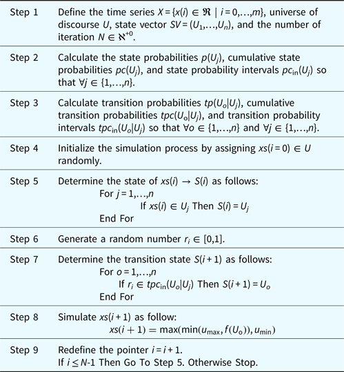
Using the mathematical entities and their relationships described in the previous subsection, one can formulate a Monte Carlo simulation process to simulate the latent variables lv(·) ∈ (U 1,…,U n) and the observations ob(·) ∈ ℜ. Note that the simulated observations will be denoted as xs(·), not as ob(·), to make the notation consistent with the time series, x(·). The simulation process consists of the following nine steps. The first three steps, Steps 1,…,3, are related to the steps of the Markov chain formulation as shown in Figure 2. The other steps, Steps 4,…,9, are related to the steps of the simulation of latent variables and observations as shown in Figure 2.
Note that in Step 8, a function f(U (·)) is introduced. It produces a value based on the state U (·). When any other information is not available, f(U (·)) randomly generates a real number from a normally distributed variable denoted as rn (·)(μ(U (·)),σ(U (·))). Here, μ(U (·)) and σ(U (·)) denote the mean and standard deviation, respectively. As such, the following formulation holds:
 $$f\,(U_{(\cdot )}) = {rn}_{(\cdot )}((\mu _{(\cdot )})\comma \,(\sigma _{(\cdot )}))$$
The formulation of f(U (·)) defined in (12) is used in this article. [Other formulations of f(U (·)) can be used, as preferred].
It is worth mentioning that even though a simulated value xs(i) belongs to one of the states say U j, the next state xs(i + 1) may not belong to the same state. This means that the simulation process continues similar to a dynamical system (Ullah, Reference Ullah2017).
However, since the intention of constructing the hidden Markov model is to encapsulate the dynamics of the stochastic features underlying the given time series, the given time series X = {x(i) ∈ ℜ | i = 0,…,m} and the simulated time series S = {xs(i) ∈ ℜ | i = 0,1,…} must exhibit similar characteristics. The parameters by which one quantifies the characteristics depend on the phenomenon involved with the given time series X. In general, at least one parameter is needed to compare X and S in the time domain. In addition, one parameter is needed to quantify them in delay domain, that is, their return maps {(x(i),x(i + 1)) | i = 0,1,…,m−1} and {(xs(i),xs(i + 1)) | i = 0,1,…}. However, one of the default choices by which one can compare the characteristics of X and S is an entity that is probability distribution-neutral representation of the uncertainty associated with X and S. Since a possibility distribution (e.g., a fuzzy number) is a probability distribution-neutral representation of the uncertainty, the possibility distributions induced from X and S can be used to compare them. The description of the induction of a fuzzy number (i.e., a possibility distribution) from a given set of data can be found in Ullah and Shamsuzzaman, Reference Ullah and Shamsuzzaman2013.
Case Study
The computing power of hidden Markov models has been playing an important role in studying the complex phenomena underlying design and manufacturing. For example, Liao et al. (Reference Liao, Li and Cui2016) have developed a heuristic optimization algorithm using hidden Markov model coupled with simulated annealing for condition monitoring of machineries. Li et al. (Reference Li, Fang, Huang, Wei and Zhang2018) have developed a data-driven bearing fault identification methodology using an improved hidden Markov model and self-organizing map. Mba et al. (Reference Mba, Makis, Marchesiello, Fasana and Garibaldi2018) developed a hidden Markov model-based methodology for condition monitoring of gearbox. Zhang et al. (Reference Zhang, Zhang and Zhu2018) developed a methodology for predicting the residual life of the rolling machine elements using hidden Markov model. Xie et al. (Reference Xie, Hu, Wu and Wang2016) described the hidden Markov model-based methodology for recognizing the machining states ensuring safe operations. Bhat et al. (Reference Bhat, Dutta, Pal and Pal2016) developed a hidden Markov model-based tool condition monitoring methodology ensuring the economical usages of cutting tools. Liao et al. (Reference Liao, Hua, Qu and Blau2006) developed a grinding wheel condition monitoring methodology where a hidden Markov model-based clustering approach was used to recognize the patterns found in the acoustic emission signals. Cai et al. (Reference Cai, Shi, Shao, Wang and Liao2018) developed a methodology using a hidden Markov model to identify the energy efficiency states while removing materials by milling ensuring eco-friendly machining operation. Kumar et al. (Reference Kumar, Chinnam and Tseng2018) integrated hidden Markov model with polynomial regression for predicting the useful life of cutting tools. Nevertheless, this case study shows how to apply the hidden Markov model (presented in the section “Methodology”) for constructing a phenomenon twin of surface roughness. The description is as follows.
Surface roughness is a concept used to quantify the degree of the surface finish of a processed surface. Therefore, when one studies a manufacturing process in laboratory settings, the surface heights data are measured by using appropriate surface metrology equipment. Afterward, the measured surface heights data are processed to calculate different types of parameters for quantifying the surface roughness. A description of how the surface height data should be processed for calculating the conventional and nonconventional surface roughness quantification parameters can be found in Ullah et al. (Reference Ullah, Fuji, Kubo, Tamaki and Kimura2015). On the other hand, when one monitors a manufacturing process in real-life settings, the surface heights data are measured by using an appropriate sensor-driven system. The surface heights data are then processed to know whether the process produces the expected surface roughness. As far as the data processing is concerned, the surface heights data are a piece of time series. These data can be processed by using different approaches for the reconstruction of the surface heights [e.g., fractional Brownian motion-based simulation (Higuchi et al., Reference Higuchi, Yamaguchi, Yano, Yamamoto, Ueshima, Matumori and Yoshizawa2001), rule-based systems (Ullah and Harib, Reference Ullah and Harib2006), autocorrelation analysis (Chui et al., Reference Chui, Feng, Wang, Li and Li2013; Choi et al., Reference Choi, Shi, Lowe, Skelton, Craster and Daniels2018), feature-based simulation (Ullah et al., Reference Ullah, Tamaki and Kubo2010), and integer-sequencedbased dynamical systems (Ullah, Reference Ullah2017)]. The methodologies mentioned above are highly customized, and require a large set of user-defined parameters. Thus, for simplifying the process of the reconstruction of the surface heights, one can use the hidden Markov model described in the previous section. This possibility is explored using the case of surface heights of ground surfaces (i.e., surfaces heights generated due to the application of a material removal process called grinding).
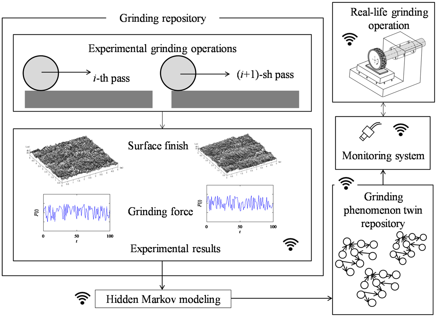
Grinding is a widely used material removal process that helps remove materials from the surfaces of the objects made of difficult-to-cut materials (e.g., stainless steels, ceramics, and so forth) ensuring a high surface finish. In grinding, a complex microscopic interaction between the abrasive grains attached on the circumferential surface of grinding wheel and work-surface takes place (Ullah et al., Reference Ullah, Caggiano, Kubo and Chowdhury2018). As a result, in a grinding operation, a grinding wheel passes the same area of the work surface multiple times (as schematically illustrated in Fig. 3) so that the desired amount of materials is removed and better surface finish is achieved. This results in a gradual change in the surface roughness. A detailed description of this grinding mechanism can be found in Ullah et al. (Reference Ullah, Caggiano, Kubo and Chowdhury2018).

Fig. 3. An architecture of hidden Markov model-based grinding operation system.
Now, from the viewpoint of futuristic manufacturing systems, one can consider that there is a repository defined as the grinding experiment repository where the pass-by-pass grinding experiment results are stored for reuse, as schematically illustrated in Figure 3. It can be located in the manufacturing clouds for sharing as described by Wu et al. (Reference Wu, Terpenny and Schaefer2016). Nevertheless, using the information stored in the grinding experiment repository, one can construct the digital twins of grinding phenomena (e.g., the digital twins of the grinding force, grinding temperature, wear of grinding wheel, surface roughness, and so forth). This way, the user-dependency can be reduced in manufacturing clouds. As a result, the digital twins form another repository defined as the grinding phenomenon twin repository. Between these two repositories, the hidden Markov model plays its role as schematically illustrated in Figure 3. This means that some of the phenomena twins are constructed by using the hidden Markov model. It is worth mentioning that similar repositories can be built for other manufacturing processes, too, and placed in the manufacturing clouds. This will help make the manufacturing clouds more functional because manufacturing clouds still have limited usability since solving modeling and simulations problems in manufacturing clouds depends heavily on the user-experience (Wu et al., Reference Wu, Terpenny and Schaefer2016).
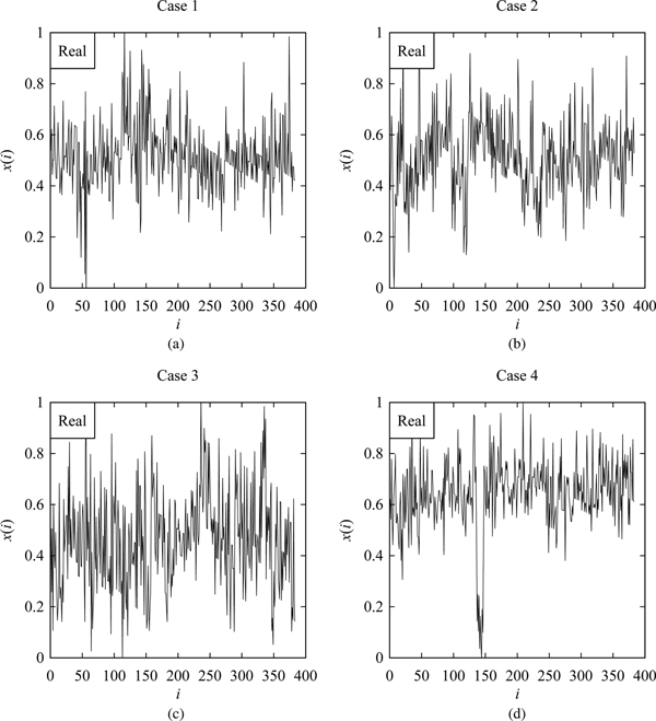
To see the efficacy of the hidden Markov model in creating a phenomenon twin of the surface roughness of grinding operations, consider the measured surface heights of a ground surface for the four consecutive passes, denoted as Cases 1,…,4 as reported in Ullah et al. (Reference Ullah, Caggiano, Kubo and Chowdhury2018). For the sake of comparison, the heights are normalized and shown by the four plots in Figure 4. As seen in Figure 4, the surface heights are very irregular and stochastic. For constructing a hidden Markov model, the following five latent states are considered making the proposition P true [Eq. (1)]: U 1 = [0,0.2), U 2 = [0.2,0.4), U 3 = [0.4,0.6), U 4 = [0.6,0.8), and U 5 = [0.8,1], that is,  ${U_1} \cup U_2 \cup U_3 \cup U_4 \cup &InLnBrk;U_5 = [ {0\comma \,1} ] .$ From the semantics sense, “U 1” represents “very low” heights, “U 2” represents “low” heights, “U 3” represents “moderate” heights, “U 4” represents “high” heights, and “U 5” represents “very high” heights. A user may use other formulations of the latent states.
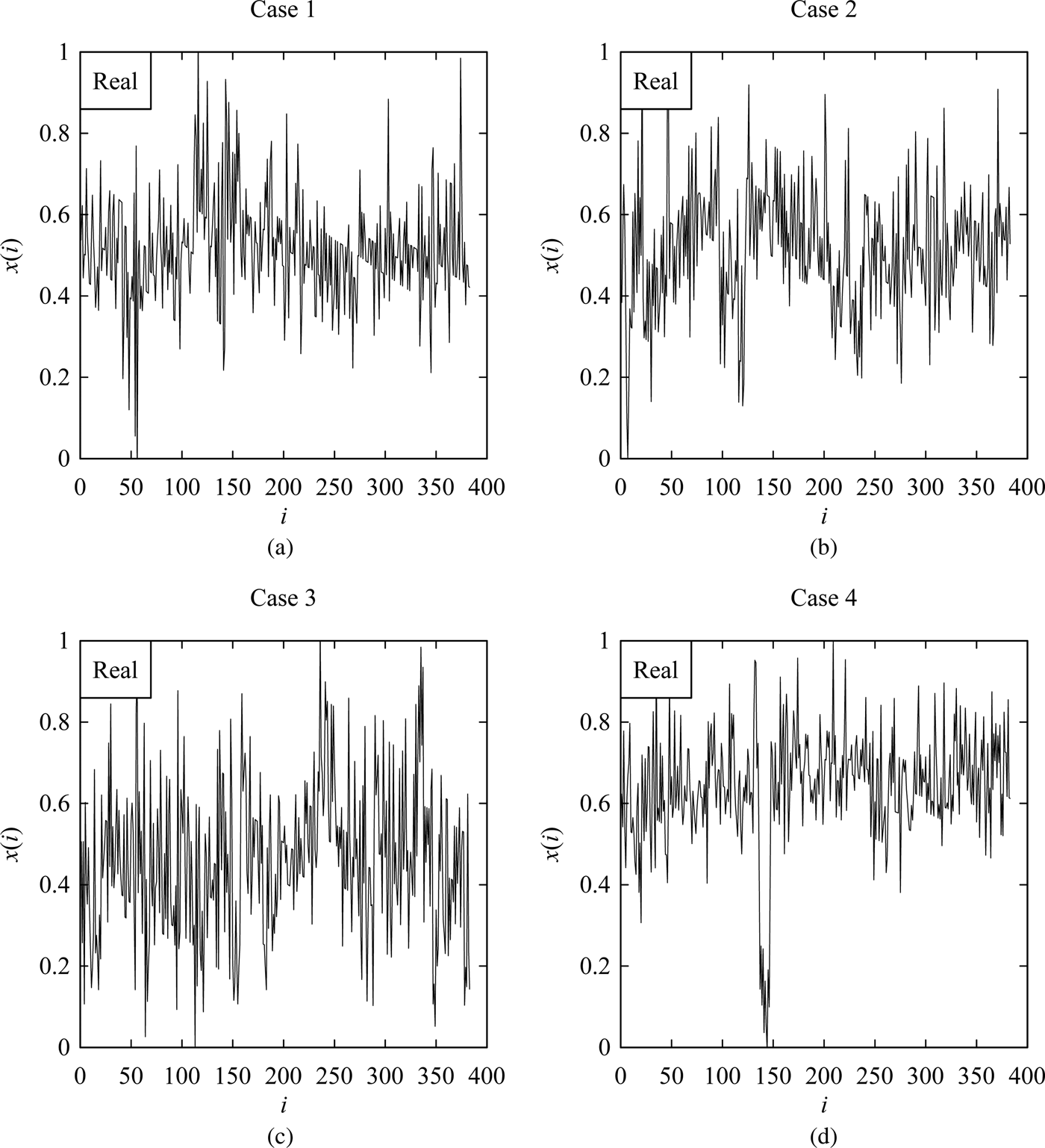
Fig. 4. The normalized ground surface heights (Ullah et al., Reference Ullah, Caggiano, Kubo and Chowdhury2018). (a) Measured surface heights after the first pass. (b) Measured surface heights after the second pass. (c) Measured surface heights after the third pass. (d) Measured surface heights after the fourth pass.
In accordance with Eq. (9), the transition probability matrix (M tp) for Cases 1,…,4 are constructed as given by Eqs (13)–(16).
 $$M_{{tp}\lpar {{\rm Case\;} 1} \rpar } = \left[ {\matrix{ 0 & {0.5} & {0.25} & {0.25} & 0 \cr 0 & {0.192} & {0.577} & {0.212} & {0.019} \cr {0.004} & {0.142} & {0.696} & {0.130} & {0.028} \cr {0.043} & {0.058} & {0.594} & {0.275} & {0.030} \cr 0 & {0.091} & {0.273} & {0.545} & {0.091} \cr}} \right]$$
 $$M_{{tp}\lpar {{\rm Case}\; 2} \rpar } = \left[ {\matrix{ {0.333} & {0.334} & {0.333} & 0 & 0 \cr {0.044} & {0.324} & {0.5} & {0.117} & {0.015} \cr {0.010} & {0.171} & {0.540} & {0.245} & {0.034} \cr {0.011} & {0.078} & {0.555} & {0.323} & {0.033} \cr 0 & {0.083} & {0.584} & {0.25} & {0.083} \cr}} \right]$$
 $$M_{{tp}\lpar {{\rm Case}\; 3} \rpar } = \left[ {\matrix{ {0.290} & {0.291} & {0.161} & {0.161} & {0.097} \cr {0.135} & {0.288} & {0.406} & {0.144} & {0.027} \cr {0.032} & {0.31} & {0.478} & {0.154} & {0.026} \cr {0.045} & {0.258} & {0.409} & {0.182} & {0.106} \cr 0 & {0.2} & {0.2} & {0.45} & {0.15} \cr}} \right]$$
 $$M_{{tp}\lpar {{\rm Case\;} 4} \rpar } = \left[ {\matrix{ {0.625} & {0.25} & {0.125} & 0 & 0 \cr {0.4} & 0 & {0.2} & {0.4} & 0 \cr {0.009} & {0.009} & {0.375} & {0.5} & {0.107} \cr 0 & {0.009} & {0.257} & {0.635} & {0.099} \cr 0 & 0 & {0.306} & {0.638} & {0.056} \cr}} \right]$$
In accordance with Eq. (11), the cumulative transition probability matrix (M tpc) for Cases 1,…,4 are constructed as given by Eqs (17)–(20).
 $$M_{{tpc}\lpar {{\rm Case}\; 1} \rpar } = \left[ {\matrix{ 0 & {0.5} & {0.75} & 1 & 1 \cr 0 & {0.192} & {0.769} & {0.989} & 1 \cr {0.004} & {0.146} & {0.842} & {0.972} & 1 \cr {0.043} & {0.101} & {0.695} & {0.970} & 1 \cr 0 & {0.091} & {0.364} & {0.909} & 1 \cr}} \right]$$
 $$M_{{tpc}\lpar {{\rm Case}\; 2} \rpar } = \left[ {\matrix{ {0.333} & {0.667} & 1 & 1 & 1 \cr {0.044} & {0.368} & {0.868} & {0.985} & 1 \cr {0.010} & {0.181} & {0.721} & {0.966} & 1 \cr {0.011} & {0.089} & {0.644} & {0.967} & 1 \cr 0 & {0.083} & {0.667} & {0.917} & 1 \cr}} \right]$$
 $$M_{{tpc}\lpar {{\rm Case}\; 3} \rpar } = \left[ {\matrix{ {0.290} & {0.581} & {0.742} & {0.903} & 1 \cr {0.135} & {0.423} & {0.829} & {0.973} & 1 \cr {0.032} & {0.342} & {0.820} & {0.974} & 1 \cr {0.045} & {0.303} & {0.712} & {0.894} & 1 \cr 0 & {0.2} & {0.4} & {0.85} & 1 \cr}} \right]$$
 $$M_{{tpc}\lpar {{\rm Case}\; 4} \rpar } = \left[ {\matrix{ {0.625} & {0.875} & 1 & 1 & 1 \cr {0.4} & {0.4} & {0.6} & 1 & 1 \cr {0.009} & {0.018} & {0.393} & {0.893} & 1 \cr 0 & {0.009} & {0.266} & {0.901} & 1 \cr 0 & 0 & {0.306} & {0.944} & 1 \cr}} \right]$$
Using the results shown in Eqs (17)–(20), the transition probability intervals denoted as tpc in(U o|U j) (∀o ∈ {1,…,5} and ∀j ∈ {1,…,5}) are calculated for each case. For simulating the observations from the latent states, the values of the mean of the respective states are set as follows: μ(U 1) = 0.1, μ(U 2) = 0.3, μ(U 3) = 0.5, μ(U 4) = 0.7, and μ(U 5) = 0.9. The values of the standard deviation are set as follows: σ(U 1) = σ(U 2) = σ(U 3) = σ(U 4) = σ(U 5) = 0.05. This formulation is based on Eq. (12). Using the above settings, the Monte Carlo simulations as defined by Steps 4,…,9 (see the section “Simulation”) are carried out for each case. Figure 5 shows the screen-print of the spreadsheet-based computing tool that implements the simulation process. As seen in Figure 5, the real surface heights X (in this case see Case 4 in Fig. 4) and the simulated surface heights S are seen on the screen-print. The user needs to input the time series X and define the latent states, U 1,…,U 5. The computing tool does the rest. The computing tool also plots the respective return maps and the possibility distributions for the sake of comparison.
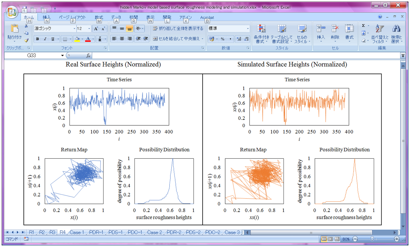
Fig. 5. Computing tool for implementing hidden Markov model-based surface roughness modeling and simulation.
However, Figures 6–9 shows the samples of the simulated surface heights in terms of both time series and return maps, along with the time series and return maps of the respective real heights. For comparing the characteristics of real surface heights X and simulated surface heights S, two parameters are considered in this section. The first parameter is the arithmetic mean deviation of the surface heights denoted as Ra (Ullah et al., Reference Ullah, Fuji, Kubo, Tamaki and Kimura2015), which is the most widely used surface roughness parameter. The other one is the possibility distributions (or fuzzy numbers) (Ullah and Shamsuzzaman, Reference Ullah and Shamsuzzaman2013).

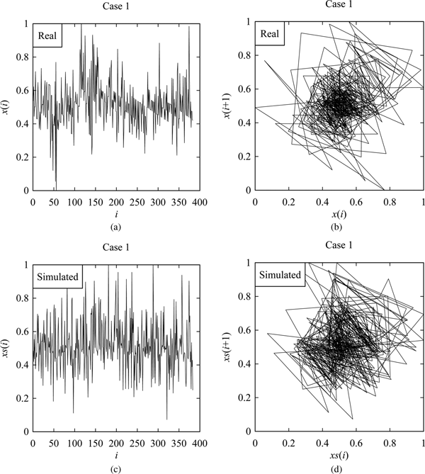
Fig. 6. Results corresponding to Case 1. (a) Real surface profile. (b) Return map of (a). (c) Simulated surface profile. (d) Return map of (c).
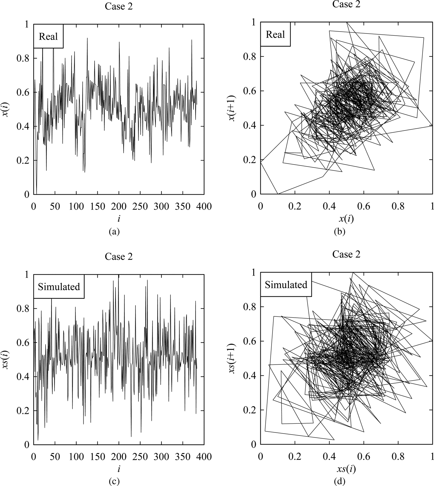
Fig. 7. Results corresponding to Case 2. (a) Real surface profile. (b) Return map of (a). (c) Simulated surface profile. (d) Return map of (c).
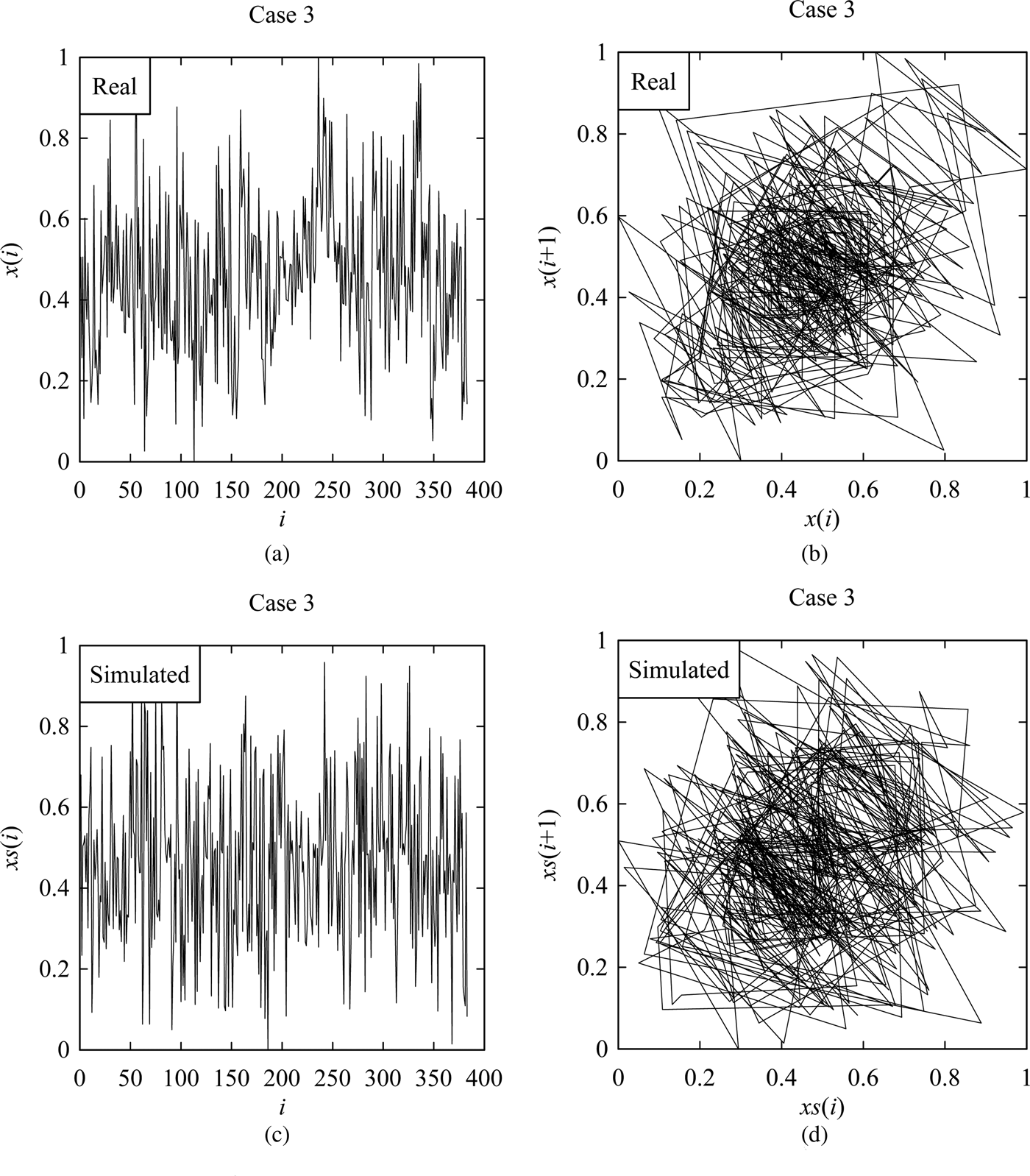
Fig. 8. Results corresponding to Case 3. (a) Real surface profile. (b) Return map of (a). (c) Simulated surface profile. (d) Return map of (c).
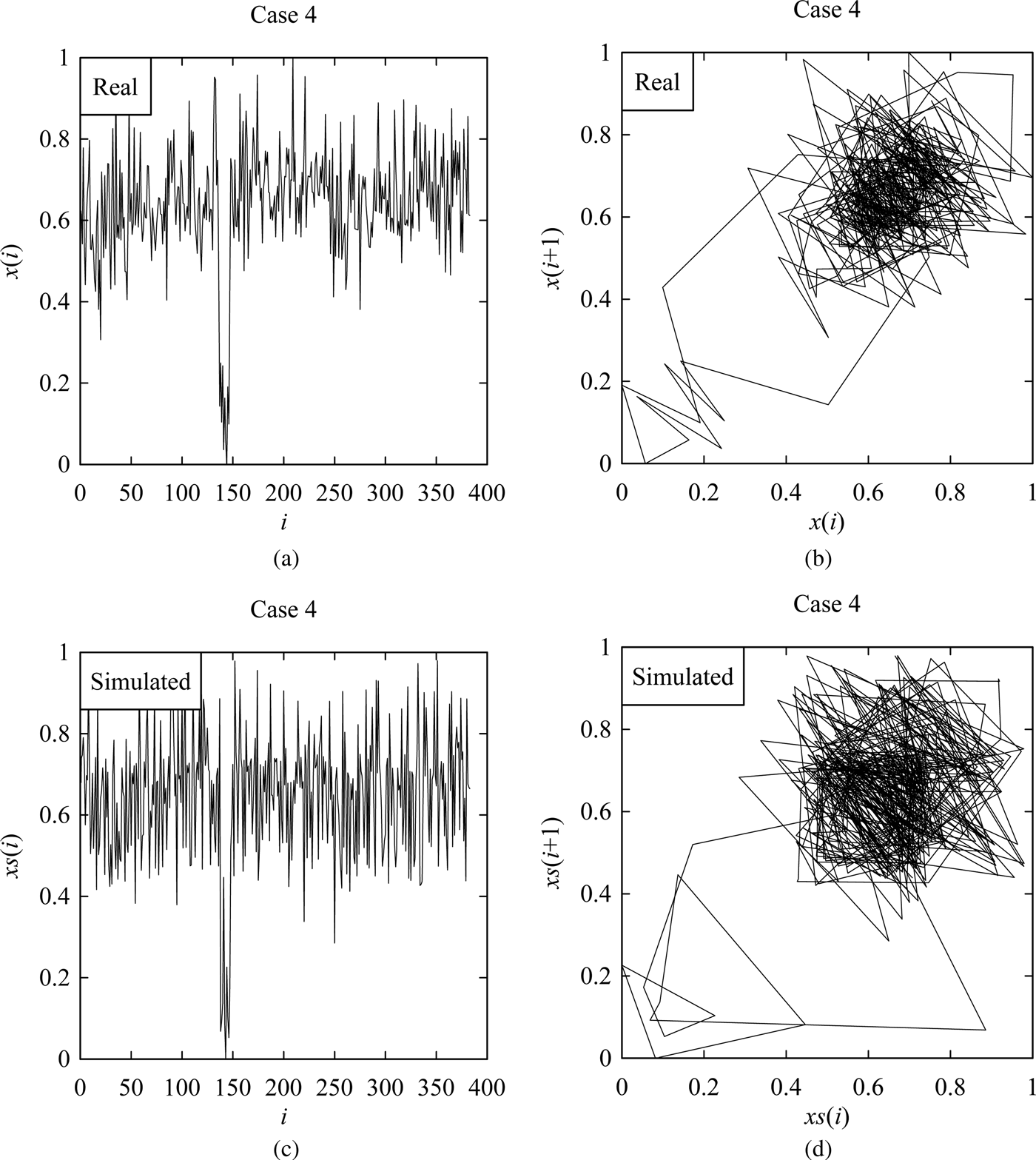
Fig. 9. Results corresponding to Case 4. (a) Real surface profile. (b) Return map of (a). (c) Simulated surface profile. (d) Return map of (c).
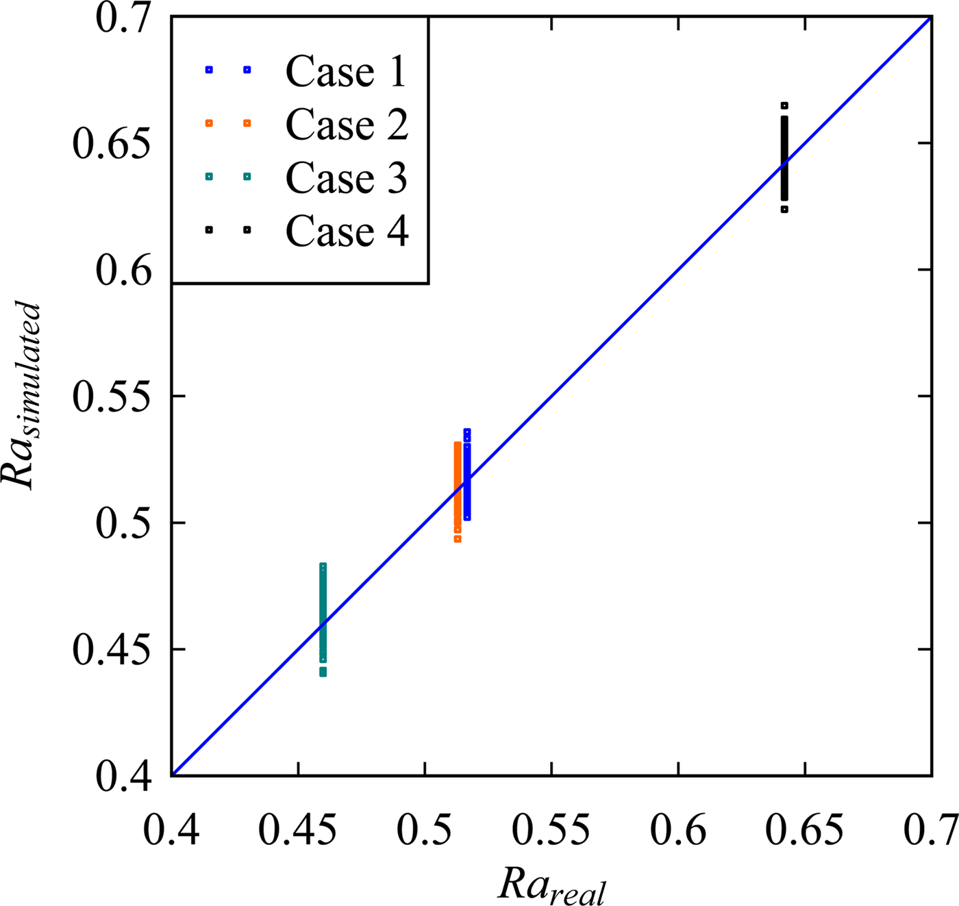
The values of Ra are calculated for the real and simulated surface heights (i.e., for X and S) as shown in Figure 10. The simulations were carried out 100 times for each case to observe the variability. The unit-sloped straight line shown by the blue color in Figure 10 represents the ideal case, that is, Ra of the simulated surface heights is equal to that of the real surface heights. As seen in Figure 10, for all cases, more than 50% of the simulated results are greater than that of the real ones. This means that the hidden Markov model-based phenomenon twin for surface roughness produces a rougher surface than the real one.

Fig. 10. Comparison between the real and the simulated surface roughness.
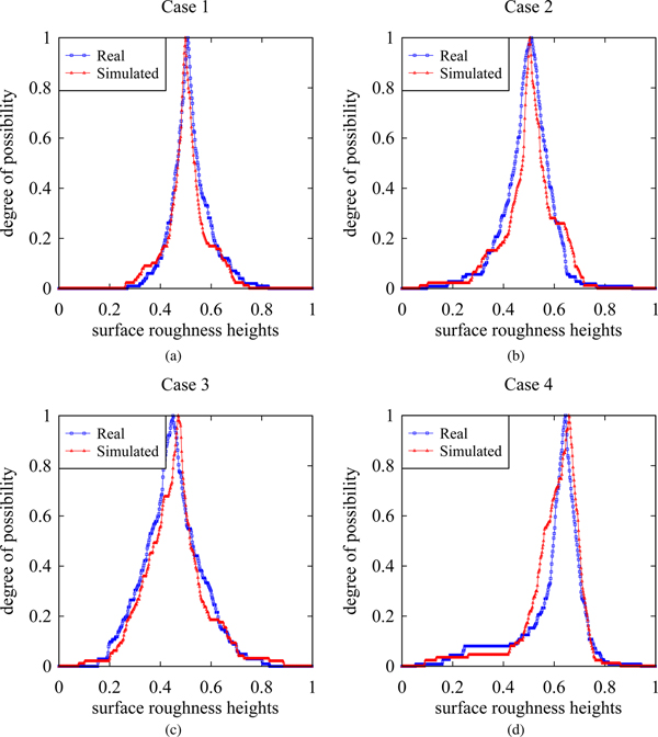
On the other hand, the possibility distributions of the simulated surface heights resemble those of the real surface heights, as shown in Figure 11. This means that from the dynamical systems point of view, the characteristics of the real and simulated surface heights are quite similar although their degrees of roughness are not exactly the same.
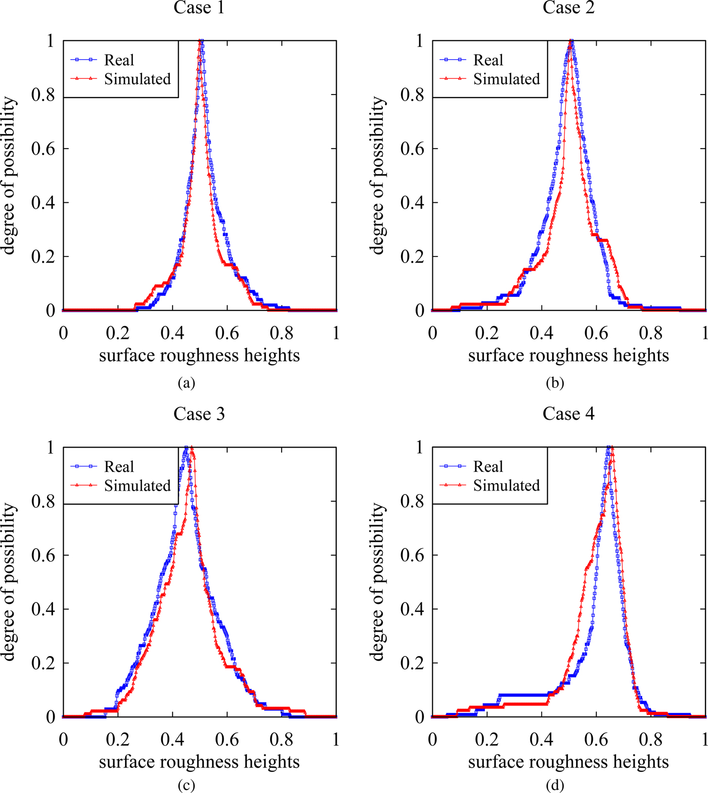
Fig. 11. Possibility distributions of the real and the simulated surface heights. (a) Case 1. (b) Case 2. (c) Case 3. (d) Case 4.
Ontology
Apart from the comparison between the real and simulated surface heights, there are other important issues, for example, the issue of ontology. Ontology has been implemented within the framework of futuristic manufacturing systems, for example, see the articles Khilwani and Harding (Reference Khilwani and Harding2014), Ramos (Reference Ramos2015), Lu and Xu (Reference Lu and Xu2018), Kim and Ahmed (Reference Kim and Ahmed2018). It provides a semantic representation of the relevant contents. It has become more relevant because of both the maturity indices of the web technology (semantic web or web 3.0/4.0, e.g., see Berners-Lee et al., Reference Berners-Lee, Hendler and Lassila2001) and the futuristic manufacturing systems (understand, predict, decide, and adopt, e.g., see Schuh et al., Reference Schuh, Anderl, Gausemeier, Hompel and Wahlster2017). In terms of the enterprise system architecture, an ontology is a semantic model of the contents (e.g., in this case, a semantic model of the digital twin) that forms the meta-model and meta-meta model (Tunjic et al., Reference Tunjic, Atkinson and Draheim2018), that is, high-level description of the contents. Therefore, the semantic annotations (linguistically described semantic description) must accompany all concepts necessary for encoding the contents (Fill, Reference Fill2017, Reference Fill2018). On the other hand, as far as the semantic web—which will be used to functionalize the connections of cyber-physical systems (Alam and Saddik, Reference Alam and Saddik2017)—is concerned, the role of the ontology can be seen from a broader perspective. Compared to its predecessors (web 1.0/2.0), the semantic web has some additional features that make it self-contained and autonomous. These features form the upper layers of the semantic web layer-cake, namely, unified logic, proof, trust, and user-interface and application (Sizov, Reference Sizov2007). The purpose of these layers is to provide the provenance (Moreau et al., Reference Moreau, Groth, Cheney, Lebo and Miles2015; Oliveira et al., Reference Oliveira, Ambrósio, Braga, Ströele, David and Campos2017) of the contents, incorporating the individuals, institutions, data sources, data manipulation methodologies and algorithms, and so forth regarding the contents. Using the provenance, the layers of unified logic, proof, trust, and user-interface are built. Therefore, an entity defined as meta-ontology, must be made available to the systems developers of the cyber-physical systems using which the developers then construct the ontology of the contents to be used in the upper layers of semantic web layer-cake. Now the question is: what is the meta-ontology of the digital twin of surface roughness? One of the answers is presented as follows:
For the case shown in this section (i.e., digital twin of surface roughness) that entities that are subject to the provenance are as follows: a grinding operation, grinding wheel, workpiece, grinding conditions, surface metrology instrument, grinding machine, computing tool, surface heights, hidden Markov model, digital twin, surface roughness, five latent states, very low, low, moderate, high, very high, state probabilities, transition, one of the latent states, and transition probabilities. These entities can be considered the concepts of a concept map (Ullah et al., Reference Ullah, Arai and Watanabe2013; Ullah, Reference Ullah2019) for providing the meta-ontology of the provenance. One of the possible outcomes is shown in Figure 12. Some of the concepts are repeated (e.g., surface heights) for the sake of better understanding. One can access this concept map from the following URL for integrating it to the systems of futuristic manufacturing systems: http://cmapspublic3.ihmc.us/rid=1SVM7NWKX-W2MYVP-1FWD/hidden-markov-model-of-surface-roughness.cmap. The meta-ontology shown in Figure 12 entails the following propositions: (1) a grinding operation entails a grinding wheel, workpiece, grinding conditions, surface metrology instrument, grinding machine; (2) surface metrology instrument measures the surface heights to represent surface roughness; (3) surface heights are normalized to construct a digital twin of surface roughness using hidden Markov model; (4) hidden Markov model consists of five latent states namely very low, low, moderate, high, and very high; (5) five latent states namely very low, low, moderate, high, and very high have the state probabilities; (6) transition of surface heights from one of the latent states to very low, low, moderate, high, and very high have transition probabilities; (7) hidden Markov model results in a computing tool to simulate surface heights. Each concept can be integrated with other concepts for making it comprehensible to the users who are not familiar to it. For example, with the concept of grinding wheel one can link a concept map that describes a grinding wheel and its features, construction, and so forth. The concept “hidden Markov model” can be linked to the articles or tutorials where a lucid and user-friendly description of it is available. The concept “computing tool” can be linked to a source from where the user can download the computing tool (e.g., the tool shown in Fig. 5). For more details on how to construct a good ontology for manufacturing, refer to Ullah (Reference Ullah2019). It is worth mentioning that one can easily create the machine-readable data (XML, OWL, and so forth) from the concept map shown in Figure 12.
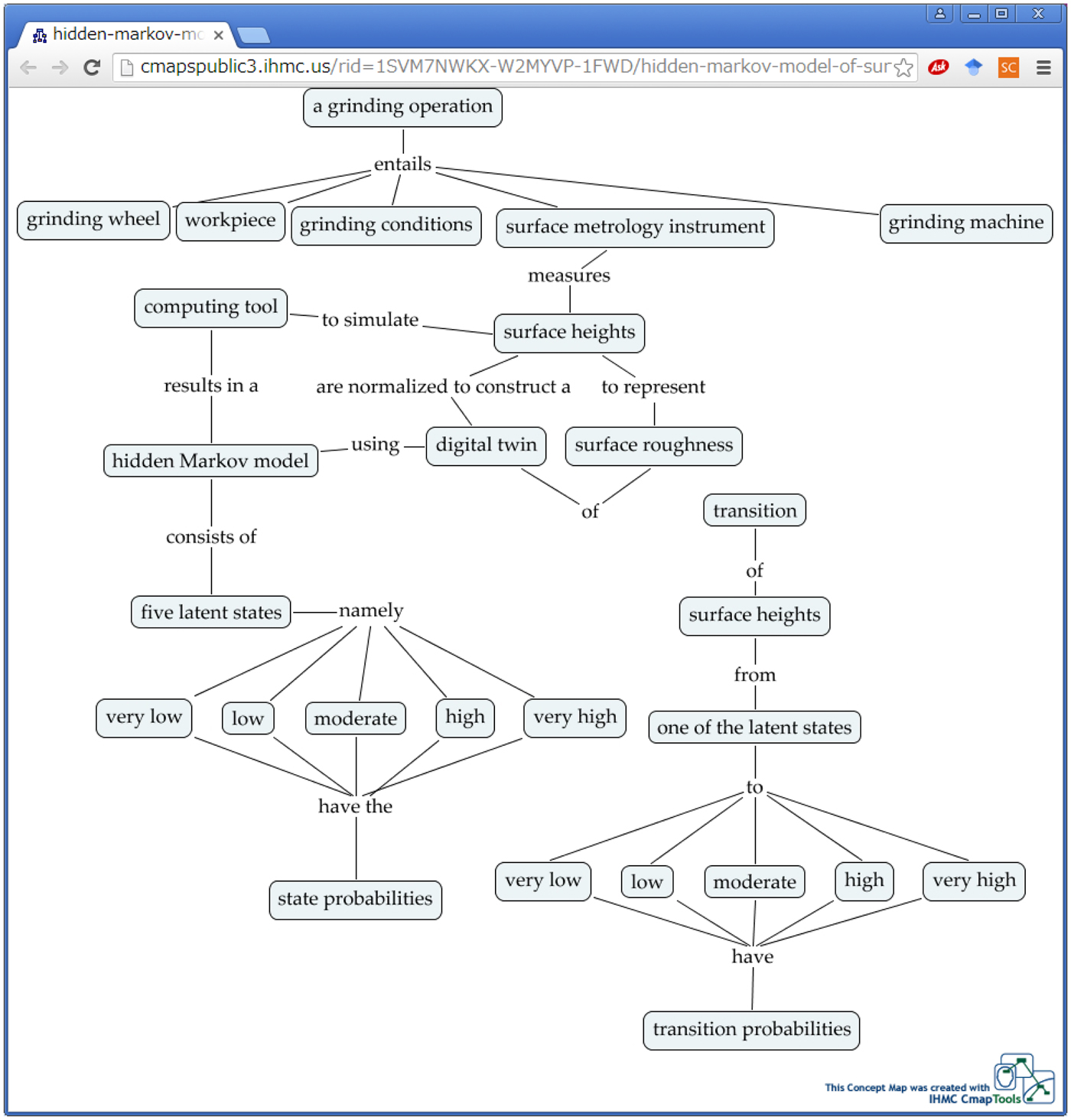
Fig. 12. The meta-ontology of the digital twin of the surface roughness due to grinding.
Summary and concluding remarks
(1) The recent literature review on digital twins relevant to manufacturing suggests that digital twins must populate the cyberspace of the cyber-physical systems to functionalize the futuristic manufacturing systems. This means that the digital twins are the contents on which the systems associated with futuristic manufacturing systems (e.g., cyber-physical systems) act to perform the desired functions. It is however difficult to prescribe a unified methodology by which all kinds of digital twins can be created, used, and managed. This is somewhat a new topic for the manufacturing research community.
(2) As far as the complex phenomena are concerned, the hidden Markov model is one of the choices using which one can construct digital twins. A hidden Markov model consists of three components, namely, a Markov chain, a simulation process that simulates the latent states, and a simulation process that simulates the observation.
(3) It is possible to encapsulate the dynamics of the phenomenon (manifested in the form of a time series) using a Markov chain where the latent states are user-defined. Using a Monte Carlo simulation process, the latent states can be simulated in accordance with the Markov chain. Each simulated latent state can be translated into an observation (i.e., a numerical value) using a user-defined function. The simulated observations (a time series) are the outcomes of the hidden Markov model. If the time series of the observation resembles that of the phenomenon in both qualitative and quantitative viewpoints, then it can be claimed that the constructed hidden Markov model is an exact mirror image of the underlying phenomenon, that is, it is phenomenon twin.
(4) The presented hidden Markov model is applied to construct a digital twin of the surface roughness of a ground surface (a surface created due to successive grinding operations). The surface heights given in the form of a time series is first used to construct a Markov chain using the five latent states (very low heights, low heights, moderate heights, high heights, and very high heights). Using a Monte Carlo simulation process that simulates the latent states in accordance with the constructed Markov chain, the five latent states are simulated randomly to produce a time series of latent states. Each latent state is then translated to an observation (i.e., a simulated surface height) considering that the height distribution follows a normal distribution. The mean and standard deviation are customized for each latent state. The time series of the simulated surface heights and the real surface heights are compared quantitatively using two parameters, i.e., arithmetic average surface roughness (Ra) and possibility distribution (probability-distribution neutral quantification of uncertainty). In terms of Ra, it is found that the hidden Markov model-based phenomenon twin of surface roughness produces a rougher surface than the real one. And, the possibility distributions of the simulated surface heights resemble those of the real surface heights. This means that from the dynamical systems point of view, the characteristics of the real and simulated surface heights are quite similar although they are not exactly the same from the viewpoint of Ra.
(5) A meta-ontology of the digital twin of the surface roughness is constructed using a semantic web embedded concept map. The concepts and the propositions underlying the concept map provide the provenance of the content (i.e., the digital twin). This is needed for building the upper layers, namely, unified logic, proof, trust, and user-interface and application of the semantic web. Thus, the representation of the digital twin in the form of the semantic web embedded concept map must populate the cyber-physical systems to functionalize the futuristic manufacturing systems called Industry 4.0.
Acknowledgments
An initial short version of the manuscript was published in the proceedings of the 17th International Conference on Precision Engineering, November 12-16, 2018, Kamakura, Japan (Paper A-1-6) and in the Proceedings of the 22nd Asia Pacific Symposium on Intelligent and Evolutionary Systems (IES2018), December 20–22, 2018, Sapporo, Japan, CD–ROM, pp. 13–20. The first author is supported by the MEXT Scholarship.
Angkush Kumar Ghosh received his BSME from the Khulna University of Engineering and Technology in 2013. Currently, he is pursuing his graduate studies leading to a doctoral degree in advanced manufacturing as a MEXT scholarship recipient at the Kitami Institute of Technology, Japan. Prior to his current role, he was a lecturer in the Department of Mechanical Engineering at the Sonargaon University, Dhaka. He researches artificially intelligent systems for Industry 4.0 and beyond.
AMM Sharif Ullah is currently a Professor at the Kitami Institute of Technology and directs its Advanced Manufacturing Laboratory. Prior to his current role, he was a full-time faculty member at the Asian Institute of Technology (2000–2002) and United Arab Emirates University (2002–2009). He received his BSME from the BUET in 1992 and MSME and PhD from the Kansai University in 1996 and 1999, respectively. He currently researches intelligent systems for Industry 4.0 and beyond, 3D printing, and design theory.
Akihiko Kubo is an Assistant Professor at the Kitami Institute of Technology and affiliated with its Advanced Manufacturing Laboratory. He received his Bachelor's degree in Mechanical Engineering from the Kushiro National College of Technology. He has been teaching courses related to precision machining and computer-aided design and manufacturing. His current research focuses on modeling and simulation of precision machining and grinding.