


Frame of reference
Computer simulations are commonly used to replace experiments with physical models. Often these simulations are computationally expensive. However, many model-based engineering design problems require numerous simulations to reach an acceptable solution. This can be computationally prohibitive.
Often a single surrogate model – or metamodel – is used to replace a detailed simulation in design problems which require repeated calculations. This surrogate is obtained using information derived from the physical model. Many types of surrogate models have been proposed. Here, we demonstrate the advantages of computing ensemble of surrogates (EoS) from a single set of data and then averaging these surrogates to make use of the good features of each type of surrogate. We term these assemblies of surrogates, ensembles of surrogates. The EoS is built using the weighted average of different individual surrogates. These weights can be calculated randomly or in a systematic way. For instance, Viana and Haftka (Reference Viana and Haftka2008) use a systematic weighted average surrogate (WAS) to utilize the advantage of n surrogates to cancel the errors in estimation by appropriate weight selection in the linear mix of the models. They use an ensemble of metamodels to minimize the root-mean-square error (RMSE) in surrogate modeling. They discuss using the lowest predicted residual error sum of squares (PRESS) solution or just an average surrogate when an individual surrogate is required. They also propose the optimization of the integrated squared error (SE) as an approach to calculate the weights of the WAS. They found that it is worthwhile to create a broad set of various surrogates and after that apply PRESS as the selection criterion.
Cross-validation is utilized broadly to allocate the weights to individual surrogates in building an EoS in a systematic way. Viana et al. (Reference Viana, Picheny and Haftka2009) use cross-validation to approximate the necessary safety border for a particular favorite conservativeness degree (safe approximations percentage). They also check how well they can reduce the loss of accuracy caused by a conservative estimatorFootnote 1 by choosing among alternative surrogate models. They show that cross-validation enables to choose the best conservative surrogate model with the lowest accuracy loss. Also, they found that it is efficient in determining safety is effective for selecting the safety edge. Also, Viana et al. compare using the lowest PRESS with a weighted surrogate when an individual surrogate is required.
They propose optimizing the incorporated SE as an approach to calculate the weights of the WAS model. They find that it is better to create a big set of various surrogate models and choose the best based on the PRESS, and that the error of cross-validation provides a great approximation of the RMSE if enough data points are used. However, in high dimensions, the advantages of using the cross-validation error and weighted surrogates are decreased considerably. Also, Goel et al. (Reference Goel, Haftka, Shyy and Queipo2007) create a systematic heuristic process for computation of the weights as the PRESS weighted average surrogate (PWS). Using a combination of neural networks, Bishop (Reference Bishop1995) create a systematic WAS gained by estimating the covariance between surrogates from residuals at test or training data sets. Following Bishop's method, Acar and Rais-Rohani (Reference Acar and Rais-Rohani2009) develop another approach to optimizing the mean square (MS) error.
As shown in Table 1, we critically evaluate the surrogate modeling literature based on the type of research, the number of the combined surrogates, weight assignment process, and comparison criteria.
Table 1. Critical evaluation of the EoS literature

Experimental ensembles of surrogates calculated from a single set of data points can be used to overcome the weaknesses of every single type of surrogate. For instance, Song et al. (Reference Song, Lv, Li, Sun and Zhang2018) study the efficiency of using an EoS in improving accuracy and the robustness for several problems. Robustness is the ability of the model to have low fluctuation in accuracy in different situations (e.g., with a low and high amount of data). They use an integrated ensemble surrogate model to (i) filter out the individual models with low performance and retain the higher-performing ones using cross-validation errors and (ii) calculate the appropriate weighting for each surrogate model included in the ensemble based on the reference model and the approximated mean square error (MSE). Xu and Zeger (Reference Xu and Zeger2001) use an EoS and introduce two independent processes to highlight their advantages instead of individual surrogates. On the other hand, Zhou et al. (Reference Zhou, Wang, Choi, Jiang, Shao, Hu and Shu2018) study the drawbacks of compound and ensemble surrogates and their inadequacy based on quasi-concavity. Samad et al. (Reference Samad, Kim, Goel, Haftka and Shyy2006) analyze the use of an EoS and performance approximation simultaneously.
Ensembles of surrogates are often used in the surrogate-assisted design. For instance, Viana et al. (Reference Viana, Haftka and Watson2013) utilizes an ensemble of surrogate modeling approach when adding more than one point in each optimization iteration. Existing global optimization algorithms may be revised to find multiple alternative designs; however, parallel computation is the key to increasing optimization efficiency (Villanueva et al., Reference Villanueva, Haftka, Le Riche and Picard2013; Chaudhuri and Haftka, Reference Chaudhuri and Haftka2014). Bhattacharjee et al. (Reference Bhattacharjee, Singh and Tapabrata2018) implement an EoS-assisted multiobjective optimization for engineering design problems which are computationally costly. Also, Chaudhuri and Haftka (Reference Chaudhuri and Haftka2014) use an EoS to compute Pareto optimal fronts (POFs). Adhav et al. (Reference Adhav, Samad and Kenyery2015) utilize an EoS to decrease uncertainty in searching for an optimal point. Liu et al. (Reference Liu, Tovar, Nutwell and Detwiler2015) utilize an EoS with a genetic algorithm (GA). Badhurshah and Samad (Reference Badhurshah and Samad2015) find that using an ensemble of surrogate-assisted optimization methods and computational fluid dynamics analysis, the optimality, efficiency of the optimization process, and the robustness of the optimum solutions can be improved. Wang et al. (Reference Wang, Ye, Li and Li2016) use an EoS for global optimization to enhance the convergence ratio of an uncertainty predictor. Samad et al. (Reference Samad, Kim, Goel, Haftka and Shyy2006) evaluate the performances of ensembles of surrogates in a turbomachinery blade-shape optimization. They use response surface models (RSMs), kriging (KRG), radial basis neural network (RBNN), and weighted average models to test shape optimization. They find that using an EoS through weighted averaged surrogates provides more robust estimation than single ones.
Some authors analyze the fidelity of the estimation functions modeling in surrogate-based optimization in engineering design. Bellary and Samad (Reference Bellary and Samad2017) address this issue using the EoS to suggest estimations from alternate modeling schemes. Also, Habib et al. (Reference Habib, Kumar Singh and Ray2017) use an EoS-assisted optimization method and evaluate it at various levels of fidelity. Yin et al. (Reference Yin, Fang, Wen, Gutowski and Xiao2018) propose assembling an EoS by dividing the design space into several subspaces such that each is allocated a collection of optimized weights. Acar (Reference Acar2015) argues for giving greater importance to maximum error than RMSE by assigning weights of the individual surrogates in the EoS. In this paper, weights for the surrogate models in the EoS are selected to minimize the root-mean-square cross-validation error (RMSE-CV) in a hope to minimize the original RMSE. Additionally, some studies are specifically focused on the EoS of just one type of metamodel. For instance, Shi et al. (Reference Shi, Liu, Long and Liu2016) introduce a combination of radial basis functions (RBFs) to determine the weights by solving a quadratic programming (QP) subproblem. The results show that an ensemble of multiple RBFs can remarkably enhance the modeling efficacy compared to single RBF models.
Many authors show the use of the EoS in evolutionary algorithms. Lim et al. (Reference Lim, Ong, Jin and Sendhoff2007) study the search efficiency of various surrogate modeling methods and the EoS in a memetic surrogate-based technique. Bellary et al. (Reference Bellary, Adhav, Siddique, Chon, Kenyery and Samad2016) use EoS integrated into a GA to acquire POFs. They realize that the WAS EoS has better performance for both the goals than a single metamodel. Bhat et al. (Reference Bhat, Viana, Lind and Haftka2010) use EoS and nondominated sorting genetic algorithm II (NSGA-II) to optimize a simultaneous structure control design strategy. They found that by introducing a new weighting approach as a frequency-dependent function, it is possible to minimize closed-loop measures for optimal performance by searching over the design space encompassing the open-loop dynamic and controller variables while keeping constraints. Arias-Montano et al. (Reference Arias-Montano, Coello and Mezura-Montes2012) use ensembles of surrogates combined with an evolutionary method to obtain the benefit of their advantages for solving expensive multiobjective optimization problems.
Bhattacharjee et al. (Reference Bhattacharjee, Singh, Ray and Branke2016) introduce a multiobjective evolutionary algorithm embedded with different surrogates which are spatially distributed. They use a nondominated sorting GA as the underlying optimizer. They extract the best features of different strategies and show that the multiple surrogates-assisted multiobjective optimization with local surrogates with improved pre-selection offers better performance than individual surrogates. The same group, in another study, compares ensembles of surrogates in surrogate-assisted multiobjective optimization algorithm (SAMO) with NSGA-II. They find that SAMO consistently outperforms NSGA-II (Bhattacharjee et al., Reference Bhattacharjee, Singh, Ray and Branke2016). Lv et al. (Reference Lv, Zhao, Wang and Liu2018) use an integrated framework of an EoS in particle swarm optimization (PSO), which includes inside and outside optimization loops. In the outside optimization loop, a PSO algorithm is used for both the sampling and the optimization approaches. In the inside optimization loop, an EoS-assisted parallel optimization approach is implemented. They show that their framework can converge to a good solution for nonconvex, multimodal, and low-dimensional problems. Khademi et al. (Reference Khademi, Ghorbani Renani, Mofarrahi, Rangraz Jeddi and Mohd Yusof2013) use it to find the best location for speed bump installation using experimental design methodology. Ezhilsabareesh et al. (Reference Ezhilsabareesh, Rhee and Samad2018) use an EoS-based multiobjective optimization approach using RMS, KRG, RBNN, and NSGA-II. They find that among the surrogates, RSM delivers lower PRESS and has the best PRESS for all of the objectives. They also find that RMS produces the lowest RMS error after evaluation by NSGA-II.
In summary, building an EoS results in higher accuracy in many cases, but it is more computationally intensive than using individual surrogates. In this paper, we address this gap in the published literature on creating a less computationally intensive EoS.
Ensembles of surrogates and cross-validation
As shown in Table 1, two types of studies have been done, namely experimental and theoretical. Also, four surrogates are often combined in order to build an EoS. Additionally, the weight assignment process has changed from a random to a systematic procedure. Finally, almost all studies use the only accuracy as the criteria for comparing the performance of the EoS with each individual surrogate model. However, more appropriate comparison criteria are computational time, size, and accuracy and an understanding of a method for making trade-offs among these attributes (Alizadeh et al., Reference Alizadeh, Allen and Mistree2019). A qualitative description of the trade-offs among these three criteria is shown in Table 2.
Table 2. Trade-offs among three criteria

The computational time represents the sum of the program running time, which is used to construct the surrogate model, and the simulation time used for sampling. So, in this work, the time is T = T program + T simulation. Also, here the problem size is defined as the amount of the sample data required, and the desired accuracy is evaluated by the deviation of the predicted response of the surrogates from the response of the simulation. The interactions among the three criteria are shown in Figure 1.
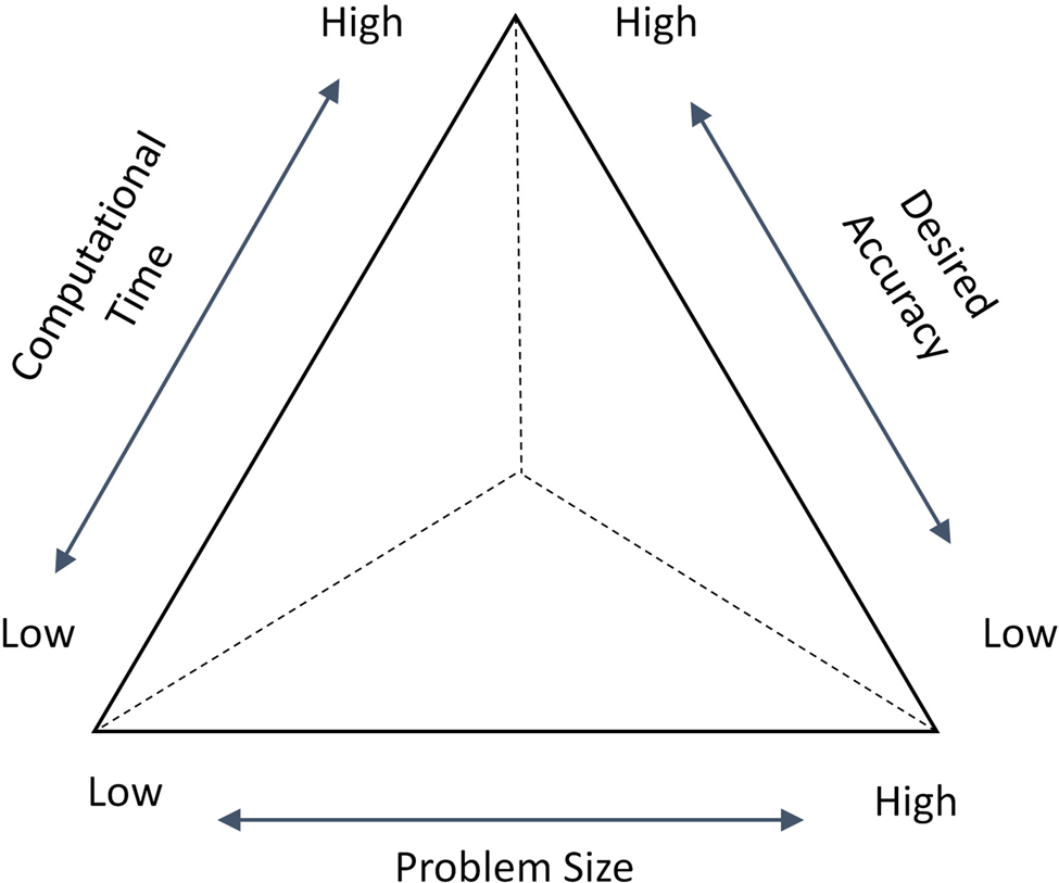
Fig. 1. Triangle showing the relationships among three design criteria (Alizadeh et al., Reference Alizadeh, Allen and Mistree2019).
Problem description
To test our hypothesis that an EoS is more accurate than those determined using individual RSM, KRG, RBF surrogates, we choose a hot rod rolling problem as an example. In this example problem, our interest is to accurately predict the microstructure of the final rod product using surrogate models such that the formation of banded microstructure (the microstructure with alternate layers of ferrite and pearlite occurring due to the presence of microsegregates, thereby affecting the mechanical properties) can be managed. The accuracy of the surrogate modeling process is hence important to properly estimate the final microstructure produced. As shown in Figure 2, in the hot rod rolling process problem that we are addressing, a billet of square cross-section having an initial austenitic microstructure is rolled using rollers and further cooled at the run-out table to change the shape, microstructure, and mechanical properties of the rod.

Fig. 2. Hot rod rolling process (Nellippallil et al., Reference Nellippallil, Rangaraj, Gautham, Singh, Allen and Mistree2017).
In this problem, we are only considering the phase transformation of austenite to the two phases, ferrite and pearlite. We assume in this problem that the phase transformation of austenite to ferrite and pearlite occurs only during the cooling stage after hot rolling. Two types of ferrite phases, namely allotriomorphic ferrite and Widmanstatten ferrite, are considered in this problem. A slow cooling rate favors the formation of banded ferrite/pearlite microstructure as there is enough time for carbon diffusion and ferrite (allotriomorphic ferrite mostly) nucleation.
Suppressing banding is possible via fasting cooling rate, but the elimination of microsegregates, the source for banding, is not possible. In addition to the cooling rate, the initial austenite grain size (AGS), percentages of carbon and manganese are important variables in the phase transformation process. For example, a small AGS facilitates the phase transformation to ferrite. A small AGS supports the increase of grain boundary area per volume available for nucleation resulting in more allotriomorphic ferrite nuclei and smaller ferrite grain sizes. This occurs at regions of low manganese concentrations. The rest of austenite transforms to pearlite phase. A high AGS, however, results in an increase in Widmanstatten ferrite. A banded microstructure of ferrite and pearlite formed due to the presence of microsegregates is shown in Figure 3.

Fig. 3. An example of a banded microstructure in 1020 steel consisting of ferrite (light) and pearlite (dark) (Jägle, Reference Jägle2007).
In prior studies, authors report the effects of banded microstructures on the mechanical properties of final products (see Spitzig, Reference Spitzig1983; Tomita, Reference Tomita1995; Krauss, Reference Krauss2003; Korda et al., Reference Korda, Mutoh, Miyashita, Sadasue and Mannan2006). Hence, it is critical to properly predict the microstructure after phase transformation to manage the banded microstructure such that the mechanical properties of the product can be controlled. The ferrite–pearlite banded microstructure is primarily caused due to microsegregates in the form of alloying elements of manganese, sulfur, etc., that are embedded into the steel during the solidification process after casting. The initial AGS, cooling rate, carbon concentration, and manganese concentration are selected in this study based on literature review as the major factors influencing the final microstructure phase formed after rolling and cooling. The program STRUCTURE developed by Jones and Bhadeshia (Reference Jones and Bhadeshia2017) is used as the simulation program to predict the microstructure phases. The other input fixed parameters for the simulation program like the austenite–ferrite interfacial energy, activation energy for atomic transfer, aspect ratio for nucleation of ferrite, fraction of effective boundary sites, total volume fractions of inclusions, nucleation factor for pearlite and aspect ratios of growing allotriomorphic ferrite, Widmanstatten ferrite, and pearlite are selected and defined based on the values reported by Jägle (Reference Jägle2007). The control factors thus considered in this work are described in Table 3. The output of the simulation includes volume fractions of pearlite and two types of ferrites, namely allotriomorphic ferrite and Widmanstätten ferrite for the different values of each of the four input variables. Therefore, the simulation addressed in this problem involves four input variables and three output variables.
Table 3. The design variables

A fractional factorial design of experiments (DOE) to generate response data sets is carried out by Nellippallil et al. (Reference Nellippallil, Rangaraj, Gautham, Singh, Allen and Mistree2018) using the simulation program, STRUCTURE developed by Jones and Bhadeshia (Reference Jones and Bhadeshia1997). Polynomial RSMs are fit for each of the responses. Nellippallil et al. explain how different values of the four input variables, cooling rate, carbon concentration, manganese concentration, and AGS affect the final microstructural phases (pearlite, allotriomorphic ferrite, and Widmanstätten ferrite) based on the polynomial RSM developed (Nellippallil et al., Reference Nellippallil, Rangaraj, Gautham, Singh, Allen and Mistree2018). Nellippallil et al. verify the model predictions by comparing them with experimentally measured data reported by Bodnar and Hansen (Reference Bodnar and Hansen1994). We use the fractional factorial DOE data set by Nellippallil et al. in this work. In Figure 4, we show the comparison of polynomial RSM predictions by Nellippallil et al. (Reference Nellippallil, Rangaraj, Gautham, Singh, Allen and Mistree2017) with the phase fractions reported in the literature by Bodnar and Hansen (Reference Bodnar and Hansen1994). We observe from Figure 4 that the model predictions lie in the vicinity of the straight line depicting the measured values.

Fig. 4. Comparison of polynomial RSM predictions (Nellippallil et al., Reference Nellippallil, Rangaraj, Gautham, Singh, Allen and Mistree2017).
Method
As shown in Figure 5, the procedure consists of several steps. The first step is to find some criteria to choose the most appropriate surrogate model. Based on a comprehensive critical literature review, a balanced triangle of three important characteristics of the experiment (accuracy, size, and time) are presented in Figure 1 (Alizadeh et al., Reference Alizadeh, Allen and Mistree2019). The second step is to build surrogate models, including RSM, KRG, RBF, and an ensemble of them. In this step, we compare the performance of these models for the hot rod rolling problem. In the third step, the outcome of the second step is summarized in a sort of database to be used in the future.

Fig. 5. Method for selecting the surrogate model based on time, size, and accuracy.
Surrogate modeling process
The method for selecting the surrogate model based on time, size, and accuracy are illustrated in Figure 5. After identifying the problem in the Problem description section, the next step is to generate sampling data. The DOE is used to obtain the sampling data over the desired range of input variables. In the second step, cross-validation (CV) is used to divide the design data into “training data” and “testing data” (Fig. 6). The “training data” is used to develop different surrogate models, and the “testing data” is used as unknown data to estimate the performance of different surrogate models. Next, different surrogate modeling methods are used to fit the training design data generated and develop a predictive model (in the Function fitting section). Finally, the surrogates are evaluated using the RMSE of the response deviation between the prediction data and the test data (in the Prediction metric: root-mean-square error section).
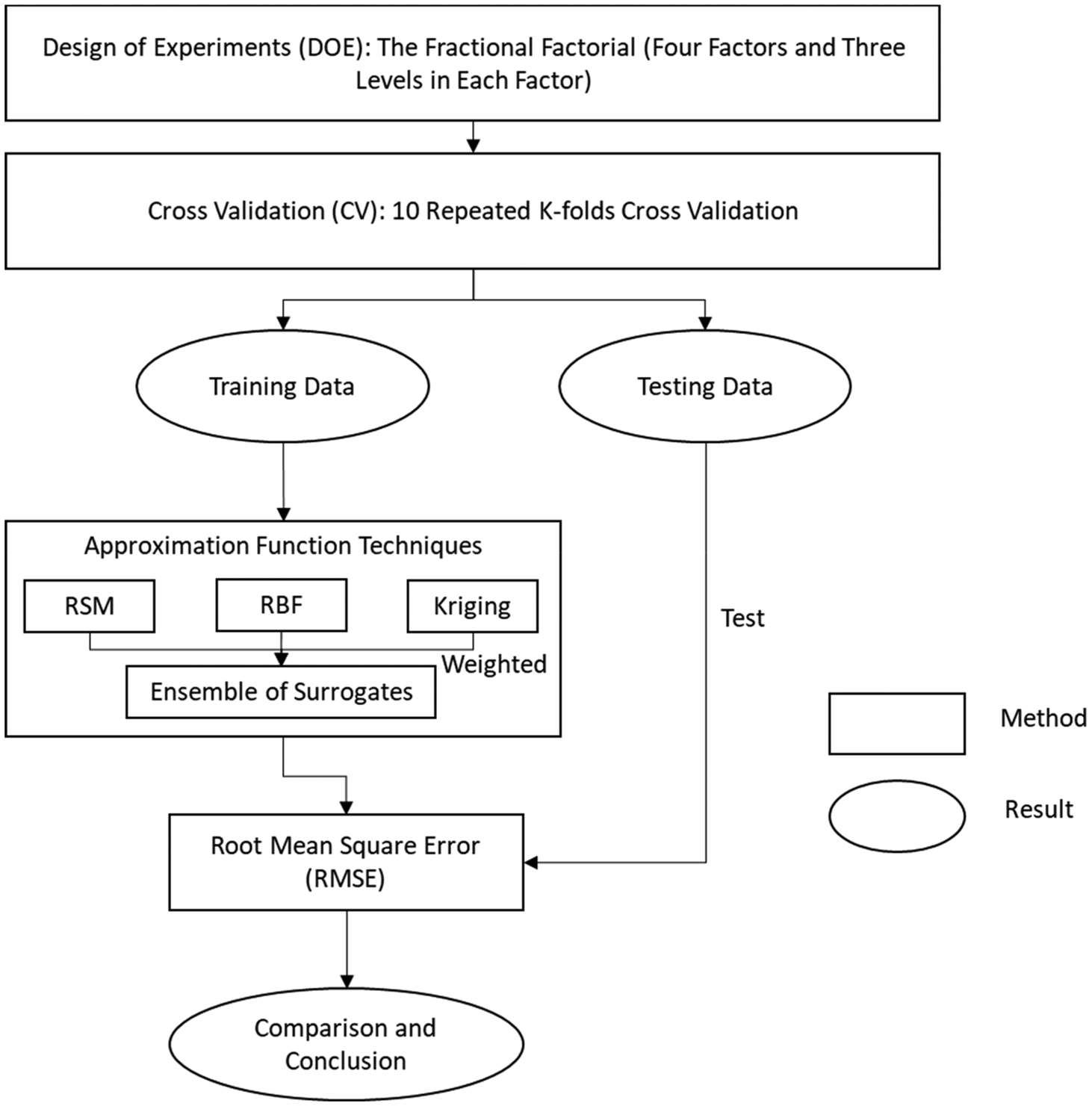
Fig. 6. The experimental procedure.
DOE and cross-validation
In this work, we use the data generated by Nellippallil et al. (Reference Nellippallil, Rangaraj, Gautham, Singh, Allen and Mistree2018) using a fractional factorial design (Montgomery, Reference Montgomery2017) to organize the experiments. Considering the trade-off between the cost of evaluation of the original simulation and the increase of fidelity associated with the increasing number of sampling data, three levels including the upper, lower, and middle points of the range in each factor are selected to manage the sampling process. The factors and factor levels are shown in Table 4.
Table 4. Factors and factor levels for DOE

Now, in order to estimate the performance of the predictive model, K-fold cross-validation is used. K−1 equally sized randomly selected subsamples are used as training data and the remaining single subsample is retained to test the model. The training process for each fold is repeated K−1 times, with each subsample being used exactly once as test data. Thus, all observations are fully used for both training and testing. We repeat the whole cross-validation process ten times, and the result is the average value of ten runs of cross-validation. In this way, the impact of noise can be minimized. The next step is to use the training data to construct surrogates, in this case, RSM, KRG, RBF, and an EoS and use the testing data for evaluation.
Function fitting
Several function approximation techniques are used as surrogates. Shyy et al. (Reference Shyy, Tucker and Vaidyanathan2001) used RSM and RBF to rocket engine design and compare the prediction of alternative models. It turns out surrogate models have good performance in prediction work. Zerpa et al. (Reference Zerpa, Queipo, Pintos and Salager2005) integrate RSM, KRG, and RBF as an ensemble of the surrogate model and apply it into an alkaline–surfactant–polymer flooding processes. Bellucci and Bauer (Reference Bellucci and Bauer2017) use RSM, KRG, and RBF to make robust parameter design. So, in this work, we choose RSM, KRG, and RBF, which are commonly used in the previous papers, and their combination as an ensemble of surrogate models to develop different prediction models.
Response surface method. The RSM is also known as the polynomial regression method which has the simplest of parameters (i.e., coefficients in a polynomial function) and is calculated using least squares regression (Razavi et al., Reference Razavi, Tolson and Burn2012). In this work, we use a second-order polynomial function as the surrogate model.
If x is an independent vector of factors, y is the vector of responses, the impact of x on y and their relationship can be illustrated as follows:
 $$ {{\hat {\bi y}}}({\bi x}) = \alpha _0 + \sum\limits_{i = 1}^n {\alpha _ix_i} + \sum\limits_{i = 1}^n {\alpha _{ii}x_i^2} + \sum {\sum\limits_{i \lt j} {\alpha _{ii}x_ix_j}}, $$
where α represents the coefficients of the polynomial function, and n is the number of independent factors.
Kriging. Kriging is a type of interpolating technique which is a polynomial model of an input vector of factors x, f(x), and localized deviation of x, g(x), as follows:
 $${{\hat {\bi y}}}({\bi x}) = f ({\bi x}) + g({\bi x}), $$
f(x) is the polynomial term, which is a global function over the entire input space (Razavi et al., Reference Razavi, Tolson and Burn2012). Usually, f(x) is a constant number or a linear polynomial function. And g(x) is a localized deviation function or can be called the basic function. In this article, the focus is on one type of KRG called Ordinary Kriging (Kleijnen, Reference Kleijnen2017).
 $$ { {\hat {\bi y}}}({\bi x}) = \mu + g({\bi x}), $$
where μ is an unknown constant, which represents the simulation output averaged over the experimental area, and g(x) is a zero-mean stochastic process.
Radial basis function. The RBF technique is based on a mathematical function and its value is calculated based on the distance the between origin and each point (Montgomery, Reference Montgomery2017). Alternatively, the distance between the center point and each point can be used as shown in the following equation:
 $$r_{i\comma \,j} = r\lpar {{\bi x}_{\bi i}\comma \,{\bi x}_{\bi j}} \rpar = \parallel \!\! {\bi x}_{\bi i}-{\bi x}_{\bi j} \! \! \parallel, $$
where r i,j denotes the Euclidean distance between two different sample points. Radial functions are employed to connect the distance r with the outputs, then the integration of these functions is used to estimate complicated mathematical functions. These functions are then used in constructing the surrogate models:
 $${\hat y}\lpar {{\bi x}_{{\rm new}}} \rpar = \sum\limits_{i = 1}^{M} {r_i Q \lpar \!\! \parallel\! \! {{\bi x}_{{\rm new}}-{\bi x}_{\bi i}} \! \! \parallel \! \! \rpar } {\bi }. $$
 The surrogate function  ${\hat y}\lpar {{\bi x}_{{\rm new}}} \rpar$ is an integration of M RBFs and each of them is linked to a distinct x i and has a weight of r i (Mirjalili, Reference Mirjalili and Mirjalili2019). In this work, the Gaussian function is selected as the RBF.
Ensemble of surrogates model. We use the weighted average model proposed by Goel et al. (Reference Goel, Haftka, Shyy and Queipo2006) to create the EoS. As we just use three individual surrogate models, the predicted response of the ensemble of surrogate model is
 $${\hat y}_{\rm EoS} = \sum\limits_i^{N_{\rm SM}} {w_i{{\hat y}}_i} = w_{\rm RSM}{\hat y}_{\rm RSM} + w_{\rm KRG}{\hat y}_{\rm KRG} + w_{\rm RBF}{\hat y}_{\rm RBF}, $$
where w i is the weight of each individual surrogate, and  ${\hat y}_i$ is the predicted response of the ith individual surrogate.
For the selection of weights, a strategy which is based on generalized mean square cross-validation error (GMS error) is proposed in Goel et al. (Reference Goel, Haftka, Shyy and Queipo2006).
 $$w_i{^\ast} = \lpar {E_i + \alpha E_{\rm avg}} \rpar ^\beta\comma \, \quad w_i = \frac{w_i^{\ast}}{\sum\limits_i {w_i^{\ast}}},$$
 $$E_{\rm avg} = \frac{\mathop \sum \nolimits_i^{N_{\rm SM}} E_i}{N_{\rm SM}}, $$
where E i denotes the GMS error, N SM is the number of sample points, and two constraints, α, β are chosen to be α = 0.05 and β = −1, respectively (Samad et al., Reference Samad, Kim, Goel, Haftka and Shyy2006).
Prediction metric: root-mean-square error
In evaluating the process, the actual objective function value for the testing data is known and regarded as the target value. This value is then used to calculate the error at all testing points. The RMSE is used as the prediction metric to assess the accuracy of each prediction model generated by different surrogates. The definition of RMSE is
 $${\rm RMSE} = \sqrt {{{\sum\nolimits_{i = 1}^{N_{{\rm test}}} {{\lpar {y_i-{{\hat y}}_i} \rpar }^2}} \over {N_{{\rm test}}}}}, $$
where N test represents the number of testing points, y i, and  ${\hat y}_i$ are the actual response and the predicted value of the response from a surrogate. The lower the RMSE, the greater the accuracy of the surrogate model, and vice versa.
Results and discussion
Comparison between ensembles of surrogates and individual surrogates
Appendix A contains the sample points for the three objectives, allotriomorphic ferrite (Y1), Widmanstätten ferrite (Y2), and pearlite (Y3). In order to generate test data to validate the performance of these surrogate models, we repeat a ninefold cross-validation process ten times. In each run, all data sets are randomly partitioned into nine subsamples (groups). Of the nine subsamples, one subsample is used as the testing data set and the remaining eight subsamples are used to train the model. Through nine repetitions, all observations are involved in training and testing. Three outputs are allotriomorphic ferrite (Y1), Widmanstätten ferrite (Y2), and pearlite (Y3) of steel.
In two upper plots of Figure 7, we indicate the RMSE for the prediction of output Y1 (allotriomorphic ferrite) and output Y2 (Widmanstätten ferrite), respectively. In the two lower plots of Figure 7, we represent the RMSE of output Y3 (pearlite). The difference is that in the left one, we show the errors of four surrogates, in the right one, we show the expanded version for the EoS, KRG, and RSMs.

Fig. 7. RMSE in the prediction of surrogates in ten runs.
The experimental results for three outputs from the hot rod rolling problem with RSM, KRG, RBF, and an EoS are shown in Figure 7. The result shows that RBF gives the highest RMS error for all three objectives, especially for output Y3 (Pearlite), the error of the RBF is almost five times larger than other three surrogates, which means RBF has the lowest accuracy in predicting all three objectives. Also, the difference between the EoS, KRG, and RSM is minimal, but the EoS shows subtle advantages in accuracy.
As for the quantitative validation of the surrogates, a statistical analysis of RMS errors of surrogate predictions for ten runs in the design space is shown in Table 5. EoS has the best accuracy except for Y2 (Widmanstätten ferrite), and RBF is the least accurate. For Y2, EoS has the second-highest accuracy, which is second to RSM and the difference between these two is very small  $(0.0478-0.0447)/0.0478\approx 6.5{\rm \%.}$ This indicates that an EoS has the most appropriate performance for the hot rod rolling problem because of its accuracy and relatively insensitive predictions to the number of data points for all three objectives and therefore ensembles of surrogates are more robust.
Table 5. Statistical analysis of RMSE value by various surrogates in ten runs

The bold numbers are the lowest root mean square errors.
Trade-offs among accuracy, size, and time
To find a relationship among the size, accuracy, and computation time of surrogates for the hot rod rolling problem, we change the size of the problem in terms of the number of training data which are used to train the prediction model. As the sample data has 27 points and the K-fold cross-validation is used to generate the training data, we increase training data by the way of decreasing the fold value. The relationship between the fold number and the test data can be expressed as a function:
 $$N_{{\rm test}} = 27-\frac{27}{N_{{\rm fold}}}, $$
where N test is the number of test data, N fold is the fold number. Thus, when the fold value decreases from ninefolds to twofolds, the training data will be reduced from 24 to 14. In order to make a fair comparison between four different surrogates, the model training process is organized with the same training data. The comparison between these four surrogates in three outputs of the hot rod rolling problem is shown in Figure 8.

Fig. 8. RMS errors in the prediction of surrogates with different folds of data from 9 to 2.
With the upper two plots in Figure 8, we indicate the RMS errors of predicting Y1 (allotriomorphic ferrite) and output Y2 (Widmanstätten ferrite). With the lower two plots of Figure 8, we represent the RMS errors of output Y3 (pearlite). The difference is that with the left one, we show the errors of four surrogate and with the right one, we only show three (except RBF). From Figure 8, for each surrogate model, the RMS error gradually increases as the amount of training data decreases, therefore accuracy has a negative correlation with the number of samples used in the training data, and this trend is in-line with our intuition. In addition, it is interesting that the error curves of each surrogate all have a smooth change from the ninefold to fourfold training data but abruptly increase at the three- and twofold data, especially the RSM and RBF. That is because, with small numbers of training data (two- and threefold), surrogate models are more prone to have low fidelity compared to the associated physical problem. As for the comparison between these four surrogates, EoS, KRG, and RMS have relatively lower RMS error and higher accuracy than RBF for all folds. EoS and KRG generally show very robust behavior, and RSM also shows a robust behavior until two- and threefold data are used, where there is a sharp surge in error, and the RSM's accuracy goes down immediately.
The program run time is the computational time required by Python codes in a Lenovo computer i7-4720HQ 8G 128G SSD+1T GTX960M.
As can be seen in Table 6, RBF has the lowest program run time among the four surrogates. However, from a practical perspective, the time should include not only the program run time which is consumed to construct the surrogate model but also the simulation time used for sampling. So, in this work, the time is defined as follows.
 $$T = T_{\rm pm} + T_{\rm sm}, $$
where T pm is the program run time, and T sm is the simulation time.
Table 6. Program run time to compute values for four surrogates from nine- to twofold training data for output Y1

The bold numbers are the lowest root mean square errors.
In the hot rod rolling problem, the average sampling time for generating each data point in the simulation is about 3.5 h (12,600 s), which is at least two orders of magnitude larger than the program run time (the longest one is about 150 s) for all four surrogates. So, the program run time can be ignored in Eq. (10), and the time we mention in the following discussion is the equivalent of the sampling time, as shown in the following:
 $$T\approx T_{{\rm sample}} = 3.5\, {\rm h} \times N_{{\rm sample}}, $$
where the N sample is the number of sample points. Therefore, the time is proportional to the number of sample points. In order to generate selection rules, a detailed comparison of results among the different surrogate models for each output is shown in the following three sections.
Results for output Y1 (allotriomorphic ferrite)
The RMS errors, namely the accuracy, for each surrogate for different numbers of design data from nine- to twofolds are shown in Figure 8. Ensembles of surrogates have relatively lower RMS errors and therefore higher accuracy than three individual surrogates for the nine-, eight-, seven-, six-, five-, and fourfold data. In addition, ensembles of surrogates in two- and threefold data have almost equal accuracy (The difference is about 0.001.) and two- and threefold KRG have much higher accuracy than RSM and RBF. Both KRG and an EoS have higher accuracy than RBF in all K-fold cross-validation methods. Also, they have higher accuracy even when we use twofold cross-validation for them and ninefold cross-validation for RBF. So, RBF is not a good choice regarding the accuracy and size measures.
In Table 7, we bold the lowest values of error for each number of folds in bold. It shows that the RMS error gradually decreases with decreasing training data for each surrogate, which means that the accuracy is negatively correlated with the amount of training data, and this trend is in-line with our intuition.
Table 7. RMS errors generated by four different surrogates from nine- to twofold training data for output Y1

The bold numbers are the lowest values of error for each number of folds.
In addition, an EoS has much greater accuracy than the other three individual surrogates trained for ninefold data even when we use eight-, seven-, six-, five-, and fourfolds instead of ninefold data. So, an EoS gives the most accurate predictions and needs the lowest time to obtain the prediction for allotriomorphic ferrite when we use nine- to fourfold training data. Also, RBF is not a good choice because time, accuracy, and size measures for ninefold cross-validation for RBF is not greater than the twofold cross-validation for the ensembles of surrogates and KRG. As for the comparison between RSM and EoS, EoS has greater accuracy than RSM in four- to ninefold cross-validation. When we use threefold data to train the EoS, we obtain higher accuracy than when we use ninefold of data to train RSM. Also, we obtain higher accuracy by using five- to eightfold of RSM rather than using twofold of data to train the EoS, while RSMs trained with two- to fourfold of data have lower accuracy than EoS trained with twofold data.
Based on this analysis, some recommendations for time and size of the data set along with the accuracy of output 1 (Y1) can be developed. If we consider the EoS individually, by using twofold instead of ninefold, accuracy will increase about  $(0.07-0.035)/0.07 = 50\%$. On the other hand, by using twofold instead of ninefold, we need (27–27/2 = 13)*3.5 = 45.5 h instead of 27*3.5 = 94.5 h, and so, there are a savings of 35 h. As for the comparison between ensembles of surrogates and individual surrogates, ensembles of surrogates are the recommended because of their higher accuracy and low time-consumption for four- to ninefold (19–24) training data, whereas RBF is always the worst choice.
Results for output Y2 (Widmanstätten ferrite)
For Widmanstätten ferrite, the EoS has relatively lower RMS errors, and so, higher accuracy than KRG, and RBF even when we use nine-, eight-, seven-, six-, five-, four-, three-, and twofolds of the data. Although RSM has a relatively higher accuracy for nine-, eight-, seven-, six-, and fivefolds of data, again it has lower accuracy in two- and threefolds in comparison to the EoS. RBF also again has relatively low accuracy in comparison to other surrogate modeling methods. KRG also has relatively less accuracy for five- to ninefolds. RSM and has only greater accuracy than RSM in two- to fourfolds. Interestingly, RSM with fewer data points, including five-, six-, seven-, and eightfolds has better accuracy than ninefold KRG.
From the analysis in Table 8, some recommendations considering the time and size of the data set along with the accuracy for Widmanstätten ferrite (Y2) are developed. Entries in bold show the lowest values of error for each number of folds. If we consider the EoS by itself, by using twofold instead of ninefold, accuracy will increase about  $(0.08-0.035)/0.08 = 0.43\%$. On the other hand, by using twofold instead of ninefold data, we need 45.5 h instead of 94.5 h, and so, we can save 35 h. Also, to compare ensembles of surrogates with other single surrogates, by using a fourfold EoS, we need 70.87 h instead of 94.5 h when we choose to use ninefold RSM, and so, we can save 23.63 h (23.63 h faster surrogate) and have
  $(0.055-0.04)/0.055 = 27\%$ less accuracy.
Table 8. RMS errors generated by four different surrogates from nine- to twofold training data for output Y2

The bold numbers are the lowest values of error for each number of folds.
Results for output Y3 (pearlite)
As shown in Table 9, there is a slight difference between the accuracy of EoS, KRG, and RSM except for two- and threefold RSM which has much lower accuracy. On the other hand, there is a huge gap among these three surrogates and RBF, which has very low accuracy and can hardly be compared with others. If we consider surrogates individually, there is almost no difference among using four-, five-, six-, eight-, ninefolds of KRG and EoS. Therefore, it is possible to save 23.63 h by using fourfold KRG or and an EoS instead of ninefold KRG or and an EoS. Also, for RSM, there is a very slight difference between using fourfold instead of ninefold. While using threefold RSM, the accuracy will reduce  $(0.035-0.03)/0.035 = 14\%$, but the process will be much faster. In other words, by using threefold instead of ninefold, 63 h instead of 94.5 h are needed, which can save 31.5 h. It also means that we can use only 9 data points instead of 27 data points which saves 67% of the simulation time which we need to spend to generate the simulation data.
Table 9. RMS errors generated by four different surrogates from nine- to twofold training data for output Y3

The bold numbers are the lowest root mean square errors.
The summary of the results is given in Table 10. The highlighted values denote to the lowest RMS error obtained from the corresponding surrogate model. As illustrated in Table 10, for the first response variable, Y1 (allotriomorphic ferrite), in four- to ninefolds of data, an EoS has lower RMSE than individual surrogates and only for two- and threefolds of data, KRG has lower RMSE than others. Also, for the second response variable, Y2 (Widmanstätten ferrite), in two- to fourfolds of data, EoS has lower RMSE than other surrogates. Finally, for the third response variable, Y3 (pearlite), in four- to ninefolds of data, EoS has lower RMSE than other surrogates
Table 10. RMS errors generated by four surrogates from nine- to twofold training data for output Y1, Y2, and Y3

Bold values mentioned the highlighted values denote to the lowest RMS error obtained from the corresponding Surrogate model.
In comparison to some other studies, such as Viana et al. (Reference Viana, Haftka and Watson2013), Chaudhuri and Haftka (Reference Chaudhuri and Haftka2014), Badhurshah and Samad (Reference Badhurshah and Samad2015), and Bhattacharjee et al. (Reference Bhattacharjee, Singh and Tapabrata2018) in ensemble surrogates related issues, there is a big difference in the method. Authors in these papers applied multiple surrogate methods for multiobjective optimization, while in this paper, we used an EoS for prediction. Also, Goel et al. (Reference Goel, Haftka, Shyy and Queipo2007) and Bishop (Reference Bishop1995) create a WAS by estimating the covariance between surrogates from residuals at test or training data sets and using the PWS, while we create the weights based on cross-validation errors. Basudhar (Reference Basudhar2012), Viana et al. (Reference Viana, Haftka and Watson2013), Bhattacharjee et al. (Reference Bhattacharjee, Singh, Ray and Branke2016), and Ezhilsabareesh et al. (Reference Ezhilsabareesh, Rhee and Samad2018) used an EoS in a relatively high number of data, while we use an EoS in small data size.
In addition, the ensembles created by Chaudhuri and Haftka (Reference Chaudhuri and Haftka2014), Wang et al. (Reference Wang, Ye, Li and Li2016), Bhattacharjee et al. (Reference Bhattacharjee, Singh and Tapabrata2018), Lv et al. (Reference Lv, Zhao, Wang and Liu2018), Song et al. (Reference Song, Lv, Li, Sun and Zhang2018), and Yin et al. (Reference Yin, Fang, Wen, Gutowski and Xiao2018) are more time consuming than each individual surrogate they used to create the ensemble. Whereas, we create ensembles which are less time consuming than individual surrogates and have less inconsistency.
In order to give specific guidance for surrogate selection, a rule-based template is given in Table 11. For the hot rod rolling problem, three tables as decision trees corresponding to the three outputs are developed to manage the selection among the four types of surrogate. As we have three characteristics for the problem, accuracy, size, and time, and time is directly proportional to size, the selection of appropriate surrogates can be based on accuracy and size. In this work, accuracy is used as the criterion for the first selection, and size is the criterion for the second selection. Specific guidance for the selection of surrogate models for output Y1 is shown in Table 11 as an example. There is no surrogate model which gives us RMSE < 0.03, while EoS can be used if accuracy 0.03 ≤ RMSE < 0.05 is needed, and here, EoS is the choice based on the first selection criteria (RMSE). Also, for the second selection criteria (time), five- to eightfold can be chosen when we need to spend no more than 84 s to run the code for the surrogate model.
Table 11. Specific guidance for the selection of surrogate models for output Y1 (allotriomorphic ferrite)

Closing remarks
Based on the published literature, creating an EoS using cross-validation errors results is higher accurate, but it is more computationally intensive than using individual surrogates. Our contribution in this paper is to propose a method to build an EoS that is both accurate and less computationally expensive. The novelty in this paper is to propose a method based on cross-validation to find an EoS which is created by the least possible number of data points. The resulting ensemble surrogate has higher accuracy than each individual surrogate and is less computationally intensive. To achieve this ensemble surrogate, we compare it with individual surrogate models based on computation time, size, and desired accuracy. For this purpose, we use RMSE as the accuracy measure, time of simulation as the computation performance measure, and the number of data points as the dimension measure. In summary, we find that (1) it is effective to use cross-validation to study the impact of the size of the sample data set; (2) the highest accuracy with least required data and less computation time is achievable using the right number of samples; and (3) an example of surrogates is relatively insensitive to the size of the sample data or number of data points. We create rule-based guidance for selection of surrogate models for one of the response variables in Table 11. Creating rule-based templates for each response variable and putting them together into a knowledge-based platform and ontology is possible future research. As another possible research direction, these knowledge-based platforms and ontology can be used in automating the surrogate modeling process.
This paper is based on several assumptions: (1) hot rod rolling process is a single independent engineering process and (2) we are able to create a surrogate model for hot rod rolling considering it as an independent engineering process. Removing these assumptions and considering the casting and reheating as preprocesses along with cooling and forging as post processes is another possible future research direction that we can take. Furthermore, we create rule-based guidance for selection of surrogate models for one of the response variables in Table 11. Creating rule-based templates for each and every response variable and putting them together into a knowledge-based platform and ontology is possible future research. As another possible research direction, these knowledge-based platforms and ontology can be used in automating the surrogate modeling process.
Acknowledgments
Reza Alizadeh, Anand Balu Nellippallil, Janet K. Allen, and Farrokh Mistree acknowledge financial support from the John and Mary Moore Chair and the L.A. Comp Chair at the University of Oklahoma. Guoxin Wang, Liangyue Jia, and Jia Hao also acknowledge financial support from the National Ministries of China (JCKY2016602B007). This paper is an outcome of the International Systems Realization Partnership between the Institute for Industrial Engineering at The Beijing Institute of Technology, The Systems Realization Laboratory at The University of Oklahoma and the Design Engineering Laboratory at Purdue.
Appendix A Sample data for the hot rod rolling problem
The sample points for the three objectives, allotriomorphic ferrite (Y1), Widmanstätten ferrite (Y2), and pearlite (Y3), are summarized in this section. To generate test data to validate the performance of these surrogate models, we repeat a ninefold cross-validation process ten times. In each run, all data sets are randomly partitioned into nine subsamples (groups). Of the nine subsamples, one subsample is used as the testing data set and the remaining eight subsamples are used to train the model. Through nine repetitions, all observations are involved in training and testing. Three output variables, namely allotriomorphic ferrite (Y1), Widmanstätten ferrite (Y2), and pearlite (Y3) of steel are predicted based on values of five input variables, namely carbon concentration rate, manganese concentration rate, grain size, cooling rate, and final temperature. The prediction results are shown in Table 12.
Table 12. Values for input and output variables

The bold numbers are the lowest root mean square errors.
Reza Alizadeh received his BSc in Industrial Engineering from the Urmia University of Technology in 2011. He also received his MSc in Technology Foresight from the Amirkabir University of Technology in 2013. He is currently a PhD candidate in Industrial and Systems Engineering at the University of Oklahoma, USA. His current research interests include simulation-based design, surrogate modeling, network analysis, data analytics, decision-making under uncertainty, and cloud-based design.
Liang Jia received the MS degree in Mechanical Engineering from the Beijing Institute of Technology, China, in 2018, where he is currently pursuing the PhD degree. His research interests include intelligent manufacturing systems and intelligent design.
Anand Balu Nellippallil received his BTech, in Production Engineering from the University of Calicut in 2012. He also received his MTech, in Materials Science and Engineering from the Indian Institute of Technology Bhubaneswar in 2014. He also received his PhD degree in Aerospace and Mechanical Engineering from the University of Oklahoma, USA, in 2018. He is currently a Research Engineer II at the Center for Advanced Vehicular Systems, Mississippi State University. His current research interests include “integrated realization of engineered materials, products and associated manufacturing processes” with emphasis on the following research thrusts: simulation-based design, robust design, design decision-making under uncertainty, and cloud-based design decision support.
Guoxin Wang received the BS degree from Lanzhou Jiaotong University in 2001, the MS degree from Lanzhou Jiaotong University in 2004, and the PhD degree from the Beijing Institute of Technology, China, in 2007. He was a Visiting Scholar at the University of Oklahoma, USA, from 2014 to 2015. He is currently an Associate Professor with the Beijing Institute of Technology. His current research interests include reconfigurable manufacturing systems, intelligent design, and knowledge engineering.
Jia Hao received the MS and PhD degrees in Mechanical Engineering from the Beijing Institute of Technology, China, in 2010 and 2014, respectively. He is currently an Assistant Professor with the Beijing Institute of Technology. His current research interests include intelligent design, computational creativity, and related area.
Janet K. Allen received the SB degree from MIT in 1967, and the PhD degree from the University of California, Berkeley, in 1973. She was a Senior Research Scientist at the George W. Woodruff School of Mechanical Engineering between 1992 and 2009. She is currently John and Mary Moore Chair and professor at the University of Oklahoma, USA. Her current research interests include simulation-based design of engineering systems, managing uncertainty in design, sustainability, and design pedagogy.
Farrokh Mistree received the BS degree from IIT Kharagpur in 1967, the MS degree and the PhD degree from the University of California, Berkeley, in 1970 and 1974, respectively. He was the Director of the School of Aerospace and Mechanical Engineering between 2009 and 2013. He is currently the L.A. Comp Chair and Professor at the University of Oklahoma, USA, from 2014 to 2015. Before joining the University of Oklahoma, he was a professor at Georgia Institute of Technology and the Associate Chair of the Woodruff School of Mechanical Engineering. His current research interests include knowledge-based realization and management of complex engineering systems.


