


Introduction
Depression is one of the most common mental disorders affecting older people, which often coexists with other medical illnesses and physical disabilities (Richard et al., Reference Richard, Birrer, Sathya and Vemuri2004). People with diagnosed clinical depression or depressive symptomatology are at higher risk of mortality (Bruce and Leaf, Reference Bruce and Leaf1989; Penninx et al., Reference Penninx, Geerlings, Deeg, van Eijk, van Tilburg and Beekman1999; Pulska et al., Reference Pulska, Pahkala, Laippala and Kivelä1999). The evidence of higher prevalence of depression among women than among men is one of the most widely documented findings, in both population-based and clinical studies (Dennerstein et al., Reference Dennerstein, Astbury and Morse1993; Kessler, Reference Kessler and Frank2000, Reference Kessler2003). The gender differences in depression have been found to persist also during later life (Beekman et al., Reference Beekman, Copeland and Prince1999; Cole and Dendukuri, Reference Cole and Dendukuri2003; Pagán-Rodríguez and Pérez, Reference Pagán-Rodríguez and Pérez2012).
Later-life depression is characterised by a large heterogeneity in symptoms and significantly decreases quality of life of the older population. Nevertheless, there is not a general agreement in the scientific literature on what constitutes clinically significant depression, nor on how to profile depressive and emotional symptoms (Blazer, Reference Blazer2003).
The identification of substantial and meaningful sub-groups of depressive symptom profiles among the old population has important implications for research, public health policies and clinical practice.
On the one hand, the public health burden of depressive symptoms in older adults is expected to increase rapidly, given the large proportion of people in this group. Not surprisingly, the theme of the 2017 World Health Day campaign was depression.
On the other hand, as stated by Hybels et al.:
the structure of depressive symptoms in older adults may differ from that observed in younger adults since depression in older adults like other psychiatric syndromes can be more heterogeneous and affected by variables such as age of onset, number of lifetime episodes, and particularly, comorbidity, which can contribute to, be associated with, or result from psychopathology. Work is needed to identify symptom profiles in both community and clinical populations of older adults. (Hybels et al., Reference Hybels, Blazer, Pieper, Landerman and Steffens2009: 389)
First, depression in older adults may be more difficult to recognise than in the younger population. As underlined by Birrer and Vemuri (Reference Birrer and Vemuri2004), older patients with depression do not usually report depressed moods, in favour of less-specific symptoms such as insomnia, anorexia and fatigue; then, less-severe depression is not taken seriously because it is perceived as a normal part of the ageing process or the life stress.
Minor depression, which is a clinically significant depressive disorder that, however, does not fulfil the criteria for the diagnosis of major depression, such as duration and the number of symptoms (American Psychiatric Association, 1994), is more common among old patients than major depression (Beekman et al., Reference Beekman, Copeland and Prince1999). People with minor depression may often develop major depression within two years and are more likely to have a concomitant anxiety disorder (Birrer and Vemuri, Reference Birrer and Vemuri2004).
Yet, in older people depression may be confused with dementia or other brain disorders because these conditions share some of the same features (Boswell and Stoudemire, Reference Boswell and Stoudemire1996). Indeed, unlike younger persons with depression, old individuals with depression usually have a medical comorbidity, such as vascular diseases, diabetes, cancer, arthritis and so on (Sheikh et al., Reference Sheikh, Cassidy, Murali Doraiswamy, Salomon, Hornig, Holland, Mandel, Clary and Burt2004), and higher rates of cognitive impairment (Jones and Reifler, Reference Jones and Reifler1994). A personal and/or family history of depression increases the risk of developing depression in late life. Moreover, stressful events that frequently occur in later life, such as the death of a loved person or the loss of a job through retirement, may trigger depression (American Psychiatric Association, 1994).
Depression may be treated in an old population combining pharmacotherapy and psychotherapy, although evidence suggests that older patients with depression benefit most from aggressive and persistent treatment (Alexopoulos et al., Reference Alexopoulos, Katz, Reynolds, Carpenter, Docherty and Ross2001).
Several screening tools for depressive symptoms are used in clinical and non-clinical settings. These can be divided into two broader sets of instruments: the first, designed to collect information on symptoms, conditions or signs (in other words diagnostic criteria) that best reflect diagnoses of mental disorders. Of this type are the Diagnostic Interview Schedule (Robins et al., Reference Robins, Helzer, Croughan and Ratcliff1981) that assesses disorders using the definitions and criteria of the Diagnostic and Statistical Manual of Mental Disorders, 3rd Edn (DSM-III; American Psychiatric Association, 1980), the Composite International Diagnostic Interview (CIDI) (Robins et al., Reference Robins, Wing, Wittchen, Helzer, Babor, Burke, Farmer, Jablenski, Pickens, Regier, Sartorius and Towle1988), designed for assessing disorders based on the definitions and criteria of the Diagnostic and Statistical Manual of Mental Disorders, 3rd Edn Revised (DSM-III-R; American Psychiatric Association, 1987), CIDI extensions like the World Mental Health CIDI (Kessler and Üstün, Reference Kessler and Üstün2004) or the Structured Clinical Interview for DSM (SCID) (Spitzer et al., Reference Spitzer, Williams, Gibbon and First1992) and its subsequent revisions. While the Diagnostic Interview Schedule diagnoses are exclusively based on the definitions and criteria of the DSM, CIDI is also based on the World Health Organization International Classification of Disease. The second set of instruments are designed to measure more generic factors (i.e. psychological distress), collecting the presence or the absence of certain symptoms or emotional disorders, such as the Centre for Epidemiologic Study Depression Scale (CESD) (Radloff, Reference Radloff1977), the Beck Depression Inventory (Beck et al., Reference Beck, Steer and Garbin1988) and the EURO-D (Prince et al., Reference Prince, Reischies, Beekman, Fuhrer, Jonker, Kivelä, Lawlor, Lobo, Magnusson, Fichter, van Oyen, Roelands, Skoog, Turrina and Copeland1999b) scales. Usually, this kind of instrument provides a mental health score and cut-off points to be used to classify individuals in having (or not) depression or mental health disorders.
The EURO-D scale
The EURO-D is a depression scale that was developed and validated by the EURODEP Concerted Action Programme. The scale includes 12 items: depression, pessimism, wishing death, guilt, sleep, interest, irritability, appetite, fatigue, concentration, enjoyment and tearfulness (Prince et al., Reference Prince, Reischies, Beekman, Fuhrer, Jonker, Kivelä, Lawlor, Lobo, Magnusson, Fichter, van Oyen, Roelands, Skoog, Turrina and Copeland1999b). This scale is the result of the harmonisation of five depression measures, three interviewer-administered scales that generate clinical diagnoses (Geriatric Mental State-AGECAT, SHORT-CARE and Comprehensive Psychopathological Rating scale) and two self-reported depression symptom scales (CESD and Zung Self-rating Depression scale). EURO-D is a symptom-oriented scale, meaning that it identifies the presence (or not) of some depressive or emotional manifestations: its score ranges from 0 (the lowest level of depression) to 12 (the highest level), but it does not provide diagnoses of any mental disorders. The complete list of the EURO-D questions is reported in Table A1 in the online supplementary material.
Construct validity of this scale was supported by Larraga et al. (Reference Larraga, Saz, Dewey, Marcos and Lobo2006), Ploubidis and Grundy (Reference Ploubidis and Grundy2009) and, with some limitations, Brailean et al. (Reference Brailean, Guerra, Chua, Prince and Prina2015). Prince et al. (Reference Prince, Beekman, Deeg, Fuhrer, Kivelä, Lawlor, Lobo, Magnusson, Meller, van Oyen, Reischies, Roelands, Skoog, Turrina and Copeland1999a) showed that the EURO-D scale could be reduced into two factors, Affective Suffering and Motivation. Brailean et al. (Reference Brailean, Guerra, Chua, Prince and Prina2015) and Guerra et al. (Reference Guerra, Ferri, Llibre, Prina and Prince2015) found evidence on the validity of this scale with the two-dimensional structure across different populations. Overall, the Affective Suffering factor is characterised by very good cross-cultural measurement properties, while the Motivation factor shows heterogeneity in factor loading patterns and item calibrations across countries (Castro-Costa et al., Reference Castro-Costa, Dewey, Stewart, Banerjee, Huppert, Mendonca-Lima, Bula, Reisches, Wancata, Ritchie, Tsolaki, Mateos and Prince2008; Prince, Reference Prince, Patel, Minas, Cohen and Prince2013; Portellano-Ortiz et al., Reference Portellano-Ortiz, Garre-Olmo, Calvó-Perxas and Conde-Sala2018). There is strong support for applying in the empirical analysis both the full 12-item EURO-D scale and the Affective Suffering factor score derived from it, while the use of the Motivation factor in cross-cultural studies is suggested with some caution (Prince, Reference Prince, Patel, Minas, Cohen and Prince2013).
Dewey and Prince (Reference Dewey, Prince, Börsch-Supan, Brugiavini, Jürges, Mackenbach, Siegrist and Weber2005) defined clinically significant depression with a EURO-D score greater than 3. This cut-off point was validated in the EURODEP study, across the continent and against a variety of clinically relevant indicators (people with scoring above this level would be likely to be diagnosed as suffering from a depressive disorder, for which therapeutic intervention would be indicated). However, several studies have shown that a higher optimal cut-off point (4, 5 or even above) should be required in order to detect probable depression individuals (Castro-Costa et al., Reference Castro-Costa, Dewey, Stewart, Banerjee, Huppert, Mendonca-Lima, Bula, Reisches, Wancata, Ritchie, Tsolaki, Mateos and Prince2007; Jirapramukpitak et al., Reference Jirapramukpitak, Darawuttimaprakorn, Punpuing and Abas2009; Guerra et al., Reference Guerra, Ferri, Llibre, Prina and Prince2015).
Aims and hypotheses
Although widely used, a cut-off to identify people at risk of depression does not discriminate among depression sub-types nor does it allow a distinction to be made between mild and severe depression. As a result, depression may be under- or over-diagnosed (according to the value chosen as cut-off). Nevertheless, as previously described, older people may differentiate from others for the combinations of symptoms that characterise their mental disorders.
Therefore, the hypothesis underlying this work is that a more accurate classification (according to the number and type of the reported items) of the older individuals than the simple dichotomisation ‘depressed’ versus ‘non-depressed’ may be more helpful to researchers, clinicians and clinical investigators. The main objective of this work is to investigate the usefulness of an alternative approach, based on two model-driven solutions, for analysing data collected by the EURO-D scale. We want to identify meaningful sub-groups of depressive symptom profiles among a population sample of older individuals.
Data and method
The sample
This study is based on data from the sixth wave of the Survey of Health, Ageing and Retirement in Europe (SHARE), collected in 2015 (Börsch-Supan, Reference Börsch-Supan2017) (doi:https://doi.org/10.6103/SHARE.w6.600). For methodological details, see Börsch-Supan et al. (Reference Börsch-Supan, Brandt, Hunkler, Kneip, Korbmacher, Malter, Schaan, Stuck and Zuber2013) and Malter and Börsch-Supan (Reference Malter and Börsch-Supan2017).
SHARE is a panel survey that collects detailed cross-national information on health, socio-economic status, and social and family networks of citizens aged 50 and over from a large set of European countries, ranging from the Scandinavian and Baltic area to Mediterranean nations.
The analysed sample is composed of 64,716 individuals (who answered all items of the EURO-D scale), living in 18 countries (Austria, Belgium, Croatia, Czech Republic, Denmark, Estonia, France, Germany, Greece, Italy, Israel, Luxembourg, Poland, Portugal, Slovenia, Spain, Sweden and Switzerland). Sample size ranges from more than 5,000 observations in Belgium, Estonia, Italy and Spain to less than 2,000 in Israel, Luxembourg, Poland and Portugal.
In order to maximise the large sample size, we analysed the pooled data-set rather than by country. The EURO-D scale was specifically developed as a harmonised instrument across European countries (Prince et al., Reference Prince, Reischies, Beekman, Fuhrer, Jonker, Kivelä, Lawlor, Lobo, Magnusson, Fichter, van Oyen, Roelands, Skoog, Turrina and Copeland1999b). As a consequence, from its initiation each SHARE country has supported high-quality translation procedures (Harkness, Reference Harkness, Börsch-Supan and Jürges2005), in order to guarantee cross-country homogeneity in understanding the meaning of every question by respondents.
The statistical methods
Our approach is based on two different statistical solutions – Latent Class (LC) analysis and Factor Analysis (FA) – to classify individuals with different patterns of depressive disorders. Specifically, in the LC analysis the probability of belonging to each class is calculated for every individual. However, the LC solution usually results in a large number of classes. In order to create an easier number of clusters to interpret, in a second stage we applied FA to the obtained classes.
The LC approach is one of the most innovative and powerful solutions to classify individuals into distinct sub-groups, based on differing combinations of depressive conditions. These sub-groups (or classes) set up the categories of a categorical latent variable: units within the same LC are homogeneous according to certain criteria, while observations coming from different LCs are dissimilar from each other in some ways (Vermunt and Magidson, Reference Vermunt, Magidson, Lewis-Beck, Bryman and Liao2004). The LC approach is becoming increasingly popular to determine typologies of depressive symptoms among older people, both in clinic-based and in population-based samples (Bogner et al., Reference Bogner, Richie, de Vries and Morales2009; Lee et al., Reference Lee, Leoutsakos, Lyketsos, Steffens, Breitner and Norton2012; Veltman et al., Reference Veltman, Lamers, Comijs, de Waal, Stek, van der Mast and Rhebergen2017). Overall, findings are consistent with the DSM classification scheme and can provide complementary information to DSM diagnostic groups.
The LC approach differs from other traditional latent variable methodologies in that the latent variable is categorical, rather than continuous. Then, differently from traditional analyses for clustering, such as a cluster analysis, the LC approach is a model-based solution. Formally, let y il be the item l (l = 1, …, L) for each individual i (i = 1, …, n). In particular, y il = 1 if individual i reports a positive answer to the depression item l and 0 otherwise. Let X be the categorical latent variable, C the total number of LCs and P(X = x) denotes the probability of belonging to LC x. The probability P(Y = y) of obtaining a certain response pattern y is the weighted average of the C class-specific probabilities P(Y = y| X = x):
 $${\rm P}\lpar {{\bi Y} = {\bi y}} \rpar = \mathop \sum \limits_{x = 1}^C {\rm P}({\bi Y} = {\bi y} \vert \; X = x)P\lpar {X = x} \rpar .$$
The main assumption of LC models is that within each LC, the L manifest variables are assumed to be independent, the so-called local independence assumption (Hagenaars and McCutcheon, Reference Hagenaars and McCutcheon2002). Formally:
 $${\rm P}({\bi Y} = {\bi y} \vert X = x) = \mathop \prod \limits_{l = 1}^L {\rm P}(Y_l = y_l \vert X = x).$$
Bivariate Residuals (BVRs) are usually calculated for checking violation of this crucial assumption. BVRs are conceptually similar to the Modification Indices in the structural equation modelling approach: low values indicate good model fit, while large values identify correlations between the associated variable pairs (which have not been adequately explained by the model). There is no general agreement about the thresholds for judging the smallness of the BVRs (Oberski et al., Reference Oberski, van Kollenburg and Vermunt2013), however, we adopt the value of 3.84 as the benchmark, as suggested by van Kollenburg et al. (Reference van Kollenburg, Mulder and Vermunt2015). Violation of the local independence assumption could lead to a poor fit model (Vermunt and Magidson, Reference Vermunt and Magidson2003). There are different solutions for solving this problem, in particular, increasing the number of LCs or allowing for direct relationships between the associated items. In our analysis, particular attention is addressed to check this assumption validity.
The conditional response probabilities of a LC model are modelled through logit specifications and active covariates may (or not) be introduced. In our model specification no active covariate is used.
The posterior membership probability, that is the probability of belonging to a certain LC, can be obtained by the Bayes rule and it is used to assign individuals to LCs:
 $${\rm P(}X = x{\rm \vert} {\bi \; Y} = {\bi y}) = \displaystyle{{P\lpar {X = x} \rpar {\rm P}({\bi Y} = {\bi y} \vert X = x)} \over {{\rm P}\lpar {{\bi Y} = {\bi y}} \rpar }}.$$
The most common classification rule is modal assignment. Model parameters can be estimated by maximum likelihood, obtained by an adapted EM algorithm (Vermunt, Reference Vermunt2003).
FA is a technique applied to a set of p observed variables X 1, X 2, …, X p that identifies a reduced number of underlying latent variables (called factors), sharing a common variance. The key concept of this approach is that multiple observed variables have similar patterns of responses, because they are all associated with an unobservable (hypothetical) variable. FA also aims at facilitating data interpretation, identifying latent variables able to represent specific theoretical constructs. The model aims at reproducing the maximum correlations, based on the correlation matrix of the observed variables (Harman, Reference Harman1976; Kline, Reference Kline1994).
Let m be the number of common factors F 1, F 2, …, F m; FA assumes that each observed variable may be expressed as a linear function of these factors, together with a residual variate called specific or unique factor U:
 $$X_j = \alpha _{\,j1}F_1 + \alpha _{\,j2}F_2 + \;... \; + \alpha _{\,jm}F_m + U_j\matrix{ {} & {} & {} \cr} j = 1,\; 2, \ldots, \; p$$
where α j1, α j2, …, α jm are called factor loadings: they provide an idea about how much the variable has contributed to the factor (the larger in absolute value, the stronger). FA has no unique solutions, therefore the number of factors to extract follows a trade-off between data interpretation, data (variable) reduction and total variance explained by the selected factors. Several methods have been proposed for determining the number of factors to retain; among the most applied are the Kaiser criterion (factors whose eigenvalues are less than 1 should be dropped because they provide less information than the one of a single variable), the scree plot test (a graphical representation of eigenvalues and factors, searching for the point of the inflexion of the line) and the proportion of the variation accounted by the retained factors. Factors may be then rotated in order to enhance their interpretation.
The LatentGOLD and Stata software packages are used for the LC and FA estimations, respectively.
Results
The sample is mainly characterised by female respondents (56%), aged 67.2 years on average (standard deviation = 10.3), even if a large cross-country heterogeneity is nevertheless present. Mediterranean countries show the largest proportions of low-educated people, while Nordic countries are characterised by a large ratio of highly educated individuals. Approximately 18 per cent of men and 36 per cent of women are not living with a partner. About 40 per cent of respondents reported being in a fair or bad health, and half of the sample reports at least two chronic diseases. One-quarter of the respondents are currently in paid employment, however, this proportion varies from about 15 per cent in Austria, Portugal and Slovenia to over 40 per cent in Denmark.
The EURO-D score
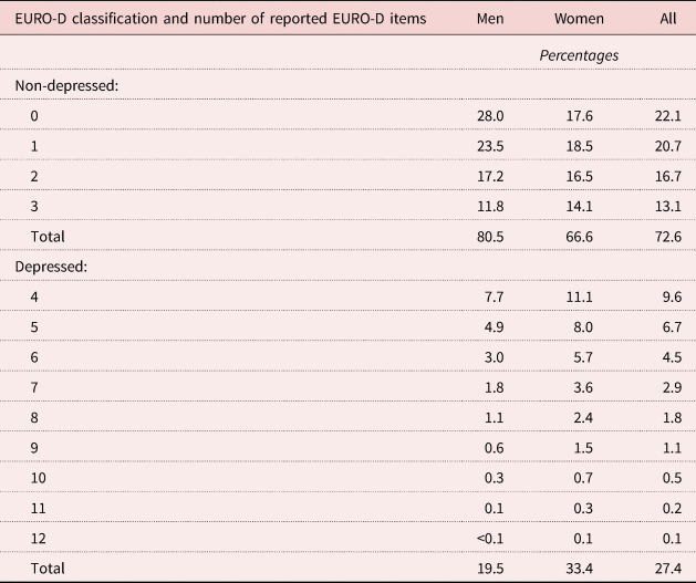
Results in Table 1 show that 27 per cent of respondents (20% of men and 33% of women) report being depressed according to the EURO-D scale. When we closely look at the combinations of the reported symptoms, we find that the majority of the depressed people indicate four or five items, and only a small proportion of them (for women it is larger than 7.5 per cent) report nine or more symptoms. The distribution of the reported disorders among respondents not classified as depressed shows a mode of zero for men and one for women: three items are indicated by more than 20 per cent of the old women and less than 15 per cent of men.
Table 1. Classification and total number of reported depressive symptoms according to the EURO-D scale, by gender
Figures 1 and 2 provide some information on the symptoms; the most reported are depression, sleep, irritability, fatigue and (only for women) tearfulness, the least reported are suicidality and guilt.

Figure 1. Distribution of the reported depression symptoms, by gender.

Figure 2. Distribution of the reported depression symptoms, by gender and EURO-D classification.
The same pattern on the most and least reported symptoms is found among depressed respondents and those reporting not being depressed according to the EURO-D scale.
The two-stage model solution
Several LC models over the 12 EURO-D items are estimated, varying the number of LCs. In Table 2 we show indices of model fit and performances. The information criteria (Akaike information criterion, Bayesian information criterion, etc.) are the most used indicators, however, in this case their values show very strong similarities across all estimated models (for instance, comparing the model with seven LCs with the one having ten more LCs, the differences are even lower than 0.1 per cent, for all indicators). Similar conclusions may be reached according to the classification errors statistics.
Table 2. Model fit indices of the Latent Class (LC) analysis over the depressive symptoms

Notes: AIC: Akaike information criterion. BIC: Bayesian information criterion. CAIC: Consistent Akaike information criterion. AIC3: Akaike information criterion with 3 as penalising factor. BVR: Bivariate Residual.
BVR values allow the violation of the local independence assumption to be checked. Models with 14 or fewer LCs present at least one large BVR (i.e. larger than 3.84). We add other classes to the models, first to guarantee that this assumption is met and then because a large number of classes may better capture particular and specific combinations of the reported symptoms.
Therefore, according to all criteria and indicators, the model with 15 LCs appears to be the best solution. Moreover, with respect to a model with a larger number of LCs, it is more parsimonious and shows only one class with a very small size (lower than 1%).
Table 3 shows the main results, that is the size of each cluster and the individual probabilities of reporting the depressive symptoms conditional to belong to the LC. Additional findings are available Tables B1 and B2 in the online supplementary material, in particular some demographic and socio-economic characteristics of the individuals belonging to each LC (since covariates are not specified as active in the model, the reported outcomes are based on the ex-post assignment of each respondent to the LCs).
Table 3. Latent Class (LC) analysis results: individual clusters and conditional probabilities of reporting depressive symptoms

The largest class (LC1) groups 37 per cent of the respondents and is characterised by a very low probability for all depressive and emotional symptoms. Figure 3 highlights that all individuals who do not mention any symptoms belong to this class, as well as people with at most two reported items. LC2, LC3 and LC8 are similar to each other, because they are characterised by people with a low probability in several items. The majority of respondents in these clusters report from one to three symptoms, but no more than five (LC3).

Figure 3. Distribution of the reported depression symptoms, by Latent Class.
Notes: The horizontal line shows the EURO-D cut-off. For each Latent Class a box plot is reported: the top of the rectangle indicates the third quartile and the bottom the first quartile, while a horizontal line within the rectangle indicates the median. A vertical line extends from the top of the rectangle to indicate the upper adjacent value (the most extreme value within 1.5 interquartile range of the nearer quartile) and another one from the bottom of the rectangle to indicate the lower adjacent value. Dots represent outliers.
These four classes are characterised by the lowest proportions of health problems (in particular for activities of daily living and mobility limitations) and a similar distribution by occupation (only in LC8 is the proportion of workers lower than in the other classes); the first three classes are similar also according to education. However, they differ according to age and gender: LC2 shows a large proportion of women, LC3 a slight majority of women, while LC1 and LC8 are the only two clusters in the analysis composed by a majority of males; LC1 and LC2 have the lowest average age among all LCs, while this value increases in LC3 and, particularly, in LC8. In LC1 individuals are more or less equally distributed by country, while an important role is played by Germany in LC2, Estonia in LC3 and Greece in LC8.
Also LC7, LC10 and LC14 are comparable, in the sense they are small (a total size of about 5.5% of people) and are characterised by individuals with a low probability for many depressive indicators and a quite large probability (i.e. higher than 0.5) for a couple of symptoms (for instance, depression and tearfulness in LC7 or fatigue and concentration in LC10). Moreover, each of these three classes groups large fractions of individuals from Belgium and Greece. LC10 and LC14 are also similar according to age (about 70 years on average), health status and occupation (large proportions of retired) of their individuals, while they differ by the proportion of women (larger in LC14) and low-educated people (larger in LC10). Respondents in LC7 are prevalently women, in fair health and show a proportion of low education and ‘other’ job status smaller than 50 and 8 per cent, respectively.
LC4, LC5 and LC6 include about 17 per cent of respondents having some probability of reporting a particular pattern of symptoms: depression, sleep, irritability and fatigue. The total number of cited items ranges from 3 to 9. LC4 and LC5 are also similar according to the poor health conditions (in particular for reporting at least two chronic diseases), education (more than 20% of individuals are highly educated) and occupation (the proportions of workers are larger than 20%), while the gender composition is very different: in LC5, as well as in LC6, we note the largest proportion of women (76.7%). In LC6 we observe a high average age (close to 70 years), even if the proportion of retired people is among the lowest across all LCs (there are indeed large percentages of homemakers and people in other occupational conditions).
To some extent, LC13 is similar to this group of classes (i.e. the range of the number of reported items), but the pattern of the symptoms having the highest probabilities is not exactly the same with respect to the previous one (for instance, in LC13 a key role is provided by pessimism). LC13 is mainly composed of very old (the average age is the highest among all classes) and retired people; there is just a slight majority of women. In this class we may also note large percentages of respondents living in Mediterranean countries and Estonia.
The remaining clusters (LC9, LC11, LC12 and LC15) are characterised by a large probability of several depressive indicators: the differences between each other involve the type and composition of such symptoms within each class (for instance, in the smallest class – LC15 – nine items show a probability higher than 0.7). About 99.5 per cent of respondents belonging to these LCs report a total number of items larger than three. LC11 and LC15 show some similar patterns according to age (the average value is larger than 73 years), occupation (low proportions of workers and large proportions of homemakers), education (more than 70% of their individuals are low educated) and countries of residence of their members (more than 50% of them live in the Mediterranean countries like Italy, Spain and Greece). Both classes report large proportions of health problems, higher in LC15 than in LC11. LC15 also identifies the group with the highest prevalence of women (about three-quarters of the sample). LC9 and LC12 are composed of individuals in poor health and a similar distribution according to education; however, in the former group respondents are, on average, much older (the difference is about 5.5 years) and largely retired than in the latter cluster. In LC12 more than one-third of individuals are from France, Belgium and Estonia; in LC9 about one-third of individuals are from Belgium, Italy and Estonia.
The individual probabilities of belonging to each class, computed in the LC analysis, are then used to perform FA, in order to identify a reduced number of clusters. Results of the FA are summarised in Tables 4 (eigenvalues and the proportion of explained variance by each factor), while Table 5 shows the factor loadings matrix of the chosen solution, after a Varimax rotation. According to the size of the eigenvalues (larger than 1), five factors should be retained; however, such solution allows explanation of only 56.5 per cent of the total variance. Based on the aims of our analysis, we believe that a greater proportion of variance needs to be explained – at least two-thirds of it. For this reason, we opt for the solution of seven factors, which also appears as a not so large number of depression categories.
Table 4. Eigenvalues and proportion of explained variance of the Factor Analysis for the solution with 15 Latent Classes

Table 5. Factor loadings of the Factor Analysis for the solution with 15 Latent Classes (after Varimax rotation, only loadings larger than 0.5 are reported)

Table 6 summarises the size of each retained factor, as well as their composition in terms of the original LCs (from one to four of them). According to the features of these LC compositions, we classify the respondents in the following categories: very low risk of depression, low risk of depression, middle risk of depression, high risk of depression, depressed, severely depressed and extremely depressed.
Table 6. Categories obtained according to our approach based on 15 Latent Classes (LCs)

Some demographic and socio-economic characteristics of the individuals belonging to each category are reported in Table C1 in the online supplementary material.
The very low risk and the middle risk of depression categories are similar according to age (the lowest average values), education (a more or less equal distribution) and occupation, in particular with the highest proportion of workers (nearly 30%). However, the former category is composed by healthier individuals than the latter; then, in the very low risk of depression group we note a slight majority of men (about 52%), whereas females are largely present in the other category. In the low risk of depression cluster we may underline the highest percentage of men among all categories, as well as very large proportions of low educated (more than half) and retired people (about 64%): the average age is high (close to 70), but not so large as in other groups. Interestingly, the low risk and the middle risk of depression categories show very similar distribution according to the health dimension. The high risk of depression category is mainly composed of unhealthy respondents (for instance almost 60% of them report two or more chronic diseases, while about one-third has at least three mobility limitations) and women (more than 60%). However, with respect to other traits, such as age, occupation and education, we may observe some similarities with the very low risk of depression category.
The depressed, severely depressed and extremely depressed groups are composed of very unhealthy individuals (according to all reported health conditions). Moreover, the very small-sized extremely depressed category stands out compared to the others, because it shows the highest proportion of women, low educated and homemakers and, at the same time, the lowest proportion of workers and average household sizes. The depression category is composed of very old (the average age is larger than 73), mainly retired and low-educated respondents, even if the proportion of women is not so large as in other clusters. Individuals belonging to the severely depressed category are younger, more educated and with a higher proportion of workers than the depressed and extremely depressed groups; we may also note a very strong majority of women (more than 70%).
Robustness checks
In this section we aim to compare the main similarities and differences in the individual classification according to our approach and the EURO-D indicator. Findings are indeed very interesting and strengthen our results.
According to Figure 4, all respondents in the extremely depressed category and nearly all in the depressed and severely depressed categories are classified as depressed also by the EURO-D scale. Gender differences do not appear, in contrast with the evidence within each of the other categories, where the proportion of women classified as depressed according to the EURO-D scale is larger than the one of men. From the high risk of depression to the very low risk of depression categories, the prevalence rate of depressed people according to the EURO-D instrument is lower and lower, reaching a minimum in the very low risk of depression cluster equal to 3.7 and 6.5 per cent for males and females, respectively. The middle risk and the high risk of depression clusters show the largest differences by gender.

Figure 4. Proportion of the older people classified as depressed according to the EURO-D scale within each category identified according to our approach, by gender.
These conclusions are appealing, but do not take into account differences in sizes among the categories obtained through our approach. To this aim, Figure A1 in the online supplementary material shows the distribution of our seven categories within each group of older people classified as depressed and non-depressed by the EURO-D scale (by gender).
About 55 per cent of individuals defined as non-depressed according to the EURO-D scale fall into either the very low risk or the low risk of depression category. There is, however, a distinction between male and female respondents: 58 per cent of men and 48 per cent of women are in the very low risk of depression category. A similar result (but opposite in sign) arises for the middle risk of depression cluster. For the remaining categories of the non-depressed people there are no differences by gender and, in particular, less than 0.25 per cent of respondents are classified in any category from depressed to extremely depressed in both samples. In such cases, it is interesting to underline that all individuals (regardless of the gender) identified as non-depressed by EURO-D and severely depressed by our approach report the same pattern of symptoms: depression, pessimism and wishing death.
Conditionally to the depressed group of people obtained according to the EURO-D instrument, no relevant gender differences appear: about 15 per cent of men and 17 per cent of women are in the categories from very low risk of depression to middle risk of depression; about 28 per cent of men and 25 per cent of women lie in the categories from depressed to extremely depressed. More than half of the individuals identifying as depressed by the EURO-D scale are classified as at high risk of depression according to our approach.
To summarise, all of these results highlight that a large proportion of individuals classified as depressed according to the EURO-D instrument falls in any of our clusters that we have labelled at some risk of depression, with men and women who behave similarly. Furthermore, a non-trivial proportion of older people classified as non-depressed by the EURO-D scale are identified as at some risk of depression according to our approach, but, in this case, some gender differences arise.
If we assume as a benchmark the depression status provided by the EURO-D instrument, we might evaluate the goodness of our findings constructing the ROC curve of our classification (Figure A2 in the online supplementary material): the area under the ROC curve is about 0.85, which is a quite good result.
Additionally, in a sensitivity analysis we explore how the results change when choosing a different LC solution, that is, according to the set of indicators, the model with 16 classes. Applying FA to the probability of belonging to each class, the solution with seven factors explains about 66 per cent of the total variance: in this FA, six eigenvalues are larger than one, while the seventh is equal to 0.984. Exploiting the matrix containing the factor loadings, the retained factors are then constructed as for the model with 15 LCs and the first encouraging result is that we may apply the same labels of the previous classification also to this solution.
Table D1 in the online supplementary material compares the concordance in class belonging of all individuals: more than 95 per cent of people identified as at low risk and at middle risk of depression in the classification based on 15 LCs are in the same categories also according to the classification based on the 16 LCs model. Very large values may be obtained also for the two extreme categories of the classification. Overall, 79.5 per cent of all individuals are identified in the same category in both solutions and this result is better for males (82.0%) than females (77.7%), as we can see from Tables D2 and D3 in the online supplementary material. Some problems arise for people classified as severely depressed by the 15 LCs solution: less than 10 per cent of them are in the same category also for the 16 LCs model, while the largest proportion of them belong to the high risk of depression cluster according to the 16 LCs solution. Similarly, we may note concordance of classification in the high risk of depression category for about 60 per cent of people identified by the 15 LCs estimates, while about 30 per cent are classified in any category from very low risk to middle risk of depression according to the 16 LCs findings. However, as before, in order to comment correctly on this comparison, we have to take into account also the large size differences across these categories.
Looking at Tables D2 and D3 in the online supplementary material, 3.2 per cent of male respondents (4.4% of females) classified in any category from depressed to extremely depressed according to the model with 15 LCs are assigned to any category from very low risk of depression to high risk of depression by the model with 16 LCs. On the other hand, only 2.1 per cent of males (4.9% of females) assigned to the high risk of depression or a lower category by the 15 LCs solution are identified as depressed (or at higher level) by the other estimation.
Discussion
Using a combination of LC modelling and FA we are able to identify seven categories of depressive and emotional problems, from a very low risk of depression cluster to a group of extremely depressed people. These clusters are characterised by different and interesting mixes of symptoms and these differentiations may help epidemiologists, clinicians and health researchers to better observe and understand the presence and the severity of any manifestations of depression among older adults. Moreover, a pithier classification (instead of the classification into a large number of clusters, some of them of small size, as provided by the LC analysis at the beginning) could be more effective, in practice, for use by any health operators.
However, it is important to note that our categories are not defined (both in number and/or in main features) a priori. Individuals are grouped according to the likelihood of observing certain patterns of reported items and people are assigned to the classes on the basis of probabilistic criteria. This means that in each category we may find individuals characterised by different patterns of symptoms, but the model-based solution guarantees that such patterns have nonetheless some common traits. To this aim, in the present analysis we have labelled the categories according to some features (that is, the combination and the number of some reported disorders) of the LCs belonging to each factor. However, clinicians or other experts may rename these categories in a different way, according to the presence (or not) of other specific characteristics, symptoms or general patterns in which they have interest (for instance, the occurrence of sleeping and fatigue problems or the presence of medical comorbidities in the created groups, and so on).
As a consequence, the final output of our approach has to be analysed in empirical researches as a categorical (non-ordinal) variable. However, from a practical point of view, there are no substantial differences with respect to the use of a binary indicator constructed according to a cut-off measure: if it acts as an explanatory variable, many dummy regressors from our categorical variable may be created and introduced in the analysis. If specified as a dependent variable, a multinomial distribution might be assumed for modelling (this is true also if the model suffers from endogeneity problems, such as reverse causality issues that often apply, for instance, when analysing the relationship between health and socio-economic status among older people).
According to our taxonomy, about 40 per cent of the total population is classified at a very low risk of depression. All individuals in this cluster present a similar pattern or combination of such symptoms (i.e. no or just one or two reported items). On the other hand, the last three categories are characterised by individuals with a high probability of reporting several depressive and emotional problems. It is likely that in such cases depression corresponds to a clinical diagnosis. The other three categories range from low risk of depression to high risk of depression: more than half of respondents are in these categories. One-third of respondents fall into the high risk of depression category: these individuals are not yet classified as depressed, but should be monitored to prevent future development of depression.
Gender differences are quite apparent. We observe that nearly half of the older men are in the very low risk of depression category, while less than 6 per cent are classified in the last three categories of depression. Instead, a considerably lower proportion of women than men are in the very low risk of depression group. The greatest gender difference is found in the middle risk of depression cluster: the number of female respondents who fall into this category is about 1.5 times larger than the one for men. However, the gender difference reduces to only 2 per cent in the categories from depressed to extremely depressed.
Furthermore, we show interesting comparisons between the approach we adopt and the cut-off point approach of the EURO-D scale. We show that people classified as depressed by the EURO-D scale present different depression characteristics, e.g. a large proportion of these individuals (primarily women) are in the high risk of depression or a lower category according to our approach. Therefore, our findings can be helpful to investigate further heterogeneity in the manifestation of late-life depression.
Lastly, in order to strengthen the potentialities of our approach, Table E1 in the online supplementary material reports the results of regression model estimations that compare the use of the single indicator of depression based on the cut-off value of the EURO-D scale and the categories created by our solution. We use SHARE Wave 6 data to investigate the relationship between cognitive abilities and depression (no causal effects), as in Portellano-Ortiz and Conde-Sala (Reference Portellano-Ortiz and Conde-Sala2018). The dependent variable in each estimated model is the result of the fluency test, which provides a measure of individual cognitive abilities (this variable counts the total number of animals cited by the respondent in one minute); several individual and household characteristics (gender, age, education, household size, physical health, job status, country) are specified for controlling. Other things being equal, a negative relationship between depression and cognitive abilities appears. However, the specification of a single dummy variable for depression (based on the EURO-D cut-off) cannot introduce in the model some forms of non-linearities in the analysed relationship that our approach may instead provide (an alternative solution that supports this finding is also estimated, that is a model where depression is investigated by means of a continuous variable created as the total number of reported items of the EURO-D scale). Another interesting result that strengthens the potentialities of our approach is that the old individuals with the largest (negative) estimates belong to four categories (low risk of depression, depressed, severely depressed and extremely depressed), having a common trait according to the LC profiling, that is a not trivial probability of reporting the pessimism symptom.
Strengths and weaknesses
The main strength of the approach used is the identification of several levels of severity of the depressive disorders, that goes beyond the simple dichotomisation of depression (present or not).
Furthermore, this approach allows flexibility in labelling each category that was obtained, according to the nature, type and number of the mental disorders under investigation. Another major strength is that this approach can be easily applied to data collected by any depression instrument, other than the EURO-D scale, designed to detect the presence or the absence of certain symptoms or emotional disorders. Lastly, given that the approach is strongly model-driven, subjective evaluation is limited.
Several limitations should be also acknowledged. In factor analysis we could only explain a proportion of the whole variance, nevertheless, it is remarkable the high values of agreement rates between the two solutions we have compared, and the few large discrepancies in the category assignments. Second, in the LC estimation, no active covariates have been specified, but they may be easily introduced to generate the LCs. Third, we have limited our approach to cross-sectional data for the sake of clarity. However, given the dynamic nature of depression (which often has a chronic course), researchers could be even more interested in modelling developmental trajectories (i.e. the course of a behaviour over age or time) or patterns of change in these outcomes across multiple time-points. LC models can be easily extended to longitudinal data (dynamic segmentation). In this context, promising approaches involve the development and the estimation of Latent Class Growth Models or Latent Class Markov Models, in order to allow units to change over time the group to which they belong. Lastly, FA seems the most suitable technique for clustering the probabilities obtained after the LC analysis, because its application is straightforward and allows highlighting of combinations of patterns of depressive symptoms with some common traits. Other solutions are, however, suitable, such as building a composite indicator, in particular if some of the 12 EURO-D items might be considered more important than some others.
Conclusions
We have shown that is possible to use a model-based approach for classifying individuals in a more accurate way than the simple dichotomisation ‘depressed’ versus ‘non-depressed’. Homogeneous groups of people with different levels of depressive or emotional symptoms could be highlighted, in particular those who are at (lower or higher) risk of developing depression. On the one hand, this refined classification of older individuals may provide the basis for improving current protocols for detecting different levels of depressive disorders and helping to develop customised intervention and treatment programmes. On the other hand, this approach may be applied as a new way to investigate further the heterogeneity of depressive symptoms among the older population, both in replications of already-published studies and in new empirical analyses; for instance, taking into account comorbidity issues, researchers may have interest in probing whether such categories, identified at early old age, may be stable over time or may be good predictors of the onset of some forms of physical or working disabilities in later life.
Supplementary material
The supplementary material for this article can be found at https://doi.org/10.1017/S0144686X19001077
Acknowledgements
The authors thank Luca Grassetti for his helpful comments and suggestions. Earlier versions of this paper were presented at the Biostatistics Network Seminar, UCL Research Department of Statistical Sciences (London, 2015) and the Satellite Workshop – 4th Health Econometrics Workshop (Padua, 2014). The authors are grateful to all participants at these conferences and seminars.
Financial support
This study was partially supported by the project ‘Care, Retirement & Wellbeing of Older People Across Different Welfare Regimes’ (CREW). The SHARE data collection has been funded by the European Commission through FP5 (QLK6-CT-2001-00360), FP6 (SHARE-I3: RII-CT-2006-062193, COMPARE: CIT5-CT-2005-028857, SHARELIFE: CIT4-CT-2006-028812), FP7 (SHARE-PREP: GA N°211909, SHARE-LEAP: GA N°227822, SHARE M4: GA N°261982) and Horizon 2020 (SHARE-DEV3: GA N°676536, SERISS: GA N°654221) and by DG Employment, Social Affairs & Inclusion. Additional funding from the German Ministry of Education and Research, the Max Planck Society for the Advancement of Science, the U.S. National Institute on Aging (U01_AG09740-13S2, P01_AG005842, P01_AG08291, P30_AG12815, R21_AG025169, Y1-AG-4553-01, IAG_BSR06-11, OGHA_04-064, HHSN271201300071C) and from various national funding sources is gratefully acknowledged (see www.share-project.org).


