2.1 Model overview

The coaxial compound helicopter model utilized in this article is based on the model described by Yuan^{(Reference Yuan, Thomson and Chen21)}, which has been verified with flight test data and simulation result from other researcher. The model is composed of five parts: rotor, propeller, horizontal tail, vertical tail, and fuselage.

In the rotor part, a conventional disc-type model is used to calculate the rotor forces and moments. The induced velocity model is based on the Pitt-Peters dynamic inflow model and assumes the induced inflow of the lower rotor does not affect the upper rotor’s ability to generate thrust, and the rotors are sufficiently close together that the wake from the upper rotor does not fully develop^{(Reference Ferguson and Thomson20,Reference Ferguson and Thomson22–Reference Gaonkar and Peters24)} . In addition, due to the rigidity of the coaxial rotor system, it is reasonable to assume in developing the rotor model, we ignore the pitching and lagging degree of freedoms (DOFs), and that the flap motion has the most influence on the flight dynamics characteristics. To simulate the flapping motion more precisely, the model utilizes the equivalent flapping offset and flapping spring method, and the detail of the simplify method is shown in reference⁽²¹⁾. According to this method, the rigidity of the equivalent flapping spring ${K_{10}}$ can be written as:

(1) \begin{equation} K_{10} =\left(\overline{\omega }_{n}^{2} -1-\frac{\overline{e}RM_{\beta } }{I_{\beta } } \right)I_{\beta } \Omega ^{2} \label{eqn1} \end{equation}

where: ${\overline{\omega }_{n} }$ is the non-dimensional rotor flapping frequency, which is equal to ${\omega _{n} /\Omega R}$ . It should be mentioned that ${\Omega}$ is the rotor rotational speed, and it may change with forward speed based on the variable rotor speed strategy; ${\overline{e}}$ is the equivalent flapping offset; R is the rotor radius; ${M_{\beta } ,I_{\beta } }$ are the blade mass static moment and blade moment of inertia, respectively. Based on the relationship between the rotor speed and the first-order flapping frequency of the coaxial rigid rotor^(25,26) (shown in Fig. 1), ${\overline{\omega }_{n}}$ should be a variable with respect to ${\Omega }$ . Thus, using a fitting method, ${\overline{\omega }_{n}}$ can be obtained by:

(2) \begin{equation} \overline{\omega }_{n} =\overline{\omega }_{n,0} \left(1+\eta \frac{\Omega _{ori} -\Omega }{\Omega _{ori} } \right) \label{eqn2} \end{equation}

where: ${\overline{\omega }_{n,0} }$ is the original non-dimensional flapping frequency of the coaxial rigid rotor, and ${\eta }$ is the influence factor, which reflects the relationship between the non-dimensional flapping frequency and the rotor rotational speed, and its value can be obtained on the basis of Fig. 1. During the modelling process of the flapping feature, Eq. (2) is firstly calculated to determine the flapping frequency of the coaxial rigid rotor. Then, this frequency is put in Eq. (1), and consequently the effect of the rotor rotational speed is considered in the rotor flapping model.

Figure 1. Relationship between non-dimensional first-order flapping frequency and rotor speed^{(Reference Feil, Rauleder and Hajek26)}.

Meanwhile, an airfoil aerodynamic look-up table is utilized in aerodynamic load calculation of the rotors. The aerodynamic modelling of the propeller is similar to that of the rotor except that no flapping motion is involved in the propeller section. In addition, 2-D representations of the horizontal and vertical tails with strip theory are incorporated into the model. The lift and drag coefficients can be obtained from 2-D airfoil aerodynamics look-up tables with given angles of attack and sideslip. The fuselage model uses data from wind tunnel tests⁽²⁷⁾. The force and moment coefficients of the wind tunnel experiment are dependent on the fuselage angles of attack and sideslip.

The flight dynamics model of the coaxial compound helicopter contains 24 DOFs. The state-space equations of the model can be expressed as:

(3) $$\dot{\mathbf{\mathit{x}}}=f(\mathbf{\mathit{x}},{\mathbf{\mathit{u}}},t)$$

where ${\mathbf{\mathit{x}}=[\mathbf{\mathit{E}},\mathbf{\mathit{F}},\mathbf{\mathit{G}},\mathbf{\mathit{H}}]^{T}}$ , ${\mathbf{\mathit{E}}=[u,v,w,p,q,r,\phi ,\theta ,\psi ]^{T}}$ represents the velocity, the angular velocity, and the Euler angle of the fuselage; ${\mathbf{\mathit{F}}=[\beta _{L0} ,\beta _{Lc} ,\beta _{Ls} ,\beta _{U0} ,\beta _{Uc} ,\beta _{Us} ]^{T} }$ is the lower and upper rotors’ flapping angles; ${\mathbf{\mathit{G}}=[v_{L0} ,v_{Lc} ,v_{Ls} ,v_{U0} ,v_{Uc} ,v_{Us} ]^{T}}$ is the lower and upper rotors’ induced velocities; ${\mathbf{\mathit{H}}=[v_{p0} ,v_{pc} ,v_{ps} ]^{T} }$ is the induced inflows of the propeller. ${\mathbf{\mathit{u}}{\rm =[}\theta _{{\rm 0}} ,\theta _{1c} ,\theta _{1s} ,\theta _{01} ,\theta _{dc} ,\theta _{p} ,\Omega ]^{T} }$ is the control inputs of the coaxial compound helicopter; ${\theta _{{\rm 0}} }$ is the collective; ${\theta _{1c} }$ is the lateral cyclic pitch; ${\theta _{1s} }$ is the longitudinal cyclic pitch; ${\theta _{01} }$ is the collective differential; ${\theta _{dc} }$ is the differential lateral cyclic pitch; ${\theta _{p} }$ is the collective of the propeller.

In order to calculate the handling qualities, Eq. (3) can be linearized as:^{(Reference Ferguson and Thomson20)}

(4) \begin{equation} \dot{\mathbf{\mathit{x}}}_{linear} =\mathbf{\mathit{Ax}}_{linear}+ \mathbf{\mathit{Bu}}_{linear} \label{eqn4} \end{equation}

where: ${\mathbf{\mathit{x}}_{linear} =[u,v,w,p,q,r,\phi ,\theta ]^{T}}$ is the state vector in linearization; $\mathbf{\mathit{u}}_{linear}={[ \theta _{{\rm 0}} ,\theta _{1c}, \theta _{1s} ,\theta _{01} ]^{T} }$ is the control vector in linearization in this article. The system matrix, A, contains the stability derivatives whereas the control derivatives define the control matrix, B. The elements in these two matrixes can be obtained using numerical differentiation method with Eq. (5) and Eq. (6), which are:

(5) \begin{equation} \mathbf{\mathit{A}}=\left[\frac{\partial f}{\partial \mathbf{\mathit{x}}_{{\it linear}} } \right]_{x=x_{0} } \label{eqn5} \end{equation}

(6) \begin{equation} \mathbf{\mathit{B}}=\left[\frac{\partial f}{\partial \mathbf{\mathit{u}}_{{\it linear}} } \right]_{x=x_{0} } \label{eqn6} \end{equation}

where: ${x_{0} }$ represents the state vector at given flight range, and the detail of this reduction process is shown by Padfield^{(Reference Padfield7)}.

The aircraft data used in this article is based on the XH-59A helicopter. The primary data for the XH-59A helicopter is shown in Table 1^{(Reference Ferguson23,Reference Ruddell28)} . The related parameters are in the body coordinate, which origin point is at the center of gravity. The X direction of this coordinate points at the nose of the vehicle, and the Y direction points at the right. The Z direction is set based on the right-hand rule.

The XH-59A helicopter utilized an auxiliary propulsion unit rather than a propeller to provide the thrust in high-speed flight. This article uses a propeller instead, which is more in line with the development of coaxial compound helicopters in recent years. The parameters of the propeller are shown in Table 2^{(Reference Ferguson23)}.

Table 1 XH-59A helicopter parameters

Table 2 Parameters of compound propeller

2.2 Engine model

In this article, the maneuver characteristics with a variable rotor speed strategy will be investigated. Therefore, a rotorspeed governer/engine model should be included in the flight dynamics model during the maneuver investigation. The simplified model and parameters used in this article are described by Padfield^{(Reference Padfield7)}, where the transfer function between rotor torque and rotor speed can be expressed as follow:

(7) \begin{equation} \frac{\overline{Q}_{e} (s)}{\overline{\Omega }(s)} =G_{e} (s)H_{e} (s) \label{eqn7} \end{equation}

where: ${\overline{Q}_{e} }$ is the non-dimensional turbine engine torque output at the rotor gearbox. ${G_{e} (s)}$ is related to the change in rotor speed with the fuel flow, which can be represented as a first-order lag:

(8) \begin{equation} G_{e} (s)=\frac{K_{e1} }{1+\tau _{e1} s} \label{eqn8} \end{equation}

where: the time constant ${\tau _{e1} }$ determines the speed of the fuel being pumped into the turbine, it can be set as 0.1s^{(Reference Padfield7)}. The gain ${K_{e1} }$ can be selected to give a prescribed rotor speed droop from flight idle fuel flow to maximum contingency fuel flow. ${H_{e} (s)}$ is the transfer function between the fuel and the required engine torque, which is shown as follow:

(9) \begin{equation} H_{e} (s)=K_{e2} \left(\frac{1+\tau _{e2} s}{1+\tau _{e3} s} \right) \label{eqn9} \end{equation}

where: gain ${K_{e2} }$ can be set to give 100% ${\overline{Q}_{e} }$ at some value of fuel flow, thus allowing a margin for maximum contingency torque. ${\tau _{e2} ,\tau _{e3} }$ are the engine lead and lag time. ${\tau _{e2} }$ is assumed to be invariable with torque, and its value is set as 0.08 s^{(Reference Padfield7)}. ${\tau _{e3} }$ can be expressed as a function of the rotor torque^{(Reference Padfield7)}:

(10) \begin{equation} \tau _{e3} \approx \tau _{e30} +\tau _{e31} \overline{Q}_{e} \label{eqn10} \end{equation}

In this equation, the value of ${\tau _{e30} }$ is 0.6 s and ${\tau _{e31} }$ is ${-}0.4$ s^{(Reference Padfield7)}.

Therefore, Eq. (10) can be written as Eq. (11) in time domain:

(11) \begin{equation} \ddot{Q}_{e} =-\frac{1}{\tau _{e1} \tau _{e3} } \{ (\tau _{e1} +\tau _{e3} )\dot{Q}_{e} +Q_{e} +K_{3} (\Omega -\Omega _{i} +\tau _{e2} \dot{\Omega })\} \label{eqn11} \end{equation}

where: ${K_{3} =K_{e1} K_{e2} }$ . Therefore:

(12) \begin{equation} \dot{\Omega }=\dot{r}+\frac{1}{I_{R} } (Q_{e} -Q_{r} -g_{p} Q_{p} ) \label{eqn12} \end{equation}

where: ${\dot{r}}$ is the angular acceleration around the yaw axis; ${I_{R} }$ is the combined moment of inertia of the rotor hub and blades and rotating transmission to the free turbine; ${g_{p}}$ is the propeller gearing, and ${Q_{p} }$ is the propeller torque.

2.3 Trim strategies

In this article, the performance, handling qualities, and maneuver characteristics will be analyzed. The starting point of these analysis is the trim state. The trimming process for a coaxial compound helicopter is slightly different from conventional helicopter as the trim strategy of the propeller and LOS have to be included.

The auxiliary propeller is used to provide thrust at high-speed flight range to improve the performance of the coaxial compound helicopter. The propeller thrust is, therefore, an additional unknown variable in the trim process. This coaxial compound helicopter utilizes the propeller collective ${\theta _{p} }$ to control the thrust provided by the auxiliary propeller. Thus, a fuselage pitch attitude schedule⁽²³⁾ is used in the trim strategy, and the propeller collective can be used as a trim target during the trim process.

Since LOS is adopted in the coaxial compound helicopter, the lift-center moves towards the advancing side and consequently, the dynamic stall problem can be prevented. The LOS value can be defined as Eq. (13) ^{(Reference Burgess8)}.

(13) \begin{equation} \mathit{LOS}=\frac{M_{x,L} -M_{x,U} }{TR} \label{eqn13} \end{equation}

where ${M_{x,L} ,M_{x,U} }$ are the rolling moment of lower and upper rotors respectively, and T is the thrust of the coaxial rotor system.

LOS can be regulated by differential lateral cyclic pitch, ${\theta _{dc} }$ . Therefore, this control input is used to guarantee LOS value to follow Eq. (14) in different forward speeds^{(Reference Ferguson23)}.

(14) \begin{equation} \mathit{LOS}=0.00002v_{f} ^{2} \label{eqn14} \end{equation}

Eq. (14) derives from the wind tunnel and flight test of X2TD helicopter^{(Reference Walsh, Weiner, Arifian, Lawrence, Wilson, Millott and Blackwell29)}, in which the different LOS value have been evaluated as forward speed increases. The results indicate that the LOS should increase with the forward speed. Therefore, reference 23 concludes this trend using Eq. (14), which could guarantee the rotor efficiency at various flight ranges. When the helicopter is in hover and low-speed forward flight, the dynamic pressure of the advancing and retreating sides are similar. The LOS value should remain relatively low to improve the efficiency of the rotor. As forward speed increases, the dynamic pressure of the advancing side is higher, and LOS should also increase to avoid the dynamic stalling at the retreating side.

The main research objective of this article is to investigate the effect of an improved variable rotor speed strategy. Thus, the original variable rotor speed strategy (Fig. 2) can be used for comparison^{(Reference Bagai19,Reference Ferguson and Thomson22)} .

Figure 2. Original variable rotor speed strategy.

As indicated in Fig. 2, the original rotor speed strategy is designed to avoid compressibility effects at the advancing blade tip in high-speed flight.

2.4 Inverse simulation method

Inverse simulation is an efficient method to investigate the maneuver characteristics of a helicopter. This method is explained widely in the literatures by various authors^{(Reference Hess, Wang and Gao30–Reference Thomson and Bradley33)}. Therefore, only a brief overview of this method is shown in this article.

The forward time response solution of inverse simulation is readily available when the flight dynamics model is constructed. The inverse simulation can be represented as a “trim process” with respect to each time steps through a predefined trajectory or maneuver. At the new time increment, the control input must be varied to maintain the correct flight path, which is given by the requirement of the Mission-Task-Element (MTE)^{(Reference Standard34)}.

To process the inverse simulation algorithm, this article executes the following steps with respect to the characteristics of the coaxial compound helicopter with LOS rotors:

1) Calculate trim control inputs

The trim state is the initial point of the maneuvers. The trim variables of the conventional helicopter are equal to the trim target equations. However, the coaxial compound helicopter has redundant control inputs, which further complexes the trim process. Thus, the trim strategies mentioned above are utilized here to determine the initial point of MTE.

2) Define the maneuver

The maneuver can be defined simply by polynomial representations of position or other flight path variables and is then discretized into a series of discrete time points. The redundant controls of the helicopter may affect the definition of the maneuver as they may need additional boundary conditions to determine the control inputs in every time step. Therefore, the strategies of redundant control inputs utilizes the trim strategies mentioned above at each time step.

3) Calculate control vector

This inverse simulation model uses a Newton-Raphson technique to calculate the controls required to maintain the helicopter’s states in accordance with the maneuver mathematical description. This process is repeated throughout each time-step until the maneuver has been completed.

3.0 VARIABLE ROTOR SPEED STRATEGY

3.1 Performance investigation

The power required results with different rotor rotational speeds at various forward speeds are shown in Fig. 3, in which the rotor speed ratio means the ratio between the rotor speed adopted, $\Omega$ , and the original rotor speed, $\Omega_{st}$ , from Table. 1.

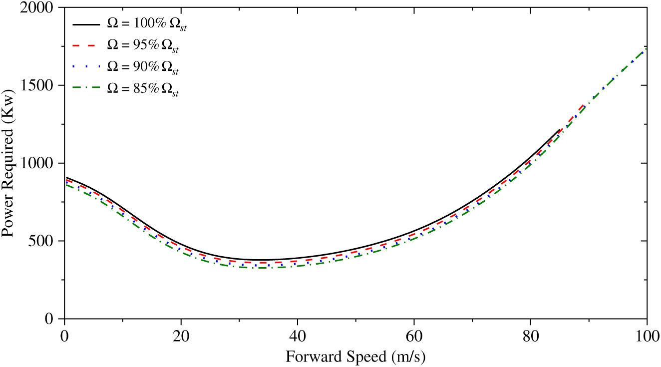
Figure 3. Overall power required (rotor and propeller) with different rotor speed.

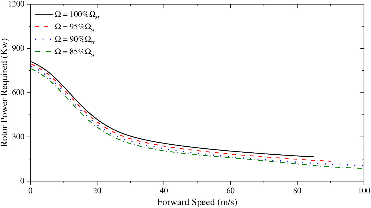
As indicated in Fig. 3, the helicopter cannot trim in high-speed flight with the rotor speed of 35.9 rad/s due to the compressibility effect on the advancing blade tip. It also accounts for the decrease in the original rotor speed strategy at high-speed flight range. In addition, the power consumption is reduced with variable rotor speed, which is more significant in the low- to mid-forward speed range, but not obvious in high-speed flight. In order to understand this phenomenon, the rotor power consumption of the coaxial rotor system is shown in Fig. 4.

Figure 4. Rotor power required with different rotor speed.

Figure 4 shows that the power consumption of the rotor is reduced in high-speed flight and the propeller mainly provides the thrust that the helicopter needs to trim. This figure demonstrates that although reducing rotor speed drops down the rotor power required, the overall power required does not change significantly as the propeller requires significant power in this flight range. In addition, the variable rotor speed couples with the propeller, and the thrust provided by the propeller may also change with the rotor speed. Thus, the variable rotor speed may also influence the power consumption of the propeller.

3.2 Rotor speed strategy in trim flight

The aim of the variable rotor speed for the coaxial compound helicopter is to reduce the power consumption across the flight range. Therefore, the rotor speed strategy is formulated to a single input and single output (SISO) problem at every speed point.

On the other hand, a correction needs to be made for the LOS trim strategy based on Eq. (14). The change of the rotor rotational speed could influence the dynamic pressure difference between the advancing and retreating sides. Therefore, it would be better to use the advancing ratio to calculate the LOS value at different flight speeds, which could take the effect of rotor rotational speed into account. As the rotor tip speed in the original state is around 200 m/s, the LOS control strategy can be obtained considering the rotor rotational speed, which is shown in Eq. (15).

(15) \begin{equation} LOS=0.00002v_{f}^{2} =0.8\left(\frac{v_{f} }{\Omega R}\right)^{2} =0.8\mu ^{2} \label{eqn15} \end{equation}

The aim of Eq. (15) is to improve the efficiency of the coaxial rotor system at various flight velocities considering the variable rotor speed. The LOS value is decided by the dynamic pressure difference between the advancing and retreating rotors. In fact, this difference is determined by both the forward speed and rotor rotational speed. In other words, when the rotor rotational speed decreases, the retreating side has more possibility to be in the dynamic stalling at given LOS value. Therefore, the advancing ratio should be utilized to define the LOS setting. Based on Eq. (15), the optimized rotor speed is shown in Fig. 5. Also, the trim limits of the variable rotor speed are also given in this figure.

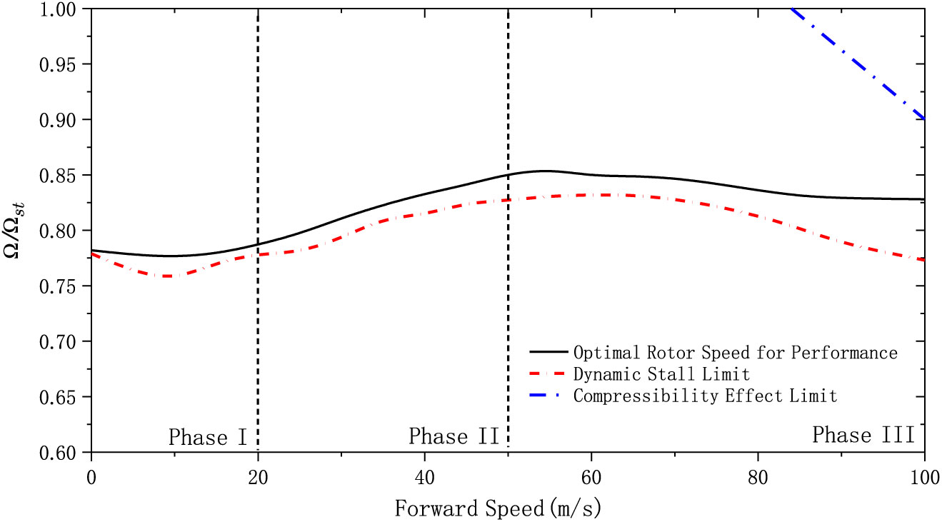
Figure 5. The optimal rotor speed for performance with various rotor speed.

The trend of the final rotor speed strategy is similar to that observed in other research^(13,15). These references are based on the conventional helicopter, but the similarity helps verify the results in this article. On the other hand, the rotor speed limit changes significantly across the flight range. The lower limit line is due to the dynamic stall. When the rotor speed is lower than this limit, the flapping effect is significant due to the increase of the collective pitch and advancing ratio. Therefore, most blade elements on the retreating side will be in the stalled condition, and insufficient thrust is provided to maintain the trimmed state. The upper limit in high speed is to prevent the advancing side of the rotor disc from the compressibility effect. When the rotor speed is relatively high, the Mach number of the advancing blade tip would be close to the limit of the compressibility, which increases the overall power consumption and lead the helicopter to be unable to achieve the trim status. Meanwhile, the trend of upper limit is similar to the original rotor speed strategy in Fig. 2, which further proves the accuracy of the results in Fig. 5.

Based on the rotor speed change, the rotor speed strategy can be divided into three phases for analysis.

3.2.3 Phase III (high-speed forward flight)

In this flight range, the rotor speed stops increasing and drops down slightly with forward speed. Firstly, the compressibility effect requires the rotor speed to reduce. In addition, the efficiency of the propeller becomes higher with forward speed increases, and the thrust of the rotor is reduced, which would further influence the optimized rotor speed. It also should be mentioned that the upper limit only takes effect at this flight range because the compressibility effect only occurs when the Mach number is above 0.75.

With the rotor speed strategy in Fig. 5, the power required comparison with the original strategy is shown in Fig. 6. According to the power required comparison results, this rotor speed strategy could reduce the power consumption, especially in mid-speed forward flight. In other words, the cruise-efficiency and flight duration can be improved by this rotor speed strategy. It demonstrates that the power required could be reduced by around 15% compared with the original strategy when the forward speed is around 35m/s. In the high-speed flight, the effect is not obvious. The reduction is only 1.2% when the speed is around 100m/s. Furthermore, the reduction of the power consumption is around 10% of the original power required in hover and low-speed forward flight. However, the rotor speed is close to the limit at this flight range and so there could be degradation in the maneuverability if the collective is not associated with the rotor speed. Meanwhile, according to Fig. 5, the optimized range of the rotor speed change is not significant. It may be argued that a fixed rotor speed would be sufficient for this helicopter. Thus, the power required of 85% ${\Omega _{st} }$ is also added in Fig. 6 as a comparison. The results indicate that the proposed variable rotor speed strategy could further reduce the overall power required compared to the 85% ${\Omega _{st} }$ case, especially in hover and low-speed forward flight. It should be mentioned that if the rotor speed is fixed at 85% ${\Omega _{st}}$ across the flight range, the maneuverability of this helicopter would be degraded to a large extent because the coaxial rotor is close to the stalling condition and cannot use the variable rotor speed strategy to provide sufficient thrust in maneuvering flight.

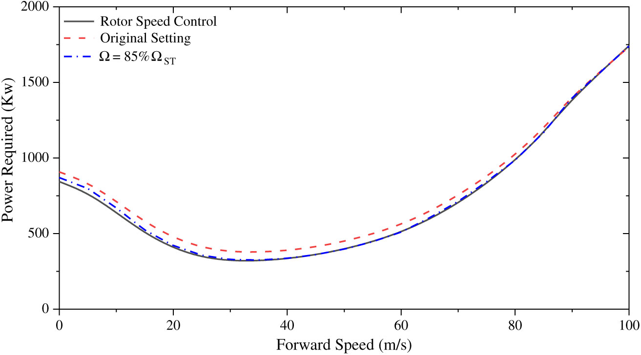
Figure 6. Power required comparison.

Although the variable rotor speed strategy could reduce the power required, the additional gearing system would increase the overall gross weight and decrease this benefit to some extent. However, these investigations still provide an additional possibility for the further improvement of the coaxial compound helicopter with LOS.

4.0 FLIGHT DYNAMICS ANALYSIS

4.1 Trim characteristics

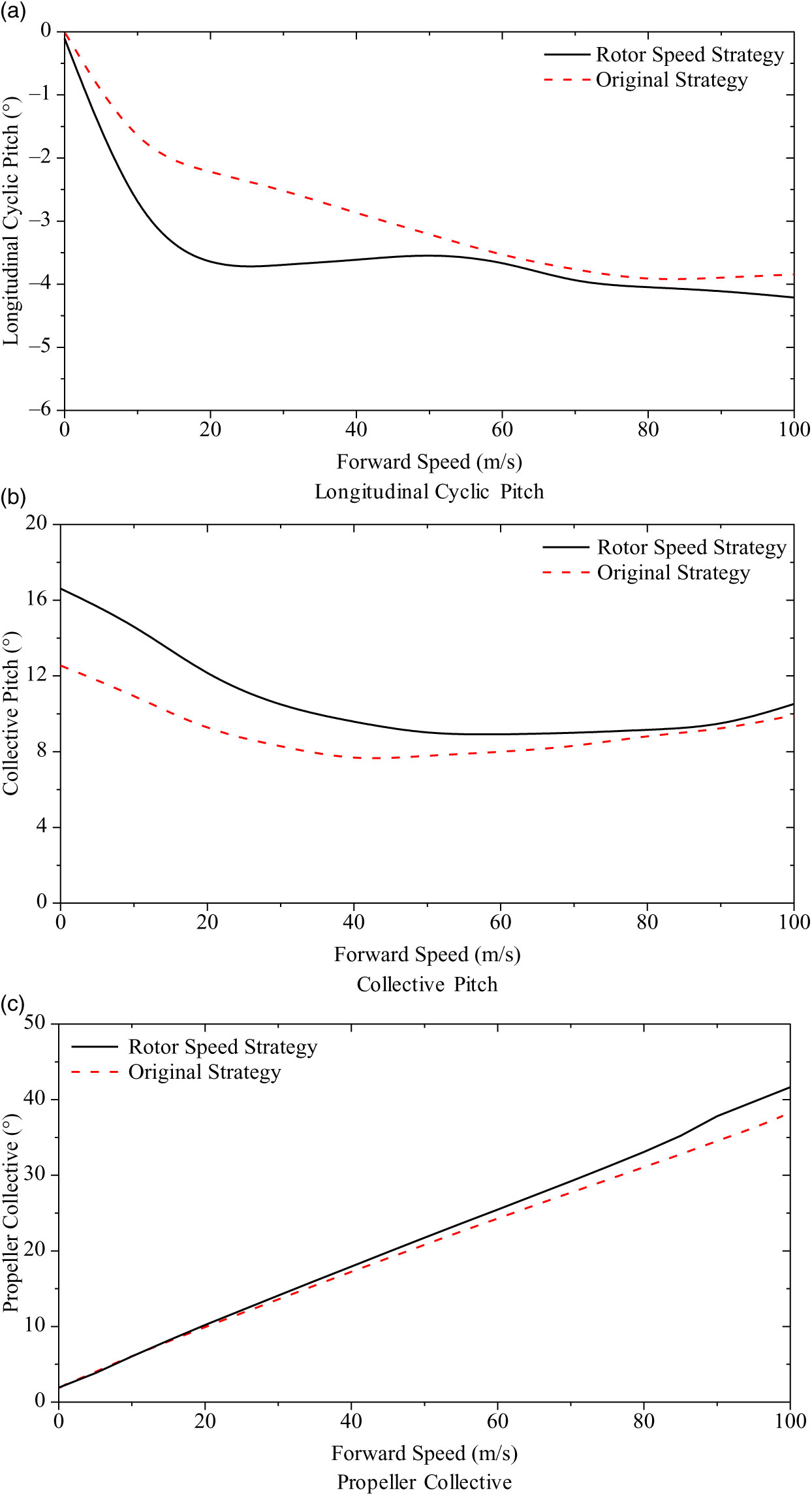
Figure 6 shows the trim characteristics with the rotor speed strategy proposed above, and the original rotor speed strategy is set as a comparison.

As demonstrated in Fig. 7, there are three differences due to the change of the rotor speed. Firstly, the collective pitch is higher across the flight range. The dynamic pressure on the rotor is lower when the strategy in Fig. 5 is adopted, which means that the extra collective pitch is needed. Secondly, the longitudinal cyclic pitch drops slightly in high-speed flight. In this flight range, the aim of the longitudinal cyclic pitch is mainly to balance the pitching moment as the forward thrust is mainly provided by the propeller. The pitching moment is composed of three parts—the wind flapping effect (nose-up moment), the control flapping effect (nose-down moment), and the moment from the fuselage and tails (nose-down moment). The decrease of the rotor speed would reduce the wind and control flapping effect proportionately if the longitudinal cyclic pitch is fixed. However, the moments from the fuselage and tails are independent from the rotor speed and the reduction of the rotor speed lowers the control power of the cyclic pitch. Thus, the longitudinal cyclic pitch should reduce slightly to keep the helicopter in balance. Meanwhile, the propeller collective results with different rotor speed strategies are similar across the flight range. The propeller collective is utilized to balance the drag of the fuselage and the coaxial rotor system. The minor change of the propeller collective with different rotor speed strategies is due to the rotor speed effect on the coaxial rotor drag. In conclusion, the rotor speed strategy has an effect on the trim characteristics. However, it does not induce any discontinuity in control inputs, which would satisfy the related requirement in handling qualities specification.

Figure 7. Trim results with the rotor speed strategy.

4.2 Longitudinal channel analysis

This article assesses the short-term response characteristics (bandwidth and phase delay), and the mid-term response characteristics (eigenvalues) with the handling qualities specification ADS-33E-PRF^{(Reference Standard34)}. In addition, to obtain the bandwidth and phase delay, the dynamic models of control mechanism and actuator are needed, this paper utilizes standard transfer functions of Eq. (16) and Eq. (17) to simulate them⁽²²⁾.

(16) \begin{equation} {\rm S}_{C{\rm ontrol}} =\frac{{\rm 16.9747}}{{\rm s}^{{\rm 2}} {\rm +44.4s+986}} \label{eqn16} \end{equation}

(17) \begin{equation} {\rm S}_{A{\rm ctuator}} =\frac{{\rm 1}}{{\rm 0.2s+1}} \label{eqn17} \end{equation}

where: ${{\rm S}_{C{\rm ontrol}} }$ is the dynamic model of the control mechanism; ${{\rm S}_{A{\rm ctuator}} }$ is the dynamic model of the actuator.

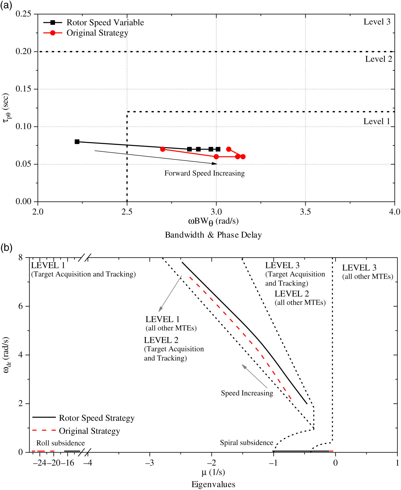
The bandwidth & phase delay and eigenvalue results in the longitudinal channel with various speeds are shown in Fig. 8, in which the results obtained by the original strategy in Fig. 2 are also added as a comparison.

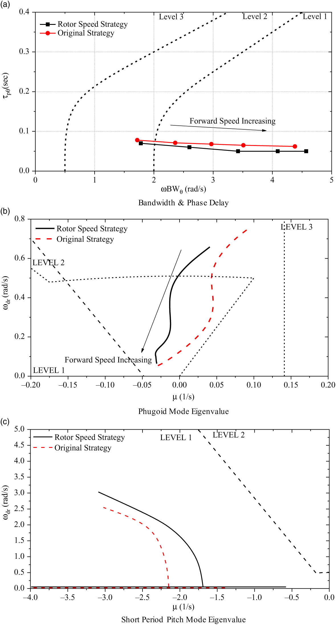
Figure 8. Longitudinal Channel Results.

As indicated in Fig. 8(a), the bandwidth increases and the phase delay drops slightly with forward speed increases. The Level 2 rating of the bandwidth and phase delay results only occurs when the forward speed is relatively low. These characteristics are similar to other helicopters⁽²⁴⁾. The eigenvalue trend demonstrates that the stability increases with speed. The longitudinal phugoid mode eigenvalue is in Level 2 in hover and low-speed flight, and the short period pitch mode eigenvalue is in Level 1 across the flight range.

The rotor speed mainly increases the value of the phase delay. As suggested by the analysis above, the decrease of the rotor speed can reduce control power and make it more difficult for the pilot to adapt the control strategy for even a small change at a relatively high frequency. Meanwhile, the rotor speed would influence the velocity and incidence stability and the pitching damping. The phugoid mode rating is better with the rotor speed strategy proposed in this article. In practice, this stability of the phugoid mode is affected by two stability derivatives, which are the velocity stability and the incidence stability. The velocity stability is usually high for the coaxial compound helicopter, as the coaxial rigid rotor provides sufficient stability across the flight range. The incidence stability of the coaxial compound helicopter is low because the rotor hub moment provides the negative incidence stability. Therefore, the reduction of the rotor speed would improve this stability because this negative incidence stability is dependent on the rotor speed. As indicated in Fig. 8(c), the rotor speed strategy also influences the longitudinal short period mode. The influence of this mode is mainly due to the rotor speed effect on the aerodynamic damping. This damping is reduced when the rotor speed is decreased, which brings about the instability to the helicopter in this mode. Despite the fact that the rotor speed strategy has a destabilizing effect on the short period mode, it still remains in the level 1 region.

It should be mentioned the results become closer at high-speed flight range as the original rotor speed strategy also drops down in high-speed flight. Overall, the proposed rotor speed strategy can still obtain effective stability and controllability in longitudinal channel.

4.3 Lateral channel analysis

Figure 9 shows the bandwidth and phase delay and the eigenvalue results in the lateral channel with variable rotor speeds. Also, the original strategy results are included as a comparison.

Figure 9. Lateral Channel Results.

As demonstrated in Fig. 9, the lateral bandwidth and phase delay results are improved with forward speed increases. The level 2 bandwidth & phase delay situation only occurs in hover and low-speed forward flight. The rotor speed influences the control power and the damping characteristics, which would change the bandwidth and phase delay results.

Both the bandwidth and phase delay are lower using the optimal rotor speed strategy due to the reduction of the control power in lateral axis. The effect of the rotor speed is more significant compared with the longitudinal axis. The reduction of the rotor speed would decrease the dihedral stability, rolling damping, and the control derivative of the lateral cyclic pitch, which degrades the results of the bandwidth and phase delay. According to the eigenvalue results, the spiral subsidence results move to the left on the complex plane (become more negative) indicating a stabilizing effect. The coaxial compound helicopter utilizes the vertical tail rather than the tail rotor to provide the heading stability, and its effectiveness is poor at the low-speed range, leading to a degraded spiral subsidence mode at this flight range. The roll subsidence eigenvalue moves to the right, which leads to an additional instability. This mode can be affected by the aerodynamic damping in rolling axis, which is dependent on the rotor speed. The decrease of the rotor speed would lead to the degradation of this mode stability. In addition, the rotor speed has a slight influence on the Dutch-roll stability, which is decreased when the rotor speed strategy is utilized. The reduction of the Dutch-roll stability is due to the rotor speed effect on the rolling damping and related stability derivatives.

Although, the rotor speed would influence the flight dynamics characteristics in the lateral channel. The rating results are still satisfied according to the handling qualities specification.

5.0 ROTOR SPEED STRATEGY IN MANEUVERAND VERTICAL CHANNEL ANALYSIS

According to the analysis above, the rotor speed strategy influences the flight dynamics characteristics. However, based on the handling qualities specification of ADS-33E-PRF, the coaxial compound helicopter with LOS rotors would still satisfy these handling qualities requirements. The investigation so far has not assessed the vertical control channel and the impact on maneuver capabilities. It was demonstrated earlier that control power can be reduced by the variable rotor speed strategy. The handling qualities in the vertical channel should be carefully assessed and the maneuver characteristics should also be involved. The rotor speed strategy should be designed to take into account the requirements of the maneuver to ensure performance is not degraded.

5.1 Rotor speed strategy in maneuver

Using the rotor speed strategy described above, there is a possibility that maneuver capability may be damaged, especially in vertical flight, therefore, a dual rotor speed strategy will be required to ensure good maneuverability. The aim of the rotor speed strategy in maneuvering flight can be divided into three aspects: the first aspect is to help the helicopter to achieve the maneuver requirements; the second aspect is to reduce the power consumption and pilot workload during the maneuver as much as possible; the third part is that it can avoid rotor dynamics problem by switching rotor rotational speed quickly.

The variable rotor speed strategy in the maneuver is set as a function of rotor normal loading ${n_{z} }$ ^(36,37). The normal load factor ${n_{z} }$ is a measure of vertical acceleration and defined as:

(18) \begin{equation} n_{z} =1-\ddot{z}/g \label{eqn18} \end{equation}

The normal load factor reflects the thrust that rotor needs to provide. The rotor speed should increase with this parameter to prevent the rotor from stalling. The proposed rotor speed strategy in maneuver can be expressed as:

(19) \begin{equation} \Omega /\Omega _{ori} =1+a(n_{z} -1) \label{eqn19} \end{equation}

where ${\Omega _{ori} }$ is the rotor speed strategy in Fig. 5. The factor a can be varied depending on the rotor aerodynamic characteristics. The main limit for the factor a is to prevent the advancing side of the rotor from experiencing compressibility effects across the flight range. This limit can be represented as follow:

(20) \begin{equation} 0.9R\{ 1+a(n_{z} -1)\} \Omega _{ori} \le (M_{critical} \cdot a_{c} -v_{\max } ) \label{eqn20} \end{equation}

where ${M_{critical} }$ is the critical Mach number of the airfoil; ${a_{c} }$ is the local sound velocity; ${v_{\max } }$ is the maximum speed for this helicopter. Firstly, the aerodynamic performance of the rotor tip is reduced due to the tip loss effect. Meanwhile, a too-large limit would weaken the maneuverability of the helicopter. Therefore, the 0.9R is set to be the reference point in this boundary condition. This setting could not only keep the most of the effective blade element away from the compressibility effect, but also guarantee the rotor performance and helicopter maneuverability across the flight range.

5.2 Pull-up & Push-over MTE

The objective of the Pull-up & Push-over MTE is to assess the handling qualities mainly in longitudinal and vertical channels. The mathematical description of this MTE has been explained widely in other literatures^{(Reference Thomson and Bradley38,Reference Thomson and Bradley39)} . Therefore, only a brief overview of this method is shown in this article.

During the Pull-up & Push-over MTE, the helicopter starts at the trimmed condition at a flight speed equal to 120kt (approximately 60m/s). Then, it is required to achieve a positive normal load factor at given time (1s for level 1) and maintain this for a given period (2s for level 1). After that, the helicopter needs to transition to obtain a negative load factor (2s for level 1) and keep this load factor for a while (2s for level 1). Finally, the helicopter should recover to level flight as quickly as possible. The glideslope angle is defined by the following equation:

(21) \begin{equation} \gamma {\rm =-}\sin ^{-1} \frac{\dot{z}}{V} \label{eqn21} \end{equation}

Combining Eq. (21) with Eq. (18), the time derivative of the glideslope angle can be expressed in terms of the normal load factor ${n_{z} }$ , which is:

(22) \begin{equation} \dot{\gamma }=\frac{\dot{V}\dot{z}-Vg(1-n_{z} )}{V^{2} \cos \gamma } \label{eqn22} \end{equation}

As mentioned above, the maximum normal load factor of this coaxial compound helicopter could achieve 2.2. Thus, the load factor distribution that relates to the level 1 standard set in the specification is shown in Fig. 10.

Figure 10. Level 1 load factor throughout the Pull-up & Push-over MTE

To represent this mathematically, the maneuver is split into six sections and fifth-order polynomials are formed to describe the load factor distribution at each section. The polynomial should guarantee the value of the load factor at every time point to satisfy the requirement and the transition between each of the sections will be smooth.

Except for the boundary condition of Eq. (22), there are three additional boundary conditions required for the helicopter. Firstly, the velocity in this MTE is assumed to be the function of the glideslope angle, which is based on the balance of energy:

(23) \begin{equation} \dot{V}{\rm =-}g\sin \gamma \label{eqn23} \end{equation}

Also, the track and heading angle should be fixed at zero during the maneuver, which formulates two boundary conditions:

(24) \begin{equation} \chi =0 \label{eqn24} \end{equation}

(25) \begin{equation} \dot{\psi }=0 \label{eqn25} \end{equation}

Equations (22–25) compose the boundary conditions of this MTE, from which it can be utilized to calculate the control inputs during the maneuver using the inverse simulation method.

5.3 Maneuver results and analysis

The control input results of this maneuver using the rotor speed strategy of Eq. (19) are shown in Fig. 11. Also, the results of the original strategy (Fig. 2) are also calculated as a comparison.

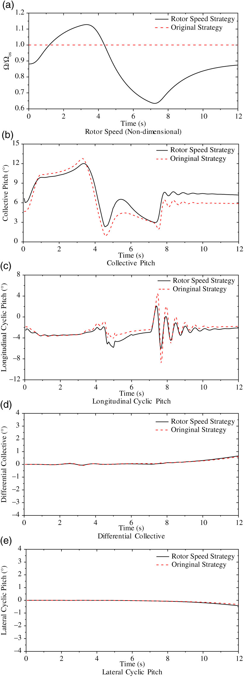
Figure 11. Control Inputs of Pull-up & Push-over MTE maneuver.

According to Fig. 11, the coaxial compound helicopter with both the rotor speed strategies could achieve this maneuver. Meanwhile, the trend of the control inputs are similar with different rotor speed strategies, which illustrates that the change of the rotor speed would not significantly influence the basic maneuver characteristics once the rotor has the capability to accomplish this MTE. Also, it is worth noting that the rotor speed response has a significant difference compared with the rotor loading setting in Fig. 10 due to the lag effect of the rotorspeed governor/engine system.

Based on the comparison in Fig. 11, there are two differences between them. First is the collective pitch. With the rotor speed variation during the maneuver, the change of the collective is much less. The change of the rotor speed variation could restrain the amplitude of the collective pitch during this maneuver. The second difference is the longitudinal cyclic pitch results during the maneuver time between 7s and 10s. At this time range, the helicopter is finishing this maneuver, and the stability of the helicopter plays a major effect. The incidence stability is relatively low for this helicopter, and the rigid rotor would aggregate this effect, which leads to the oscillation in the longitudinal cyclic pitch. On the other hand, the decrease of the rotor rotational speed would reduce the hub moment provided by the rotor, and consequently weaken this instability. Therefore, the oscillation is attenuated when the rotor speed strategy is adopted.

To assess the pilot workload of the helicopters during this maneuver, a time-domain pilot workload metric can be utilized, which is described in various articles^(40,41). The pilot workload metric includes two evaluation indices, which are the aggressiveness and the duty cycle.

Aggressiveness is a measure of control deflection magnitude from the trim control input position over the MTE, which can be defined as:

(26) \begin{equation} J_{A} =\frac{100\% }{t_{f} -t_{0} } \sum _{t=t_{0} }^{t_{f} }\left(\frac{\left|\delta (t)-\delta _{trim} \right|}{\delta _{\max } -\delta _{\min } } \right) \Delta t \label{eqn26} \end{equation}

where: ${J_{A} }$ is the aggressiveness index; ${t_{f} }$ is the MTE completion time; ${t_{0} }$ is the MTE initial time; ${\delta (t)}$ is the control inputs during MTE; ${\delta _{\max } }$ and ${\delta _{\min } }$ are the maximum and minimum control deflection respectively.

Duty cycle is a measure of the frequency of the adjustment change across the MTE maneuver, which can be calculated by the Eq. (27):

(27) \begin{equation} J_{DC} =\frac{J_{peaks} }{t_{f} -t_{0} } \label{eqn27} \end{equation}

where: ${J_{DC} }$ is the duty cycle index. ${J_{peaks} }$ is the number of the peaks during the maneuver, which is defined as a change in magnitude greater than 0.5% of the total deflection range and in the direction opposite from the previous input.

Therefore, the pilot workload metric of this maneuver can be calculated, which are shown in Table. 3.

Table 3 Pilot workload metric results

Based on Table. 3, the pilot workload is reduced when the rotor speed strategy is adopted as the change of the rotor speed would provide the additional thrust required in the maneuver. Therefore, the pilot workload is decreased. In addition, the variable rotor speed strategy could tune the control power of the cyclic pitch, and reduce the aggressiveness in longitudinal control input to a large extent.

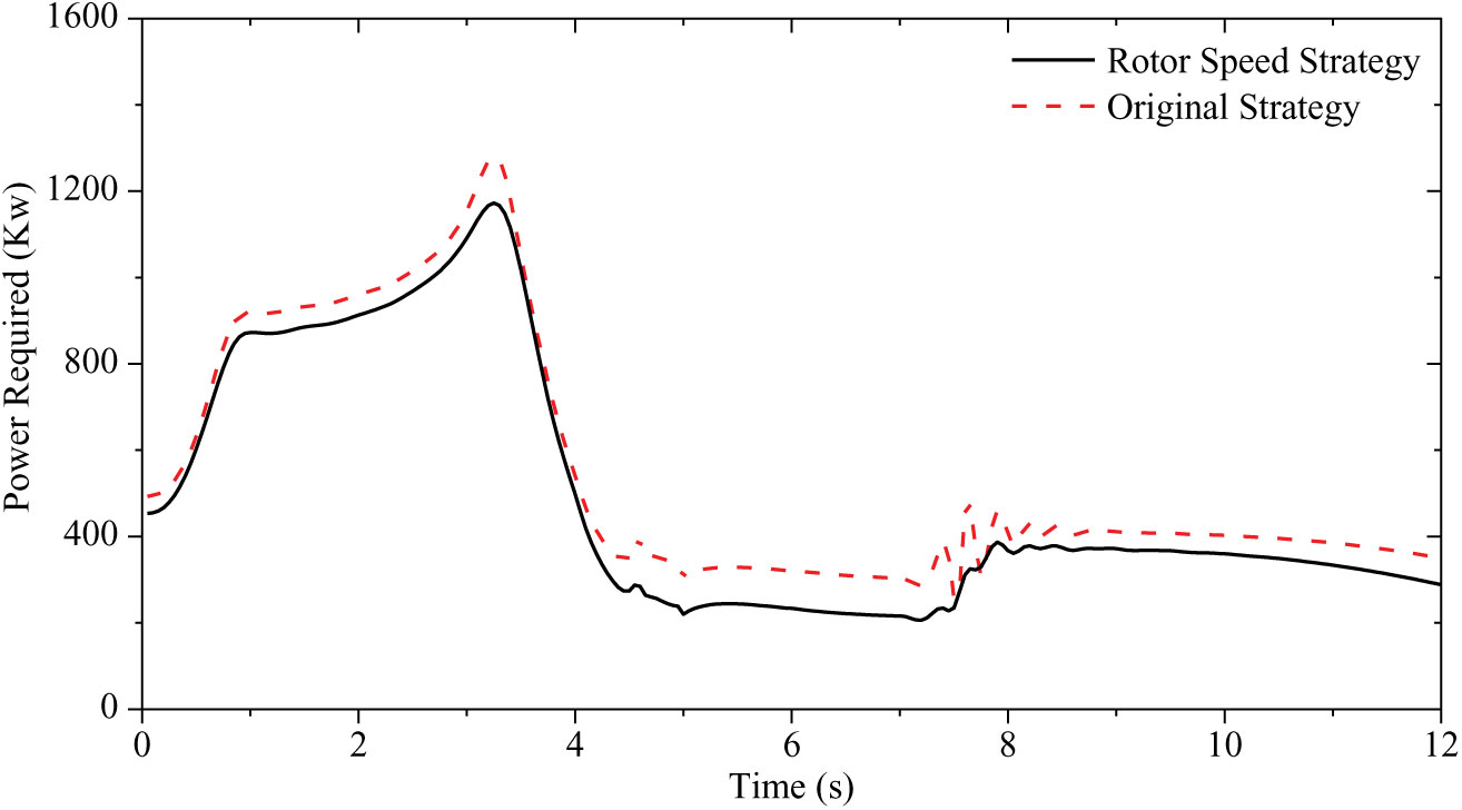
The comparison in power required with different rotor speed strategies is shown in Fig. 12, which illustrates that the rotor speed strategy could further reduce the maximum transient power consumption during the maneuver.

Figure 12. Comparison in power required with different rotor speed strategies.