2.1 Grid generation

The geometry and CAD model of the 203-mm projectile understudy is generated using Creo Parametric. The model was imported to Pointwise, a CFD meshing tool, in which surface and volume meshes were developed. Since for LES turbulence modeling, non-dimensional wall distance is required to be of the order of 1 or <1 (y + ≤1) to accurately resolve the boundary layer, hence, surface meshing and boundary-layer resolution was selected keeping in view the computational requirement. The projectile spin rate for each charge (1 – 7) was calculated from barrel-twist rate and exit velocity, which gives the non-dimensional spin rate ($ $) of 0.125, with spin rate ranging from 308 – 594 rad/sec and corresponding exit velocity from 233 – 534m/sec, respectively.

The procedure for LES analysis followed in the present study includes detailed flow analysis using steady RANS, based on which the assessment for required mesh resolution for LES analysis was carried out. Another RANS simulation on the new LES mesh was performed for further mesh adaptation at the near wall region and assessment for required temporal resolution. Synthetic turbulence needs to be superimposed on the mean flow of computational domain to introduce instantaneous velocities and to disturb the steady state pattern, for LES analysis to achieve faster statistically average-able state. For the current scale resolving simulation, precursor k-ε turbulence RANS model was used based on the previous study^{(Reference Chughtai, Masud and Akhtar16)}. In the present analysis, main emphasis remained on a well resolved near wall region rather than resolving eddies in the mean flow. The Magnus effect so generated is directly affected by wall shearing differential with respect to the AoA and spin rate and needs to be mimicked accurately. Hence Sub Grid Scale WALE model with y(+) ≤ 1 has been applied, as discussed later.

The meshing was carried out keeping in view the incompressible to supersonic nature of the flight regime, with sufficiently high Reynolds number (3.2 – 7.3 e⁻⁶) corresponding to the highly turbulent nature of the flow. Furthermore, CFL condition or courant number is kept 1 for subsonic and 0.5 or even 0.05 for initial stabilization of the numerical scheme in transonic and supersonic cases. Four x meshes for steady-state analysis were analysed based on RANS turbulent modeling (SA & k-ε) in the previous study^{(Reference Chughtai, Masud and Akhtar16)} and two x meshes analysed for the current transient analysis as tabulated in Table 2 below. Volume-grid spacing of 1.6μm is kept for the first 20 layers in volume extrusion, with a growth rate of 1.15 to achieve the final mesh for analysis. y(+) ≤ 1 is kept for the selected LES turbulent model to accurately resolve the boundary-layer for capturing the Magnus effect with max resolution of Turbulent Kinetic Energy. An estimate of integral length scale l ₀ (at which turbulent kinetic energy (TKE) peaks) was made based on precursor RANS, with the aim to resolve 70 – 80% TKE. 1^st cell height of 1.6μm was selected with 3 – 5 cells across l ₀. The anisotropic tetrahedral extruded layers (T-Rex cells) algorithm is used for sharp edges for surface meshing as well as for volume extrusion of boundary layer into an unstructured block. The T-Rex algorithm generates refined mesh in near wall region by extruding regular layers of tetrahedral from the boundaries. The mesh adapts to convex/concave regions and colliding extrusion fronts thereby generating high-quality cells. Three separate blocks were made, with a highly dense inner mesh block, to accurately capture shock effect and near-wall disturbance/eddies. An outer less-dense, structured rectangular block was used capturing the wake. Pictorial views of the mesh are depicted from Figs. 1–4.

Table 2 Mesh used for grid independence study

M-Meters

Mn-Million

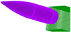
Figure 1. Surface mesh with structured wake block.

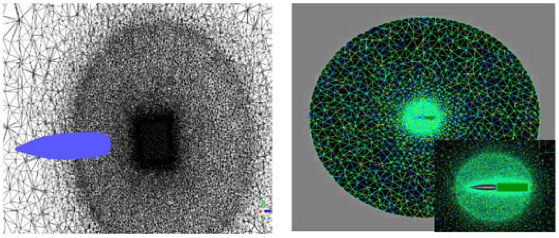
Figure 2. Volume mesh with unstructured dense inner circle.

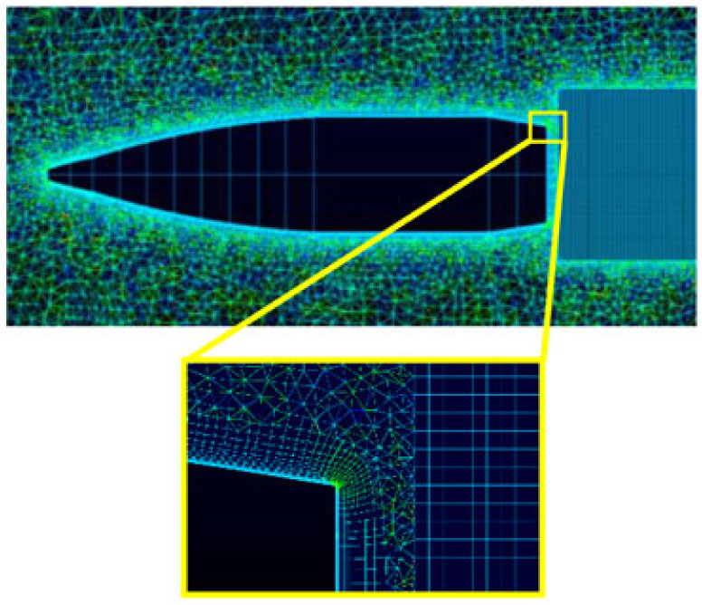
Figure 3. Boundary layer enlarged view.

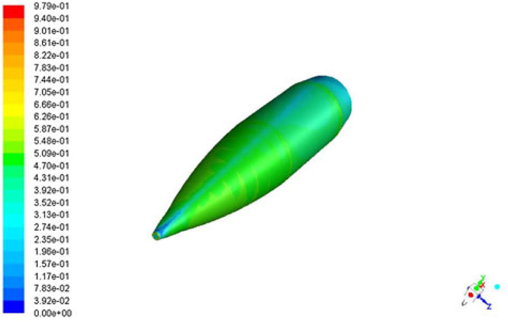
Figure 4. Y Plus distribution on projectile surface at Mach 0.7.

2.2 Grid optimization

Two meshes, with sufficiently fine surface mesh and boundary-layer extrusion with T-Rex cell (anisotropic tetrahedral extrusion), were developed to study grid independence (mesh 5 and 6, respectively) and were validated against available experimental data of the drag coefficient from Mach 0.7 to Mach 1.6 at zero AoA and Magnus force coefficient for Mach 0.7. Both meshes were found to predict with reasonable accuracy (<5% deviation from experimental drag-coefficient calculation^{(Reference Dickinson8)}), hence, no further mesh was analysed. Being computationally economical, mesh #5 was selected for subsequent analysis. It has been found that steady-state (SS) analysis with k-ε turbulence model predicts the drag coefficient in close agreement with experimental data as compared to time-accurate analysis with LES at subsonic speed. However, at transonic and supersonic speed, time-accurate LES models provide much more accurate predictions. The Table 2 shows various meshes used for the current series of analyses. Drag coefficient, predicted with SS analysis (mesh #4)^{(Reference Chughtai, Masud and Akhtar16)}, transient (mesh #5) and experimental testing at zero AoA, is compared below (Fig. 5).

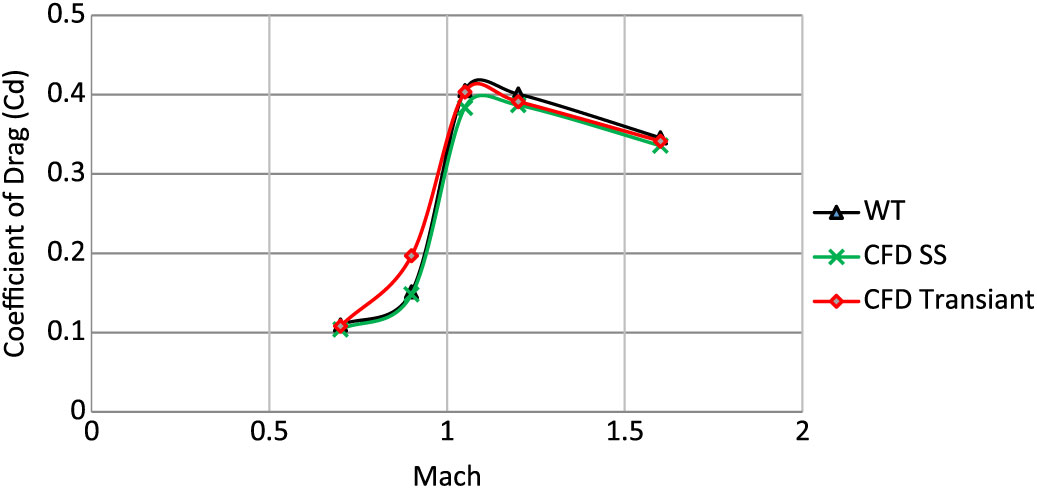
Figure 5. Drag coefficient comparison- validation of computational model.

Comparison of the drag coefficient (Cd) and Magnus force coefficient (Cyρ_α), with selected mesh as per grid independence investigation extracted from experimental^{(Reference Lieske7,Reference Dickinson8)} and numerical analysis (SS and transient – LES), is shown in Figs. 5 and 6, respectively. Notably, the experimental Magnus force coefficient, as referred to in Ref 7, was calculated based on reversed interpolation with modified point-mass trajectory model, while adjusting the form factor to match the experimental range-firing impact point and time-of-flight data. Robert. F. Lieske’s^{(Reference Lieske7)} experimental calculation of Magnus force coefficient (Cyρ_α = 0.38) was found to accurately predict the Magnus effect at subsonic mach speeds. Keeping in view the limitation of available experimental results, subsonic comparison of numerical analysis versus experimental data of Cyρ_α is considered for the current study and found to be in reasonable agreement for validation of the numerical scheme under study, as shown in Fig. 6.

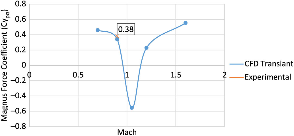
Figure 6. Magnus force (Cy_ρα) comparison – validation of computational model.

2.3 Time independence study

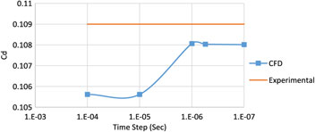
The spatial and time domains are both interrelated in an accurate capturing of pressure and viscous effects. The time step and mesh fineness needs to be small enough for precise capturing of small eddies, generated as a byproduct of complex turbulent flow. Balance needs to be maintained, both for mesh fineness and time stepping, for the problem to be computationally economical. Since transient analysis is required to capture the Magnus effects, LES model that is selected requires Y+ value of the order of 1. For such a fine boundary layer (ΔS = 1.6e-6m), the time step needs to be adjusted accordingly. As per CFL criteria, the ideal time step for the courant number of 1 in the entire Mach scheme is selected. Four time steps have been analysed at Mach 0.7 and 500 rad/sec rotational spin rate at 0° AoA, as plotted below (Fig. 7) and compared with the experimental results^{(Reference Dickinson8)}. It has been found that drag coefficient Cd remains reasonable accurate for all the time steps that have been compared and is found to be in best agreement at a time step of O e⁻⁵. However, for CFL criteria of courant number of <1 and Y+ of the order of 1 (for LES transient analysis), the time step needs to be refined to the order of e⁻⁶. Hence, in addition to Cd, Cyρ_α validation has also been considered for validation of solution model. Cyρ_α is calculated with time step of O e⁻⁶ and found to be in agreement with the experimental results (Fig. 6).

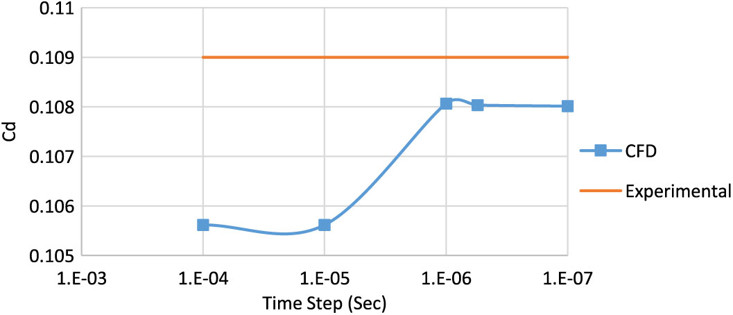
Figure 7. Drag coefficient variation with time step refinement at M 0.7, spin rate 500rad/s.

Figure 8. (a): Resolved spectrum – projectile surface. (b): Resolved spectrum – computational domain.

4.1 Flow field

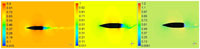
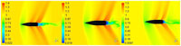
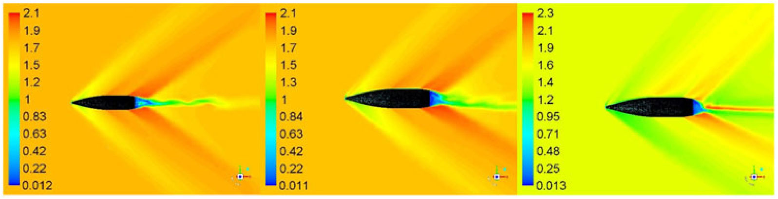
Trajectory simulations of the projectile under study necessitate generation of an aerodynamic coefficients library encompassing the complete flight envelop. Apropos, 30 cases were simulated from Mach 0.7 – 1.6 at 0, 5 and 10 degs AoA and at 500 – 750 rad/s of spin rate, respectively. Each simulation was run to allow the projectile to complete a minimum two rotations (with flow time of approximately 0.024 sec). Keeping in view the periodic boundary condition (with rotation about z-axis simulating the desired spin rate), we observed the quasi steady behavior in the desired coefficient’s plots, after one complete rotation (0.012 sec), as depicted in the lift and drag coefficients plots in Fig. 12 below. However, to ensure that the flow field to be fully developed, each case was further run for T > 0.024 sec. Mach flow field with cross-sectional planner view at Mach 0.7, 1.05 and 1.6 and at 0, 5 and 10 degs AoA at constant time interval is shown in Figs. 9, 10 and 11, respectively. The velocity variation/generation of shock wave at supersonic mach speed and fluctuating flow/vortices in wake region at subsonic speed indicates a fully developed flow. The vortex shedding with circulatory flow field (as discussed later in vortex core section) affects the upstream flow (more pronounced in subsonic/transonic flow), and results in pressure/forces fluctuation with respect to time. The effect is visible on time-history plot of Lift (Cl) and Side Force Coefficient (Cs), as plotted in Fig. 12.

Figure 9. Velocity flow field at M 0.7, AOA 0, 5, 10 (left to right) at time 0.024 sec.

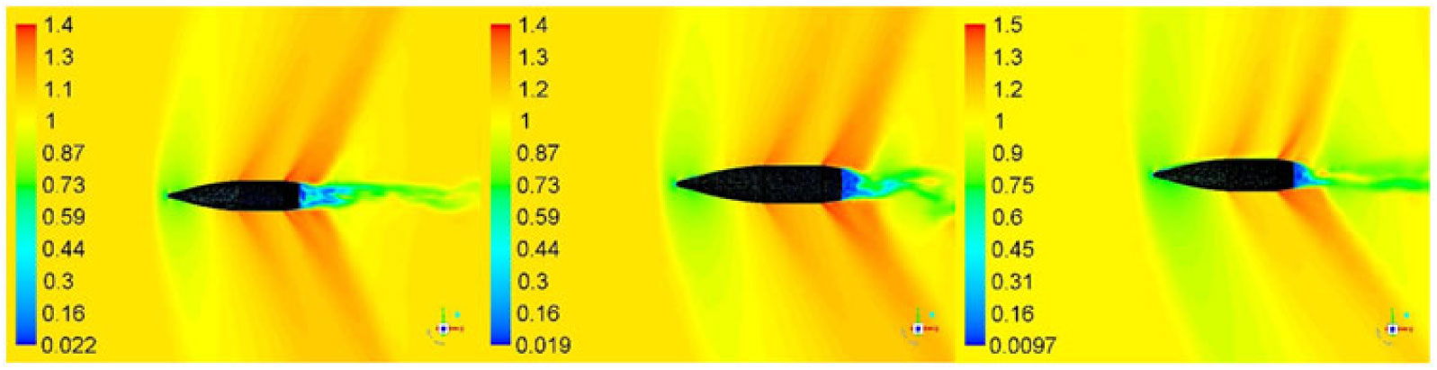
Figure 10. Velocity flow field at M 1.05, AOA 0, 5, 10 (left to right) at time 0.026 sec.

Figure 11. Velocity flow field at M 1.6, AOA 0, 5, 10 (left to right) at time 0.024 sec.

Figure 12. Convergence history of lift and yaw force coefficient (M 1.05, AOA 10 degs, 750 rad/s).

A comparison of Mach contour indicates that the flow field depends highly on upstream velocity, geometry of the projectile and AoA. The developed shock wave at Mach 1.6 (Fig. 11) shows a clear decrease in velocity once the flow encounters the shock, whereas at the mid-section and the boat-tail an expansion wave is developed with a marked increase in velocity. As apparent, the velocity field behind the boat-tail portion is very low as compared to the freestream velocity. This wake region, with circulating flow due to the blunt-shaped boat-tail portion of the projectile, generates negative pressure, and is the main contributor of drag in addition to wave, form and skin-friction drags. This is a design constraint and cannot be easily avoided, as the projectile base needs to bear the high pressure generated due to rapidly expanding propellant gases in the firing chamber.

Furthermore, there is a link between the fluctuating flow field at different Mach speeds/orientations and the dynamic behavior of the projectile during flight. An investigation was carried out to derive the correlation of Strouhal number with projectile stability by filtering the dominant frequencies from the lift and yaw force convergence histories. At each time step, the solution is fully converged and the fluctuations are well known to be attributed to vortex shedding and non-symmetric wake behavior, which eventually affects the upstream flow, thereby, disturbing the pressure distribution on the projectile surface.

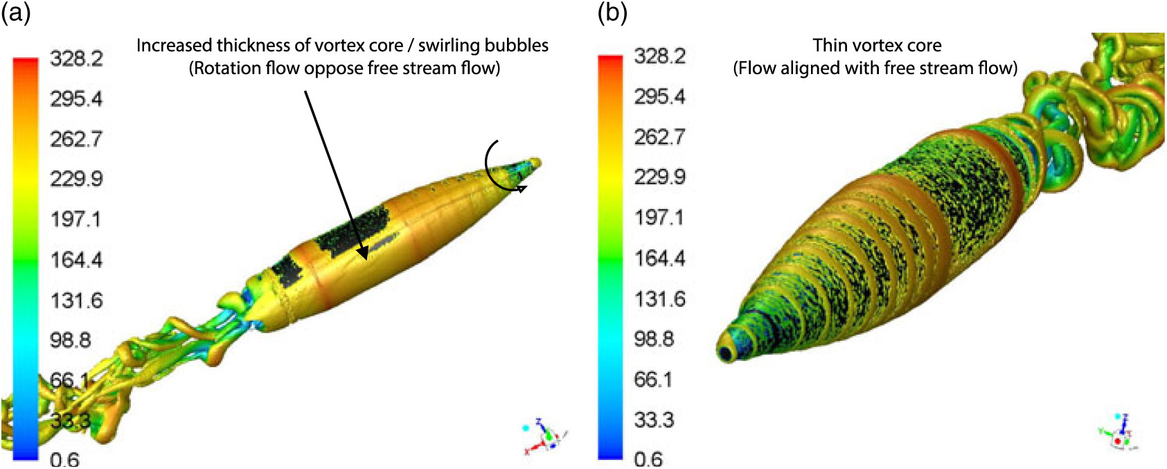
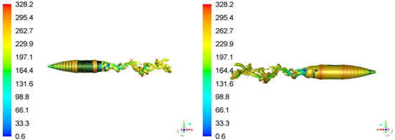
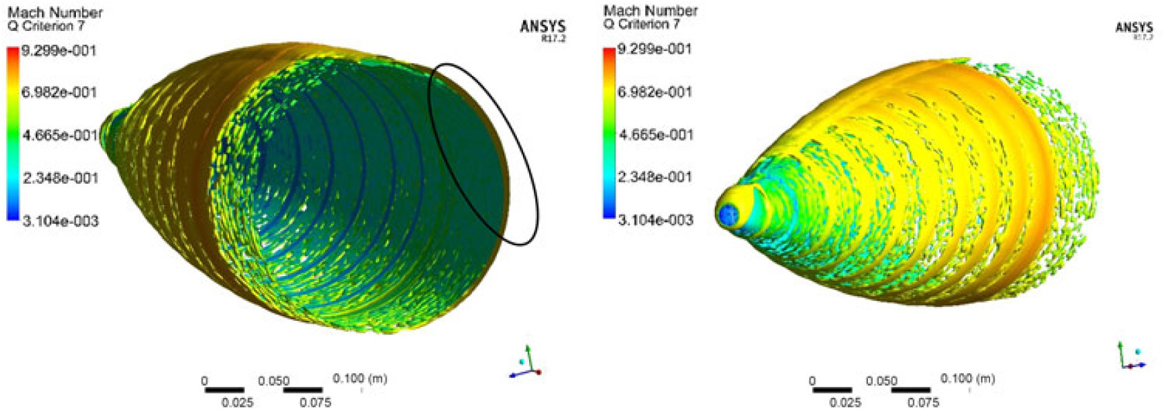
4.2 Vortex core visualization

To study the opposing flow-field interaction at AoA > 0 deg, the vortex core was plotted with Q-Criterion at Mach 0.7 at 5 degs AoA with 500 and 750 rad/s spin rates, respectively. Q-Criterion is one of the best ways to visualise the turbulent vortical structures, which uses the second invariant of the velocity gradient tensor. Once freestream velocity interacts with surface attached flow swirling with the wall, vortices with circular or spiral set of streamlines are generated. The vortex core with the definition area selected as the projectile is plotted with velocity magnitude variation, which shows the isosurface of vorticity vector on the surface. As evident, the vortex core has increased thickness on +Z-axis face of the projectile where the flow opposes the freestream flow (Figs. 13 and 14) as compared to −Z-axis view where the flow is aligned. This one-sided, wall-attached swirling flow can be observed with the cross-sectional view (at X 0.65 m) with increased thickness of the core, as shown in Fig. 15. The swirling flow, due to flow interaction, will result in surface pressure and shear stress differential resulting in generation of a Magnus force. It is a function of spin rate, AoA and Mach speed and results in variation of the Magnus force, and moment coefficient at subsonic, transonic and supersonic flow (discussed later in coefficient extraction section).

Figure 13. Vortex core (Q-criterion) at M 0.7, AOA 5 degs at 500 rad/s spin rate a T 0.026 sec. a)+Z Axis, b)−Z Axis View.

Figure 14. Vortex core (Q-criterion) at M 0.7, AOA 5 degs at 750 rad/s spin rate at T 0.026 sec.

Figure 15. Cross-sectional view of core thickness at (X = 0.65 m from nose) at M 0.7, AOA 5 degs at 500 rad/s at T 0.028 sec.

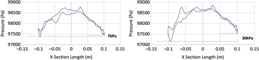
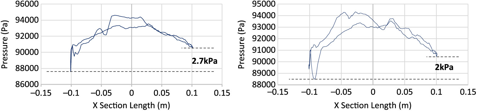
4.3 Magnus-induced cross-sectional pressure variation

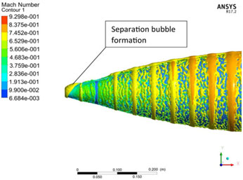
To further understand the effect of swirling flow/ripples development due to Magnus effect, surface pressure was plotted at projectile cross section (x = 0.65 m) with different Mach speed and spin rates, as shown in Figs. 16, 17 and 18, respectively. With increasing speed, the pressure differential also increases in conjunction with the increase in AoA and spin rate. The area under the curve analogy shows that the left portion of projectile (as viewed from nose) encounters greater surface pressure as compared to the other half. However, the difference in peak pressure across the projectile increases with spin rate at subsonic speed, whereas it remains negligible at transonic and supersonic speeds. Furthermore, at transonic speed, sudden spikes in the pressure curve are also observed, probably because of the isolated-flow separation bubbles generated due to opposing flows. At transonic speed, Magnus forces and moment coefficient shows inverse behavior as compared to subsonic and supersonic flows behavior, as evident from the coefficient plots.

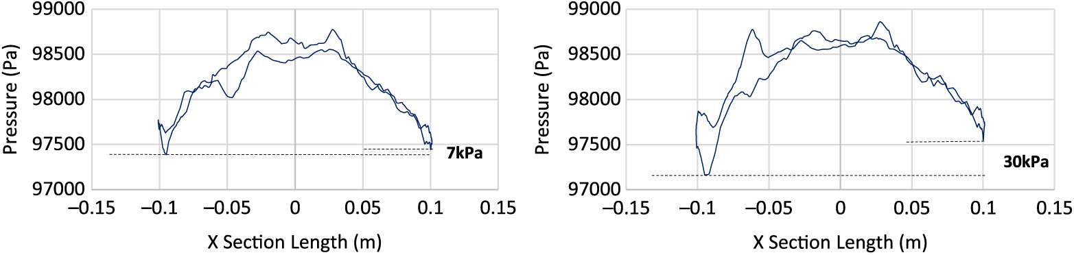
Figure 16. Surface pressure plot at X Sec 0.65 m from nose at M 0.7, AOA 5 degs at 500 rad/s (left) & 750 rad/s (right).

Figure 17. Surface pressure plot at M 1.05, AOA 5 degs at 500 rad/s (left) & 750 rad/s (right).

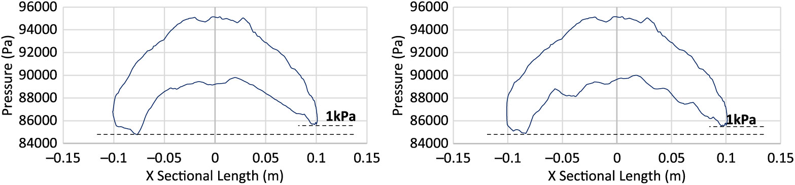
Figure 18. Surface pressure plot at M 1.6, AOA 5 degs at 500 rad/s (left) & 750 rad/s (right).

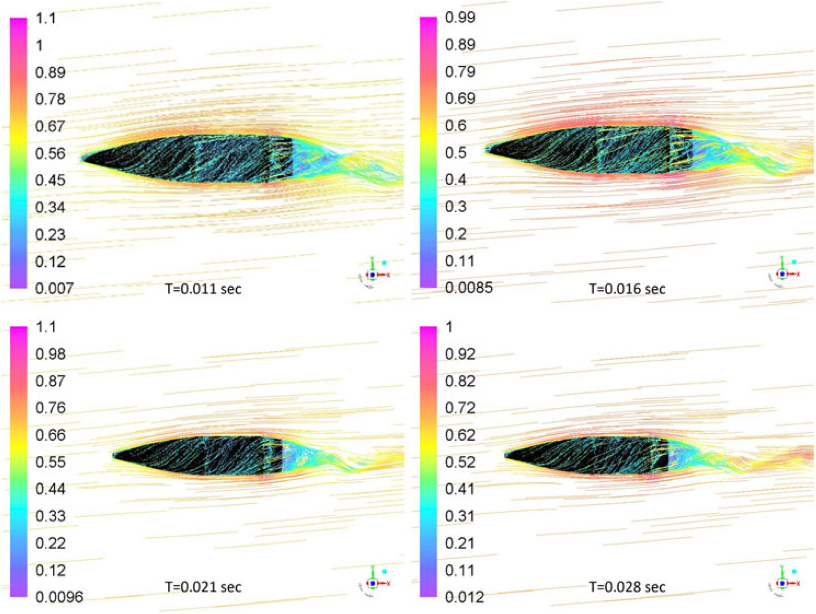
4.4 Wake flow and pathline visualization with respect to flow time

Fully developed flow at subsonic speed was analysed with Mach contour plot at various time intervals to visualise the wake flapping and vortex shedding. The shedding of vortices has its effects on upstream flow causing a significant fluctuation in lift-coefficient convergence with respect to flow time, as is also evident from the lift-convergence plot in Fig. 12. However, the shedding frequency may not be identical to vortex shedding from the cylindrical body with infinite length, at low Reynolds number, due to superimposed swirling motion caused by projectile spin, geometry edges and orientation of the projectile. Intuitively, spin imparts more inertia to the shedding vortices in addition to velocity distribution on Y and X axis, causing late detachment and subsequently, reduced shedding frequency. Likewise, the pathline plot shows adequate flow wrapping due to no-slip boundary condition and spinning of projectile. The spin also causes the swirling wake flow, as shown in Fig. 19. The pathlines show separation over the main body and boat-tail edges where the local velocity increases due to generation of an expansion wave, as shown in Fig. 20.

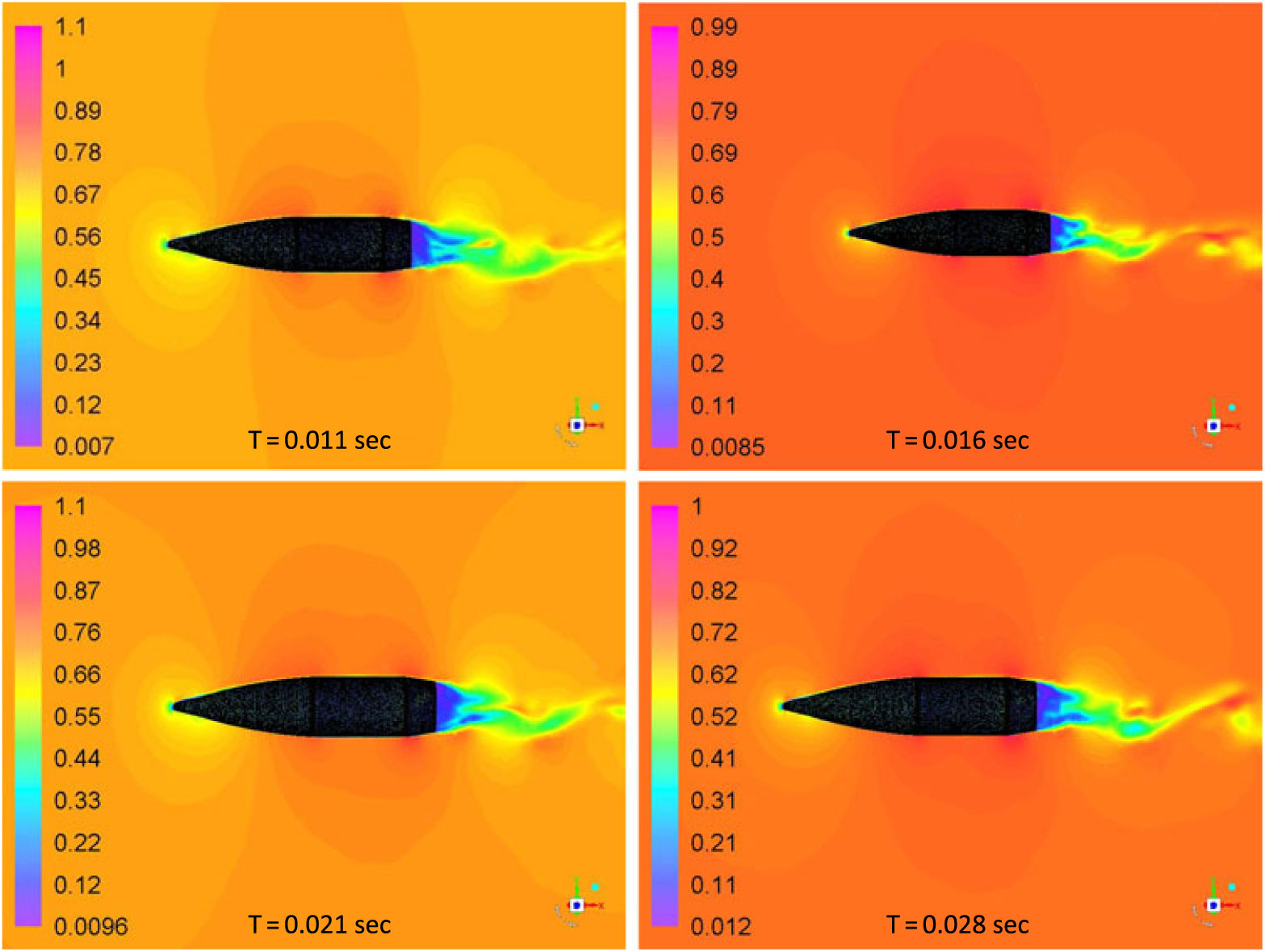
Figure 19. Mach countour plot at various time intervals: M 0.7 at 5 degs AOA, 750 rad/sec spin rate.

Figure 20. Pathlines Mach plot at various time intervals: M 0.7 at 5 degs AOA, 750 rad/sec spin rate.

4.5 Strouhal number estimation and dependence on aerodynamic loading

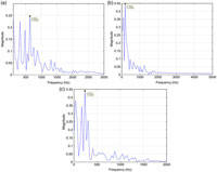
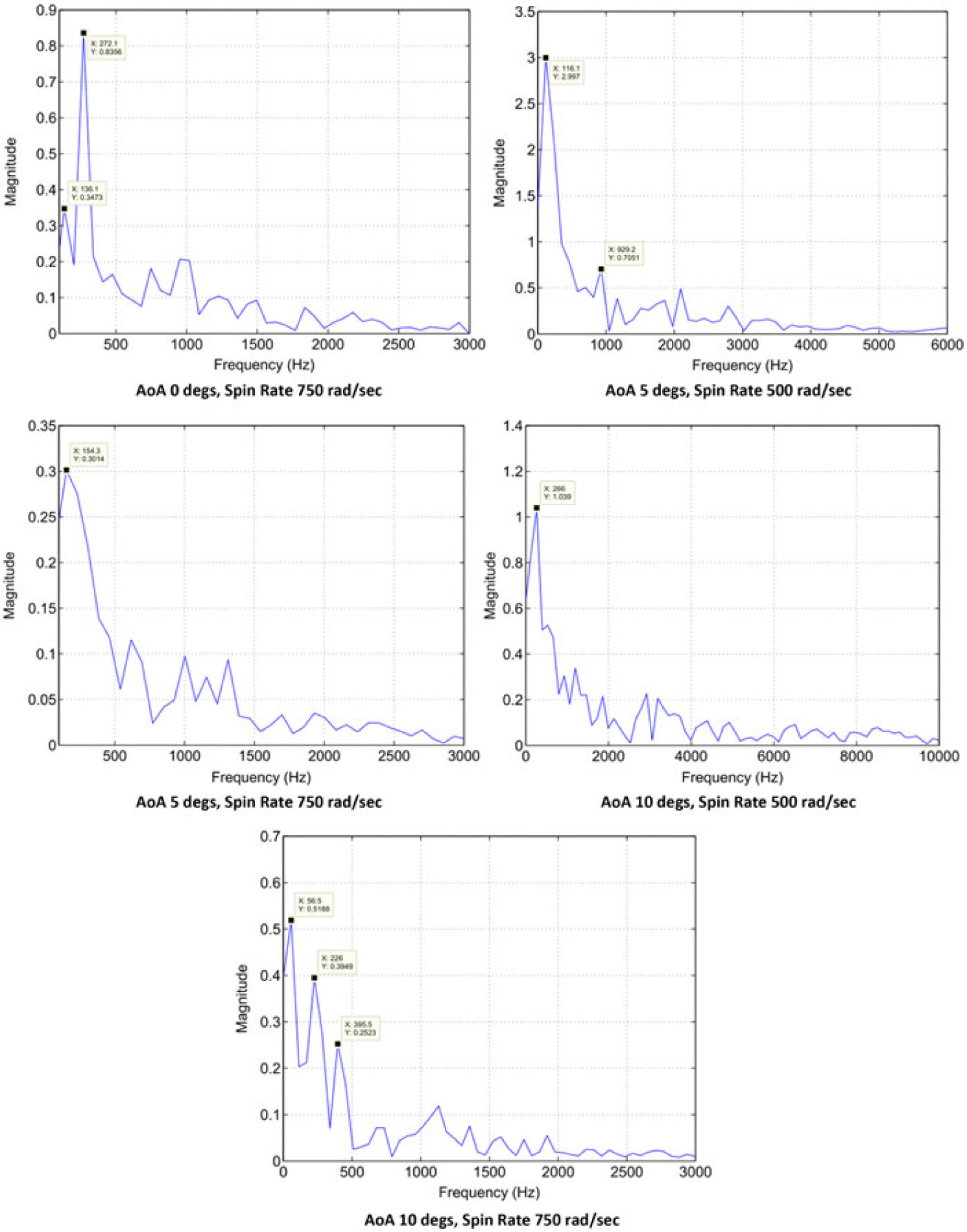
Vortex shedding frequencies at different Mach and spin rates were calculated with the analogy of finding maximum frequency component within the oscillation of lift and yaw-force convergence with respect to time. The dominant frequency corresponds to the vortex shedding frequency, particularly at low Mach speed obtained with FFT analysis. At transonic and supersonic speeds, multiple dominant frequencies were observed, which corresponds to multiple vortex shedding as evident from the flow visualization. It is found that both AoA and Mach speed have a direct effect on vortices generation and subsequent variation in lift. The FFT analysis of lift and side forces fluctuation with respect to time at Mach 0.7 is shown in Figs. 21 and 22, respectively.

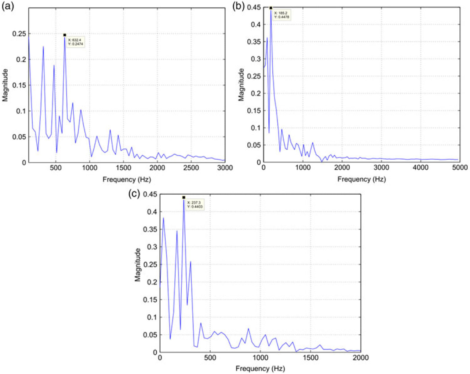
Figure 21. Lift Coefficient convergence FFT plot; M 0.7 AOA, 750 rad/sec spin rate. a) AoA 0 deg. b) AoA 5 degs. c) AoA 10 degs.

Figure 22. Side force coefficient convergence FFT plots at M 0.7.

The Strouhal umber, St($ $) calculated from the lift coefficient fluctuation history (considering the dominant frequency only) directly increases with the increase in projectile AoA at 500 rad/s however as the spin rate increases to 750 rad/s, the St shows inverse behavior. Whereas, for side-force coefficient analysis, the Strouhal number increases with the increase in spin rate at low AoA and decreases at higher AoA. The phenomenon can be explained with the help of the FFT plots, in which at higher AoA, multiple dominant frequencies were observed, as depicted in Figs. 21 and 22, respectively. The presence of multiple frequencies corresponds to multiple vortices. At higher AoA, leading-edge separation bubble interaction with trailing-edge vortices shedding, flow encountering large cross sectional area, coupled with swirling action due to spin, leads to generation of complex flow (Fig. 23), as evident from FFT analysis as well. Furthermore, the Strouhal number behavior for side force coefficient differs from lift force at higher AoA/spin rate, and may be attributed to Magnus force effect (results tabulated in Table 3). As depicted in Figs. 13 and 14, the vortex core bubbles appear due to Magnus force with opposite flow interaction and corresponding pressure differential leading to generation of side force. As the Magnus force increases with the increase in AoA, the unsymmetrical flow develops in interaction with the free stream flow leading to generation of turbulence. Hence, Strouhal number shows different behavior for side force as compared to lift-force coefficient.

Table 3 Strouhal Number (St) at Mach 0.7

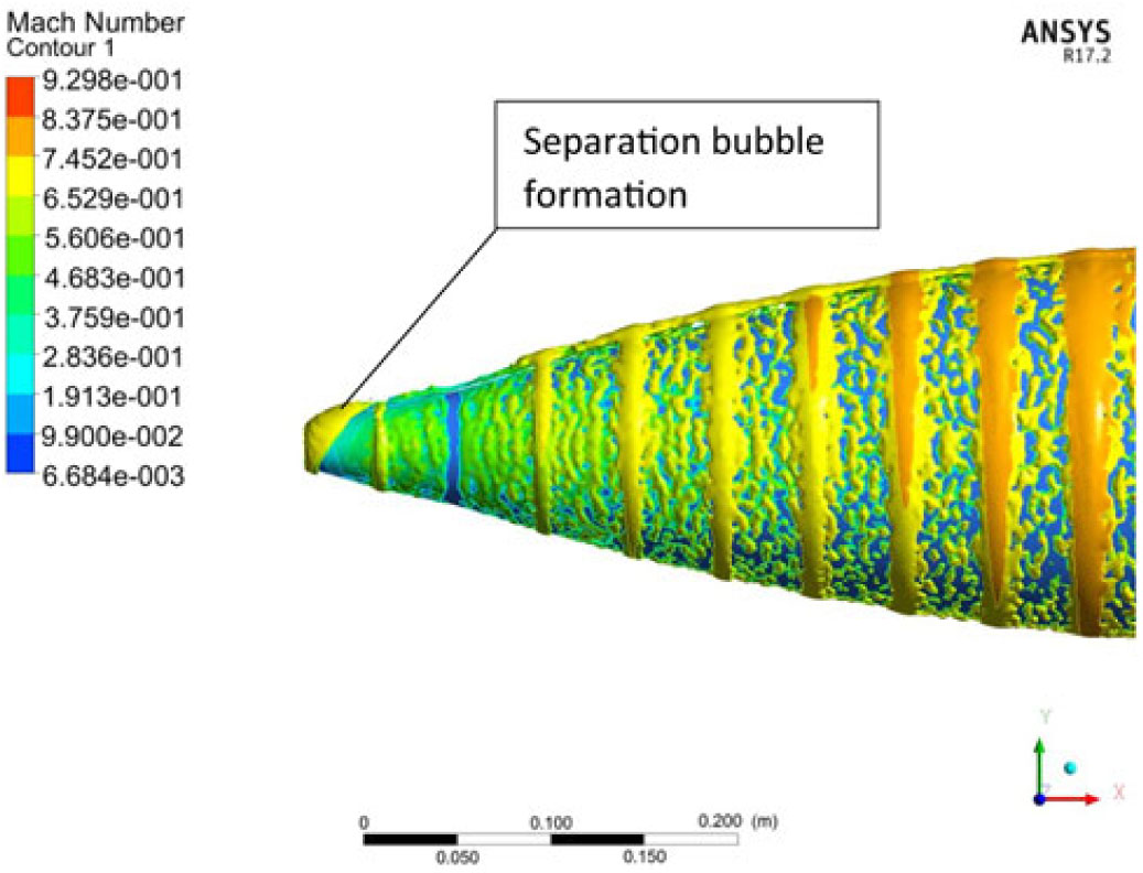
Figure 23. Leading-edge separation bubble and Magnus force induce ripples at M 0.7, AoA 10 degs at 750 rad/sec.

4.6 Static/Dynamic coefficient extraction for 6 DoF trajectory analysis

The aerodynamic coefficient library is calculated for generation of in-flight aerodynamic forces and moment for 6-DOF trajectory solver. In the previous study^{(Reference Chughtai, Masud and Akhtar16)}, the coefficients were calculated with steady-state analysis and have produced reasonably accurate results when imbedded in 6-DOF motion solver, and the simulated trajectory results were compared with the experimental data. However, the Magnus force and moment coefficient effects were not incorporated and therefore their exits a need to analyse their effect on the trajectory and dynamic stability. Hence, a time-dependent numerical analysis of projectile under study is analysed for Mach 0.7 to 1.6 for 0, 5 and 10 degs AoA, each at spin rate of 500 and 750 rad/sec. Curve-fitting methodology is then used to populate the results for further use in a 6-DOF solver. The calculated coefficients are plotted below from Figs. 24–27.

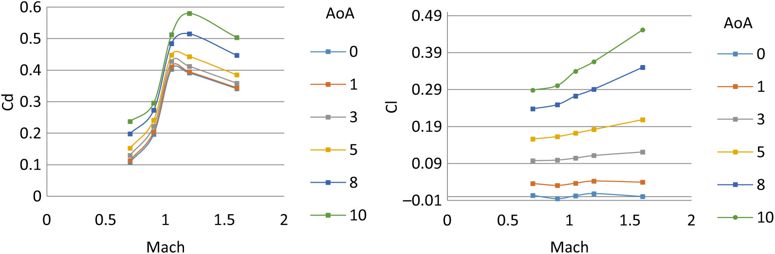
Figure 24. Drag coefficient w.r.t. AOA α (Left) – lift coefficient w.r.t. AOA α (right) at Mach 0.7–1.6.

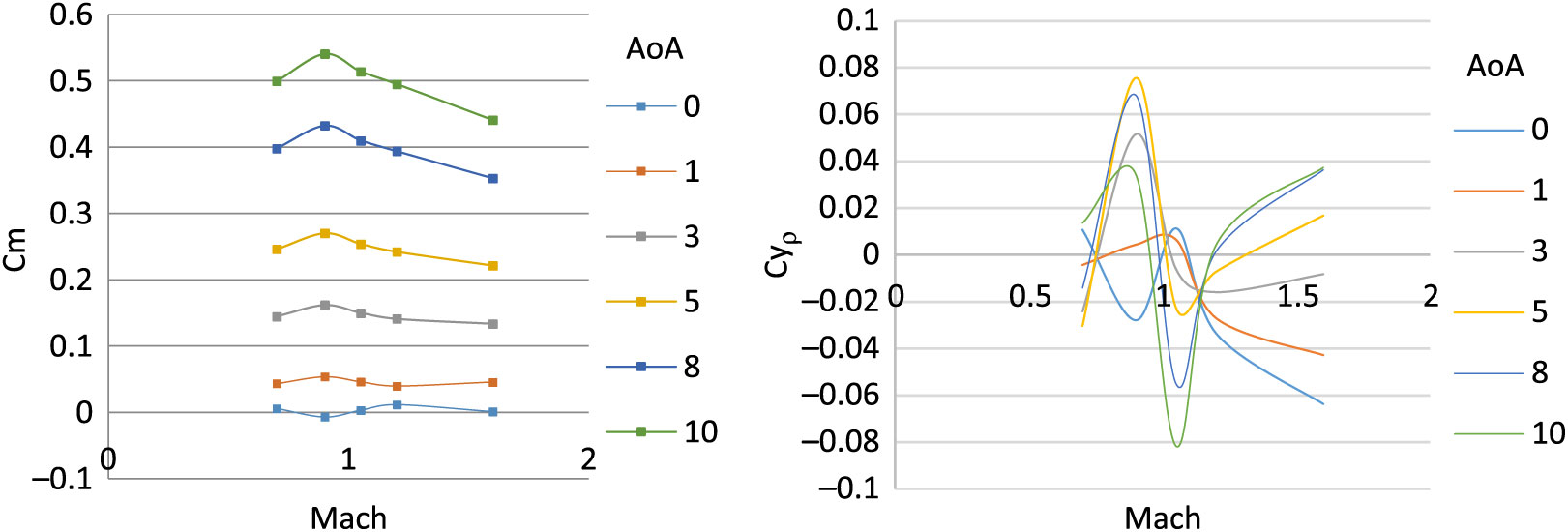
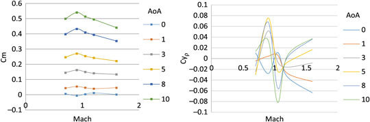
Figure 25. Pitching moment coefficient w.r.t. AOA α (left) – Magnus force coefficient w.r.t. AOA α (right) at Mach 0.7–1.6.

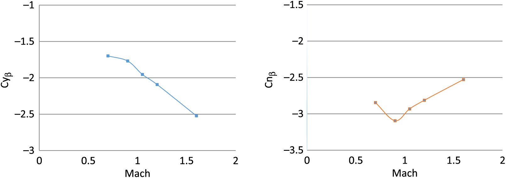
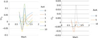
Figure 26. Side force due to sideslip angle (left) – yaw stiffness (right) at Mach 0.7–1.6.

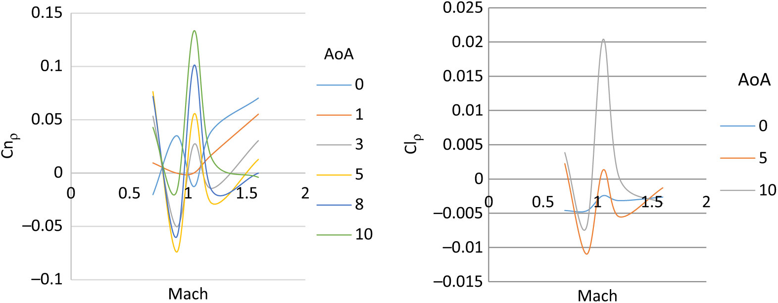
Figure 27. Magnus moment coefficient (left) – roll damping coefficient (right) at Mach 0.7–1.6.

The steady and dynamic longitudinal/lateral directional coefficients computed were found to have strong dependence on AoA (α) and sideslip angle (β) with respect to Mach speed as the changing parameter. The static coefficients remained in agreement with the steady-state analysis results with reasonable accuracy. However, the dynamic derivatives extracted from transient simulations show variation in Magnus force (Cy_ρ), Magnus moment (Cn_ρ) and roll-damping (Cl_ρ) coefficients. At transonic speed, the dynamic derivatives show abrupt, varying behavior as compared to subsonic and supersonic speed results. The same trend of Magnus force coefficient variation at transonic speed has been observed in experimental testing of 8-inch M650 spinning projectile conducted by U.S. Army Ballistic Research Laboratory for incorporation of Magnus force in modified point-mass trajectory model^{(Reference Lieske7)}.

5.1 Trajectory validation with experimental results

As for the steady-state analysis, the trajectory simulated results, based on unsteady numerical calculation of aerodynamic coefficients, are found to be in agreement with the experimental data/firing-table results. However, due to incorporation of Magnus force/moment and time-dependent effects, variation is observed in the dynamic stability of the projectile, particularly at higher Mach speed and AoA. The 6-DOF nonlinear projectile trajectory prediction mathematical model, based on flat-Earth equation of motion, is the same as used by the authors’ in the previous study^{(Reference Chughtai, Masud and Akhtar16,Reference Wessam21)} . After incorporating the revised dynamic coefficients library (as graphically depicted in Figs. 24–27 above) in 6-DOF trajectory solver, the computed flight parameters were calculated, as plotted from Figs. 28–31.

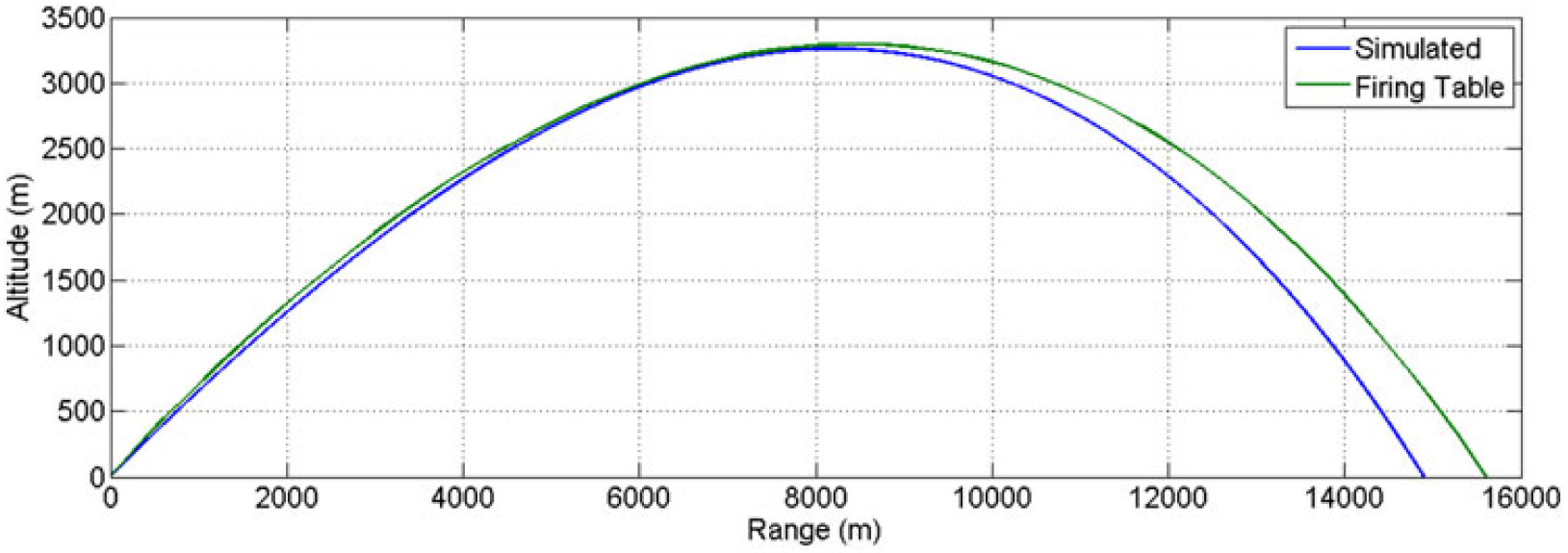
Figure 28. Trajectory plot at charge 7 (MV 595 m/sec) at 600 mils.

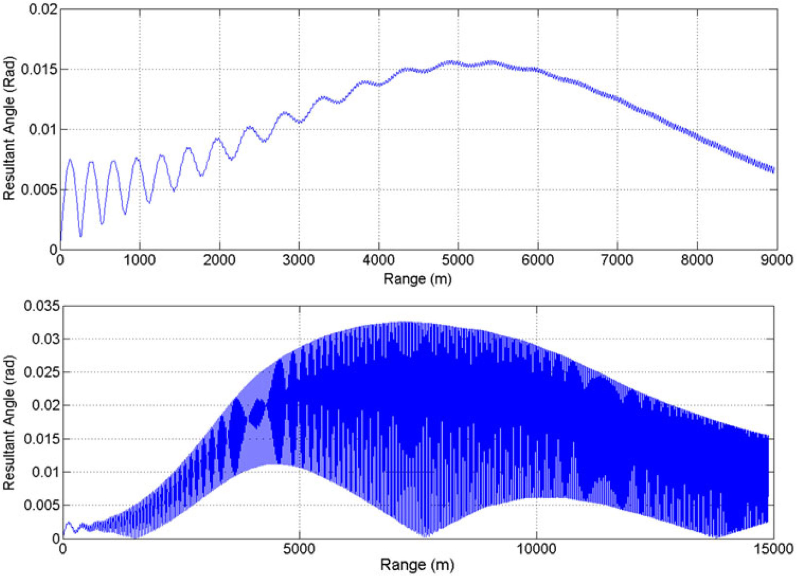
Figure 29. Resultant aerodynamic angle (rad) vs range, charge 4 (MV 350 m/sec) (above) – charge 7 (MV 595 m/sec) (below) at 600 mils.

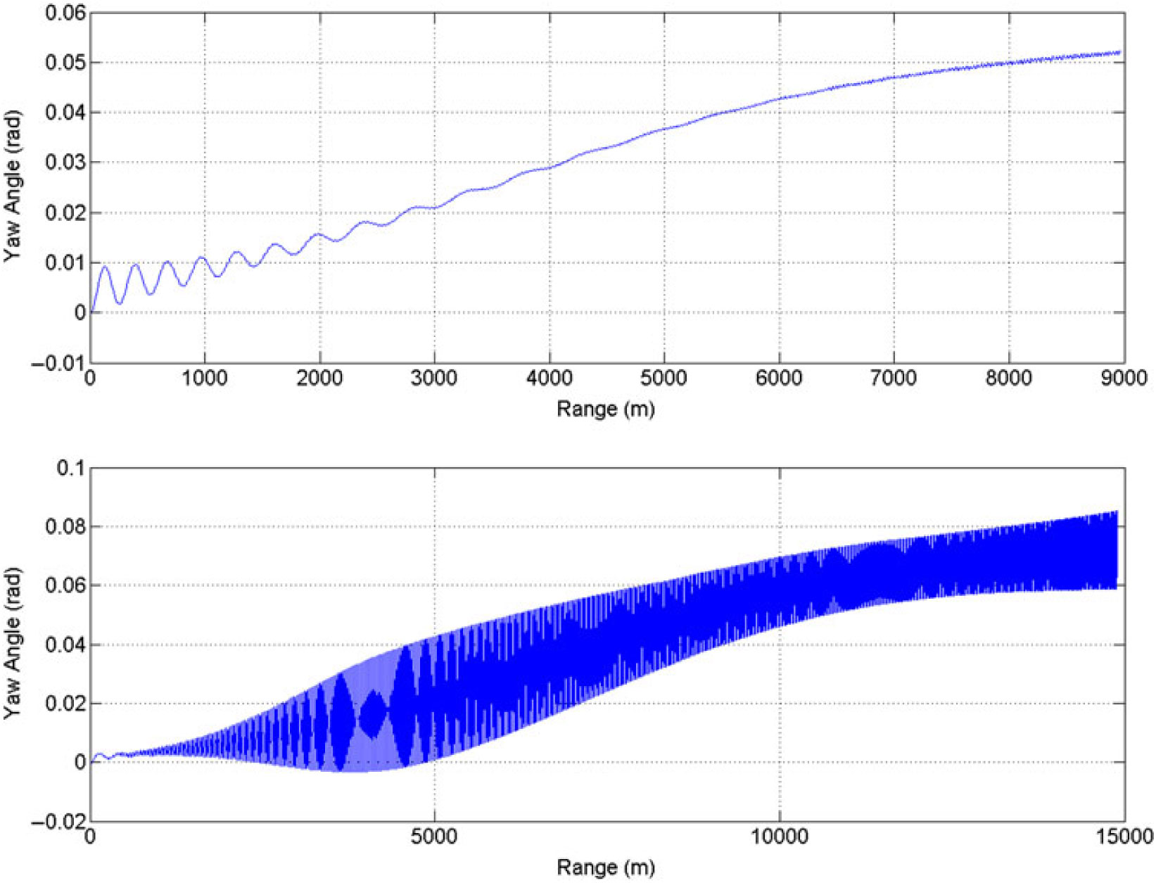
Figure 30. ψ vs range (equilibrium yaw), charge 4 (MV 350 m/sec) (above) – charge 7 (MV 595 m/sec) (below) at 600 mils.

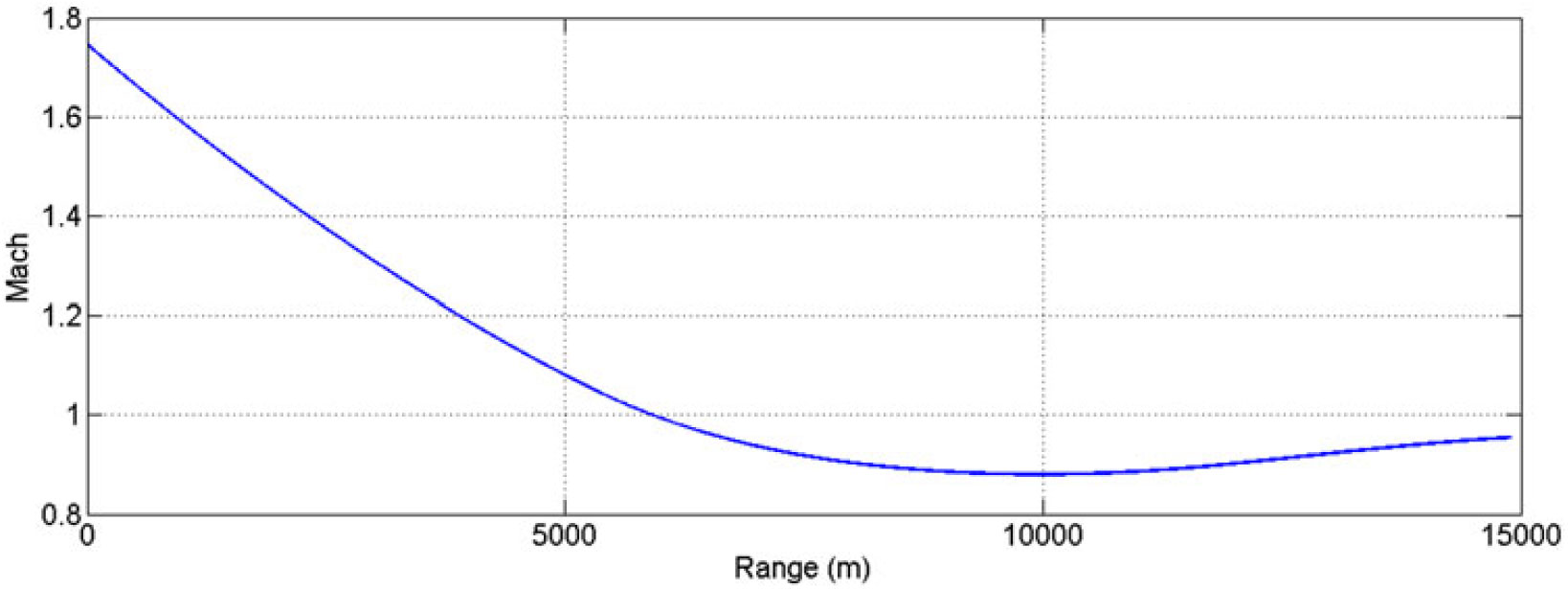
Figure 31. Mach vs range, charge 7 (MV 595 m/sec) at 600 mils.

At Charge 7, the amplitude of oscillations of resultant aerodynamic angle and equilibrium yaw is much higher as compared to low-speed flight at Charge 4. This effect is due to incorporation of Magnus effect in trajectory model that generated side force/moment, thereby, affecting the trajectory with respect to varying AoA and Mach speed. Since the force is a function of speed as well, at Charge 4, the oscillation effect is minimum. As the projectile suffers from continuously acting yaw of repose or equilibrium yaw, generated due to interaction of high gyroscopic effects and gravitational force, the Magnus forces and moments will be produced not only with changing AoA (α), but also due to sideslip angle AoS (β). Hence, the precession and nutation oscillation effects are magnified as depicted graphically in resultant aerodynamics angle and equilibrium yaw plots (Figs. 29 and 30).

Furthermore, Mach versus range plot at Charge 7 reveals that once the projectile reached apogee, the speed was reduced to the transonic region and the effect of the Magnus force varies as shown in the Cn_ρ and Cy_ρ plots, respectively. As a result, the oscillation increases at apogee, as is evident from the resultant aerodynamics angle and equilibrium yaw plots. The change in Magnus force as speed increases to transonic may be attributed to fluctuating wake effect and generation of corresponding vortices and their interaction with leading-edge separation bubbles, the trailing-edge vortices and spin-induced swirling flow in the wake region. The generation of a shock wave at transonic speed changes the flow dynamics with velocity and pressure variation behind the shock generation, and subsequently shows sudden variation in calculated dynamic coefficient. However, the pressure differential remains positive and doesn’t change the behavior with respect to speed/AoA as depicted in Figs. 16–18.

5.2 Internal dynamics and stability analysis

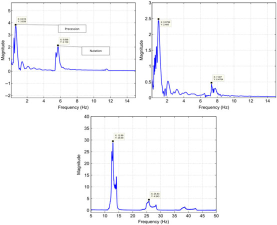
From classical aeroballistics theory, a spinning projectile executes two types of motions: precession and nutation^{(Reference Chughtai, Masud and Akhtar18)}. Precession is the low-frequency oscillation of the angular velocity vector about intended CG trajectory, whereas nutation is the high-frequency circular movement of the body axis around the velocity vector. The frequencies of the two motions corresponds to the two dominant resonance frequencies on the frequency spectral plot of aerodynamic angular motion of projectile in body-axis frame. The FFT analysis of resultant aerodynamic angle with respect to time for Mach speeds 0.7, 1.05 and 1.7 (Fig. 29) revealed specific trends in precession and nutation frequencies. The low-frequency first peak corresponds to precession frequencies, whereas the high-frequency second peak shows nutation frequencies (Fig. 32). As the Mach increases, so do the nutation and precession frequencies for each case. However, as compared to Charge 1 and 4, the precession and nutation frequencies for Charge 7 increase manifolds. This effect is because in descend phase after apogee, the Mach drops to transonic speed, as shown in Fig. 31, at which Magnus force and moment coefficient plots show gradient shift in results.

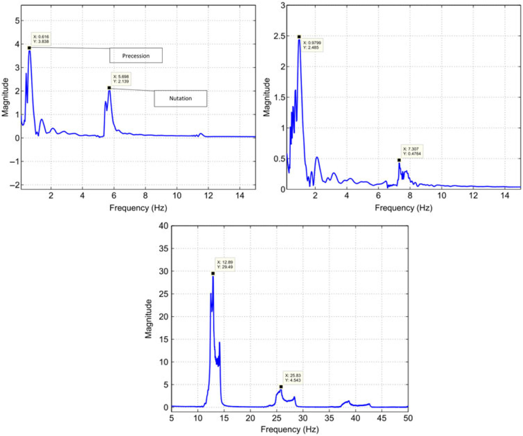
Figure 32. FFT plot charge 1 (MV 249 m/sec) (Left) – charge 4 (MV 350 m/sec) (right) – charge 7 (MV 595 m/sec) (below) at 600 mils.