


1.0 INTRODUCTION
The Copernicus Earth observation programme, previously called Global Monitoring for Environment and Security (GMES), is one of the two European flagship space programmes(Reference Reillon1). Copernicus gathers data for environmental and security applications and provides them on a free basis for the benefit of the civil community(2). The backbone of the programme’s space component is a fleet of spacecraft, the Copernicus Sentinels, manufactured in six series or platform families. Within each family, the spacecraft platform and mission objectives are adapted to gather specific observations(Reference Berger, Moreno, Johannessen, Levelt and Hansen3): radar altimetry for the Sentinel-1 family, multi-spectral imagery for the Sentinel-2 family, etc. In order to ensure continuous provision of data and optimal revisit time, a constellation of two spacecraft is in general operated per family. Since the first Sentinel launch in 2014, the size of the fleet has grown steadily and consists today of seven spacecraft: Sentinel-1A/B, 2A/B, 3A/B and 5P. The next launch is scheduled for 2021.
The purpose of this paper is the estimation of a realistic uncertainty on the state vector adjusted on-ground for the Sentinel spacecraft controlled at the European Space Operations Centre (ESOC) in Darmstadt, Germany. The state vector is adjusted to GPS positions provided in the spacecraft telemetry as part of the daily orbit determination process. The latter is a key component in the automatic set of routine operations performed by the Flight Dynamics team at ESOC. In particular, the uncertainty on the state vector is used as input parameter for covariance propagation and the estimation of collision probabilities with space debris(Reference Poore, Aristoff and Horwood4). An overly conservative estimate results in frequent collision warnings triggering the preparation of collision avoidance manoeuvers. The danger from an underestimated uncertainty is obvious. The recent collision event on Sentinel-1A, though in principle unavoidable because of the small size of the debris, is a reminder that the danger posed by space debris is real(Reference Kuchynka, Martin Serrano, Catania, Marc, Kuijper, Braun and Krag5).
This paper focuses on the Sentinel-1 (S1) and Sentinel-2 (S2) families. Sentinel-5P is a precursor for the Sentinel-5 family. Though also operated form ESOC, it is not considered in detail in this study. The Sentinel-3 family is operated by the European Organisation for the Exploitation of Meteorological Satellites (EUMETSAT). In the following sections, the individual spacecraft will be referred as S1A, S1B, S2A, and S2B. They fly at altitudes of about 700km on Sun-synchronous orbits with a frozen eccentricity and a closed repeat cycle. A phase difference of 180deg separates the A and B models. Orbit control is achieved by following reference ground-tracks within a control band of  $\pm$ 120m for S1 and
  $\pm$ 2km for S2. Orbit maintenance manoeuvers are executed weekly for S1 and approximately monthly for S2. Although the estimation of manoeuver performance is carried out in parallel with the OD process, the study of its effect on the state vector uncertainty is not considered in this paper.
The next two subsections describe the on-ground orbit determination (OD) process and the on-board GPS receivers. Section 2 briefly summarises the least-squares approach to OD. Section 3 presents the comparison of the estimated state vector with the orbit reconstructed from Precise Orbit Determination (POD). Section 4 compares the POD solutions directly with the GPS data and presents an analysis of the error present in the data. Finally, Section 5 describes a pragmatic approach for the problem of data whitening required for realistic covariance estimation.
1.1 Orbit determination process
Flight dynamics routine operations rely on a daily OD process. The determined state vector is propagated to provide the spacecraft reconstructed orbit, which in turn is used to generate flight dynamics products: station predictions, mission planning products, inputs to the space debris screening service, etc. The software running the OD relies on a complete dynamical model summarised, for S1 and S2, in Table 1. The determination arc spans over three days and ends a few hours before the time of the OD execution. Figure 1 illustrates the setup. GPS data is usually available without interruptions until the second half of the last day in the determination arc. The spacecraft state vector is estimated within the span of that arc together with two drag coefficients spanning each one day. The estimation of the drag coefficients is included to account for errors and uncertainties in the Earth atmosphere model. The middle one-day segment of the obtained orbit is merged with the reconstructed orbit from the previous day in order to become the new reconstructed orbit. In Fig. 1, this segment is indicated as the ‘archived arc.’ Note that the first day in the determination arc does not have an adjusted drag coefficient. We use instead the coefficient estimated for that segment in the OD carried out the day before. The OD process on any given day is thus partially constrained by the solutions obtained on the previous days.
Table 1 Dynamical model used in the OD process

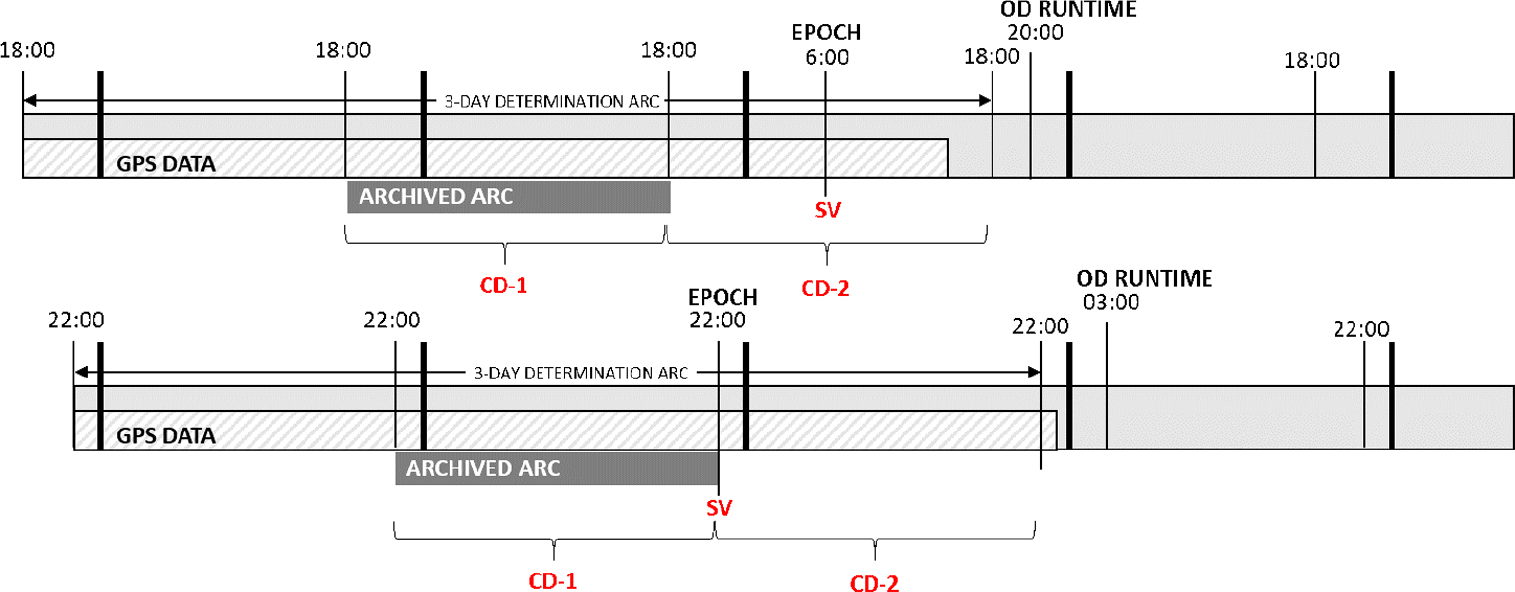
Figure 1. OD process setup for S1 (top) and S2 (bottom). In red, the estimated parameters: state vector (SV) at epoch and 2 daily drag coefficients.
1.2 Sentinel GPS receivers
The S1 and S2 spacecraft use the same GPS receiver manufactured by RUAG Space. The receiver tracks C/A and P(Y) codes on both L1 and L2 frequency bands. The receiver has two main functions: first computing in real-time the spacecraft position, the so-called navigation solution; and second, providing the carrier and code phase necessary for POD processing. The navigation solution relies on code phase pseudo-range measurements acquired simultaneously from up to eight GPS satellites. The use of both L1 and L2 frequency bands allows an autonomous correction of ionospheric delays.
Though S1 and S2 use the same receiver, the setup is different. In particular, the navigation solution computed on-board S1 is a least-squares fit of the spacecraft position to pseudo-range measurements. The solution is thus based on data available at a given instant in time. S2 uses a Kalman filter where a full dynamical model is sequentially adjusted to current and past pseudo-range measurements. Besides the state vector, the adjusted parameters include radiation pressure and drag coefficients as well as 3D empirical accelerations. The on-board dynamical model has the same level of fidelity as the model used in the on-ground OD process. The navigation solution is computed on-board at 1Hz, however the rate at which the solution is recorded in the telemetry is a user-defined parameter. For S1 the rate is set to 1/8Hz and further reduced in the OD, by downsampling, to 1/80Hz. For S2 the received rate is 1Hz, reduced in the OD to 1/10Hz.
The navigation solution provided in telemetry represents positions of the spacecraft centre of mass in the Earth-fixed frame. However, the solution computed on-board is obtained by adjusting the position of the receiver antenna to the pseudo-range measurements. In order to translate the antenna position to the centre of mass, the on-board software relies, in both the least-squares method and the Kalman filter, on the centre of mass to antenna vector in the spacecraft frame and the attitude of that frame with respect to the orbital frame. These parameters are considered as constant, though they may be updated by telecommand. In practise, the values vary slightly with time. The centre of mass varies with fuel consumption and nominal attitude follows yaw steering laws. S1 has a fixed solar array and executes manoeuvers in its nominal attitude. In contrast, the centre of mass of S2 varies with the rotation of the solar array and slews are required to execute manoeuvers.
The RUAG receiver is also flown on Sentinel-3. A different type, manufactured by Airbus, is flown on Sentinel-5P. The receiver operates with L1 C/A code only. Though capable of providing pseudo-range measurements, the data are currently not transmitted in telemetry. In consequence, POD is not available for Sentinel-5P.
2.0 LEAST-SQUARES ESTIMATOR
The on-ground OD relies on a least-squares fit of the state vector and of the atmospheric drag coefficients to the navigation solution data available in the three-day determination arc. In order to account for non-linearity, the fit is iterated. The linear model is described by
 \begin{eqnarray*}z = M \beta + \epsilon, \end{eqnarray*}
where z represents the measurements, M the partials matrix,  $\beta$ the estimated parameters and
  $\epsilon$ the measurement error. The error is assumed to have an expectation of zero and a constant covariance
  $C_\epsilon$. The least-squares estimation of
  $\beta$ is
 \begin{eqnarray*}\tilde{\beta} = (M^T M)^{-1} M^T z. \end{eqnarray*}
Figure 2. Comparison of the S1A (top) and S2A (bottom) reconstructed orbits with POD in the orbital frame. The dots on the x axis indicate simple (white) and multiple (red) manoeuvers.
The propagation of linear dependencies through expectation and covariance guarantees that the estimator is unbiased, that is  $E(\tilde{\beta})=\beta$. Its covariance is
 \begin{eqnarray*}\mbox{Cov}(\tilde{\beta}) = (M^T M)^{-1} M^T C_\epsilon M (M^T M)^{-1}. \end{eqnarray*}
 The uncertainty of the estimated parameters naturally depends on  $C_\epsilon$. Once this is known, it is usually translated into a weight matrix W such as
  $C_\epsilon = W^T W$. This allows rewriting the linear model in terms of the weighted observations
  $z' = W z$ and weighted partials
  $M' = W M$. The covariance of the estimates then simplifies to
 \begin{eqnarray*}\mbox{Cov}(\tilde{\beta}) = (M'^T M')^{-1}. \end{eqnarray*}
3.0 COMPARISON OF THE RECONSTRUCTED ORBIT WITH POD
POD orbits are regularly computed for both S1 and S2. The computations are carried out for the Sentinel Payload Data Ground Segment by the Copernicus POD service(Reference Fernandez, Escobar, Heike and Femenias6). They are also carried out by different organisations, including the ESOC Navigation Support Office, for validation and quality control purposes. The accuracy of the POD positions is on the order of a few cm. For the purpose of this study, they are considered as a substitute for the real spacecraft trajectory. Figure 2 compares in the orbital frame the S1A and S2A reconstructed orbits with POD orbits provided by the ESOC Navigation Support Office. The same comparisons for S1B and S2B are not shown as they are similar to those of S1A and S2A. Recall that the reconstructed orbit is made of one-day arcs merged together. The accuracy of each of these arcs is the same as the accuracy of the state vector estimated in the OD. The differences in Fig. 2 are thus representative of the accuracy of the estimated state vector.
For both S1 and S2, the 1-sigma errors are 0.4, 0.2 and 0.1m in the along-track, cross-track and radial directions respectively. Errors in velocities in the three directions are 0.1, 0.2 and 0.4mm/s. The evolutions of the velocity errors in along-track, cross-track and radial mirror to a large extent the position errors in radial, cross-track and along-track. The velocity error is computed by projecting the difference in inertial velocities onto the orbital frame. In consequence, the mirroring is not due to a kinematic effect introduced by the rotation of the orbital frame. It is due to correlations between the along-track, cross-track and radial components of the position and velocity at epoch estimated in the OD.
The spikes observed in Fig. 2 correspond in general to manoeuvers, in particular multiple manoeuvers executed in sequence such as collision avoidance manoeuvers or out-of-plane manoeuvers followed by in-plane corrections. More rarely, the spikes are due to an operational event, such as the failure of the automatic OD process over a weekend. After several days of failed archiving, the reconstructed orbit contains propagation arcs which rapidly degrade in accuracy.
A bias in the along-track direction of about  $-0.5$m is apparent for S2A. A smaller bias,
  $-0.2$m, is also present on S2B. The Kalman filter thus estimates for S2A and S2B the trajectory of a point slightly behind the real centre of mass. The effect could be due to imperfect values on-board for the centre of mass to antenna vector. It could also come from imperfect timing of the GPS data in the telemetry.
4.0 COMPARISON OF THE GPS NAVIGATION SOLUTION WITH POD
Comparing POD orbits with the navigation solution extracted from telemetry instead of the reconstructed orbit makes possible the direct analysis of the measurement error involved in the OD process.
4.1 Comparison in the spacecraft body frame
The differences between the navigation solutions and the POD, expressed in the spacecraft body frames, are represented in Fig. 3. The evolutions for S1B and S2B are not shown, but are similar. Figure 3 can also be interpreted as the representation of the navigation solution error in the orbital frame, since the S1 and S2 attitudes are approximately constant in the orbital frame. The body x axes are aligned with the flight direction. The z axes point roughly towards the Earth. In addition to the measurement error, the figure shows a running average over a 10 min interval. For the Kalman filter solution on S2A, the running average is almost undistinguishable from the error itself.

Figure 3. Errors over a one-day interval in the navigation solution for S1A (top) and S2A (bottom) in spacecraft body frame. A running average is shown in black and a global average in red.
We observe a  $-0.5$m bias on the x component of S2A corresponding to the along-track bias observed earlier in Fig. 2. Smaller, but non-negligible biases appear on the other components. For S1A, only the z component is significantly biased with a value of 0.5m. Though Fig. 3 represents one day of data, the values of the biases remain constant from day to day, at least over a period of a few months. The biases could be removed by adjusting the on-board values of the centre of mass to antenna vector. Note that any bias in the spacecraft body frame other than along the x axis will not represent a realistic orbit and will be mostly ignored by the OD process. On S2, any imperfection in the antenna vector creates an error in the Kalman filter dynamical model, equivalent to an error in the filter input data. Similarly to the on-ground OD process, the error will largely be eliminated by the on-board fit, however it will be reinjected in the final navigation solution when translating the adjusted antenna position back to the spacecraft centre of mass.
4.2 Heteroscedasticity
The representation of the S1 navigation solution error in the Earth-fixed frame reveals a time-dependent structure in the variance of the data. The evolution of the error in the Earth-fixed frame is represented on Fig. 4. The figure shows also a running average over a 10 min interval. The estimate of the variance is obtained by subtracting this average from the signal and computing the sample variance over the same interval of 10 min. The resulting estimate of the variance is shown on Fig. 5. The changes in variance on any given coordinate correlate approximately with the evolution of the same coordinate of the spacecraft position. The variance on x is maximum when the position x coordinate is also at its maximum, that is when the spacecraft crosses the equator near 0 longitude. Conversely, it is at its minimum when the position x coordinate is at its minimum. The effect is explained by the concept of geometric dilution of precision (GDOP)(Reference Langley7). At any instant, the visible GPS satellites are positioned to best constrain the spacecraft position in one particular direction. For example, at the equator near zero longitude, the y coordinate is well constrained as satellites are available above and below the equator. On the other hand, the Earth hides half of the GPS satellites that would best constrain the x coordinate. This effect, together with spacecraft polar orbit and Earth rotation, gives rise to the pulsations observed in Fig. 5. Though heteroscedastic, the variance of the S1 data is less than 2m in the x and y coordinates and less than 3m in the z coordinate. For S2, given the small magnitude of the signal remaining after removing a running average, the variance of the data was not analysed.

Figure 4. Idem as Fig. 3, except in the Earth-fixed frame.

Figure 5. Standard deviation in the S1A GPS navigation error, computed in the Earth-fixed frame and estimated over intervals of 10 min. In grey, scaled evolution of the spacecraft x, y and z coordinates in the Earth-fixed frame.
The spacecraft receiver provides together with the navigation solution a so-called quality index. The index combines the current GDOP with the residuals obtained on the pseudo-range measurements to an average 3D uncertainty on position. The quality index represents well the evolution of a combined variance derived from the evolutions in Fig. 5. However, it cannot be immediately translated into variances on the individual coordinates to be used in a refined weighting scheme.
4.3 Non-stationarity
The estimation of realistic uncertainties in the OD process depends on a realistic covariance for the measurement error. Given that comparisons with POD make possible the computation of the actual errors in the navigation solutions, the error covariance could a priori be estimated numerically. The estimation consists in computing a sample variance over a sufficiently long interval, say one day. This provides the value for the diagonal elements of the covariance matrix. The non-diagonal elements are derived from sample covariances of the data with itself, but lagged by one step, two steps, etc. The approach assumes that the estimated covariance is stationary or, in other words, that the estimation run over one particular interval is representative of the covariance on any other interval.
In the following discussion, we assume that the error has zero expectancy over one day and its variance is roughly constant. This is confirmed by the absence of significant bias in Fig. 4 and the moderate heteroscedasticity observed in Fig. 5. The structure of a sample covariance matrix is conveniently represented by the autocorrelation function, which represents the evolution of covariance as a function of lag. The covariances are normalised by the sample variance so the value at lag zero is always one (the covariances become correlation coefficients). Figure 6 shows the autocorrelation function for the x component of S1A data computed over two different days. A similar plot has been computed for S2A. The data for S2A have been re-sampled to 1/80Hz in order to obtain a plot comparable with the S1A plots. The covariance matrices represented in the plots are not trivial. Statistically significant elements appear for more than 70 lines off the diagonal. The evolutions in Fig. 6, in particular the values of the autocorrelation coefficients persisting into high lags, are typical of non-stationary time series. The non-stationarity is also apparent in the different shapes of the autocorrelation function obtained for S1A for two different days. The non-stationary nature can be due either to a deterministic process, in other words a function of time, or to a non-stationary stochastic process. From Section 4.1, we know that it is at least partially due to a deterministic process equivalent to a constant bias in the spacecraft body frame.

Figure 6. Autocorrelation function computed over one day of data on the x component of the navigation solution error for S1A and S2A. The horizontal lines indicate a 95% significance interval with respect to white noise.
Stationarisation of the error data is necessary for the estimation of a constant error covariance matrix. One approach to stationarisation is differentiation. Replacing the S1 position measurements at 1/80Hz with position differences at 1/40Hz resampled back to 1/80Hz leads to approximately the same size of data. The autocorrelation function then contains no spikes above the significance level for lags beyond 0. The error appears as almost perfectly white. A similar result can also be achieved by further downsampling the data from 1/80 to 1/800Hz. We are then left with about 10 points per orbit. Weighting the differenced data according to its variance and re-running the OD process shows that the covariance of the estimated parameters becomes realistic. On the other hand, the quality of the OD is degraded. Instead of estimating the state vector to better than 0.5m, it is estimated with an uncertainty of a few meters or worse. The result can be somewhat optimised by taking differences of points further apart, but this eventually starts re-introducing spikes in the autocorrelation function. The two described approaches to stationarisation and whitening do not rely on any identified characteristic of the error signal. They operate by merely decreasing the signal-to-noise ratio in the errors to the level where the signal becomes masked by the noise. Naturally, a decrease in the signal-to-noise ratio in the errors is accompanied by a decrease in the signal-to-noise ratio in the overall data. The same whitening effect is achieved by simply adding white noise to the data until the non-stationary signal in the errors becomes negligible. Contrary to differencing, this has the advantage of not degrading the quality of the estimation as the whitening is achieved by merely applying underestimated weights in the least squares.
The exact weighting scheme to apply in order to obtain a realistic covariance needs to be derived from past error evolutions such as those represented in Fig. 4. The magnitude of noise necessary to mask the signal depends not only on the signal magnitude, but also on its shape. More precisely, it depends on the magnitude of the errors projected on the vector space spanned by the partials of the estimated parameters. An error that is orthogonal to the partials will not affect the estimates and does not need to be masked. On the other hand, an error that represents a realistic orbit, and thus is well represented by a combination of the partials, will require a large amount of masking. This will be the case for the 0.5m along-track bias on S2A. In the following section, the weights are estimated by re-running the OD process for S1A and S2A on two months of data and inflating the covariances to the point where they become realistic.
5.0 OD PROCESS WITH REALISTIC COVARIANCES
The setup for the OD process used to generate the S1 and S2 reconstructed orbits is difficult to reproduce exactly. As described in Section 1.1, the process keeps some memory of the OD from the previous days. More importantly the exact outcome of the OD depends on the time interval covered by the GPS data available on the Flight Dynamics system at the time of the run, which might vary from day to day. The data is automatically extracted from telemetry files at fixed time intervals, however the availability of the telemetry files is affected by transfer and processing delays.
The determination of a proper weighting scheme for S1 and S2 is based on a simplified OD setup. GPS data used in the simplified process spans all three days of the determination arc and we estimate a drag coefficient for each day. A further simplification is that manoeuver performance is not estimated, instead the accelerations calibrated in the routine OD process are used as fixed parameters. The sampling of the GPS data used in the OD is identical to the one used in routine operations: 1/80 and 1/10Hz for S1 and S2 respectively. Figure 7 shows the difference between the state vector estimated in the simplified OD and the POD orbits for S1A. The vertical bars represent a 1-sigma uncertainty derived from the least-squares covariance. In order to obtain a good match between the estimated uncertainties and the observed differences with the real state vector (POD solution), the weight of the GPS data had to be set at 10m. This amounts to about 5 times the magnitude of the average signal in Fig. 4. The error in the determined state vector is consistently well predicted by the covariance uncertainty. The frequent manoeuvers appear to have little to no effect.

Figure 7. Comparison between POD and the S1A state vector with measurement weights at 10m.
For S2A, in order to obtain realistic uncertainties, the data needs to be weighted by 60m. The differences with POD and the corresponding uncertainties are shown on Fig. 8. In four cases, the 1-sigma uncertainty bars and the observed difference with POD appear inconsistent. In particular, this happens for the 15/09. The divergence for this day was also observed in the operational orbit and appears in Fig. 2 as a spike in the along-track direction. The inconsistencies for the other three days are due to a double manoeuver executed on the 20/09. The manoeuver is an out-of-plane change accompanied by an in-plane correction and it is the only manoeuver executed during the two-month period shown in Fig. 8. The manoeuver size is more than an order of magnitude larger than the largest manoeuver executed on S1A.

Figure 8. Comparison between POD and the S2A state vector with measurement weights at 60m. Four particular days are marked in red: 15/09 and a three-day arc around 20/09.
The larger weight value necessary for S2A is partially expected. S2 uses 8 times more data points than S1. In order to mask the same error for N times more points, the weight value should be increased by a factor of  $\sqrt{N}$, in this case a factor of
  $\sqrt{8} \sim 3$. In practice the weight value had to be increased by a factor of 6. As discussed earlier, the magnitude of the white noise that has to be applied to the data in order to obtain a realistic covariance depends not on the error magnitude but rather on the magnitude of its projection on the space spanned by the partials.
Due to the along-track bias, the magnitude of projected error is significantly larger for S2A than for S1A. The differences in S2A positions and the corresponding uncertainties obtained by scaling the S1A weights by a factor of 3 instead of 6 are shown on the top part of Fig. 9. Note that the 1-sigma uncertainty bars are not representative of the variance in the observed difference with POD. The bottom part of the figure shows the same plot obtained after correcting the estimated positions for a 0.5m along-track bias. The errors and estimated uncertainties are now consistent. The weights of 60m, instead of the expected 30m, are needed mostly to absorb the along-track bias.

Figure 9. Idem as Fig. 8, except only positions are shown and the weights are 30m. The bottom plot has been corrected for a shift of 0.5m in the along-track direction.
6.0 DISCUSSION
Our objective was the estimation of realistic uncertainties on the S1 and S2 state vectors. We carried out an error analysis of the navigation solution data made possible by comparison with POD. The error is heteroscedastic, with variance pulsating between 0.5 and 3m because of periodic changes in GDOP. More importantly, the error is non-stationary partially due to deterministic trends. These un-modelled time dependent effects detected in the input data could in principle be characterised for each spacecraft and removed. The detailed analysis of the effects followed by the implementation of their mathematical model in the OD is however beyond the scope of operational activities. It is also beyond the intended use of the on-board navigation solution.
In order to derive realistic uncertainties for space debris screening, the proposed approach is to use underestimated weights on the data to decrease the signal-to-noise ratio in the error to a level where uncertainties become dominated by white noise. In practise, we have used two-months arcs of past data to calibrate weights against POD and reflect in the least-squares covariance the realistic uncertainties of the OD process. The approach is generic in the sense that it can be directly applied to any spacecraft with available POD. However, the weights are spacecraft specific as they depend on the magnitude and shape of the error in data.
Furthermore, the errors depend on the sampling rate of the data. The dependency is in  $\sqrt{N}$ where N is the number of data points. If for some reason the GPS data becomes significantly sparse, for example because of problems preventing the processing of telemetry files on-ground, the estimated uncertainty on the state vector will become overestimated. Since the data weights are calibrated on past data, they will be correct only to the extent that the calibration interval is representative of the future. It is thus recommended to repeat the calibrations at regular intervals or simply to routinely compare the state vector derived in the OD with POD solutions.
For spacecraft without available POD, such as Sentinel-5P, an alternative approach could rely on comparisons of state vectors derived from different determination arcs spanning for example three days before and three days after the epoch of the estimated state vector. Using this cross-validation approach to estimate the data weights has the disadvantage that any part of the error in the data representing a meaningful orbit will be ignored. In particular, the along-track bias observed for S2 would not be detected.
In all previous discussions we considered the error in the data as the only source of errors in the estimated parameters. The inflated covariances based on the POD comparison will absorb this error but also any other such as omitted variables and imperfections in the dynamical model. For example, the average error in the S1A state vector decreased significantly in 2017 after a change in the solar radiation pressure coefficient in the OD dynamical model. The change was triggered by observing a mismatch in the eccentricity evolution with respect to an analytic prediction(Reference Sanchez, Martin Serrano and Mackenzie8). The data before this change is represented in grey on Fig. 2. Running the calibration of the weights on a data arc before June 2017 would have reflected the imperfection in the dynamical model, inflating the covariance correspondingly.
Given that the state vector uncertainties are on average better than 0.5m in position and 0.5mm/s in velocity, the spacecraft predicted position for an interval of a few days will be on the order of metres in the cross-track and radial directions. This uncertainty is of about the same size as the spacecraft itself. The uncertainty in the along-track direction is driven by the uncertainty in semi-major axis. The latter is about 0.05m for both S1 and S2. The error in semi-major axis induces a linear drift of 8m per day. The typical day-to-day variation in the drag coefficient is about 0.5, equivalent to a quadratic drift in the along-track direction of 3m in one day. In three days, the drag uncertainty will amount to more than 27m, while the semi-major axis contribution will be about 24m. For close approach events three days or less in the future, and contrary to the cross-track and radial directions, the collision probability will be affected by the along-track uncertainty in the predicted spacecraft position. For approaches further in the future, this uncertainty becomes dominated by uncertainties in drag.
Our study ignored the effects of manoeuvers on the estimated state vector uncertainty. The effects may be negligible on S1 because of relatively small manoeuvers. They are not negligible for S2 as shown on Fig. 8. In consequence, the manoeuver components need to be taken into account in the estimation of the state vector covariance, at least as consider parameters.
7.0 CONCLUSION
The uncertainties in the S1 and S2 operational orbits are similar and amount to 1-sigma errors of less than 0.5m and 0.5mm/s. In addition, S2 positions are affected by a constant along-track bias. Non-stationary errors in the navigation solution make impossible their characterisation with a constant covariance. Unless the non-stationary part is modelled, the whitening of the errors can be achieved by decreasing the signal-to-noise ratio in the data and the errors by applying constant but underestimated weights. We have shown on historical S1A and S2A data that the approach indeed allows the computation of realistic covariances on the state vector estimated in the OD process.
ACKNOWLEDGEMENTS
The Navigation Support Office at ESOC has kindly provided access to the Sentinel POD orbits. The first author thanks GMV INSYEN for the organisational and financial support necessary for preparing the paper.


