2.0 ESTABLISHING AN INITIAL SET OF OPTIMAL CONTROL LAWS

In this sub-section, the formulation for the prediction of the linearised, quasi-steady subsonic aerodynamic loads is briefly revisited to explain how a preliminary linear state-space model and a set of optimal control laws can be established. Generally, if one uses the DLM, given a reference length such as the root chord ${c_r}$ , the free stream density ${\rho _\infty }$ and the free stream flow velocity ${U_\infty }$ , one can construct the generalised aerodynamic forces matrix defined by

(1) \[Q\left( k \right) = \frac{1}{2}{\rho _\infty }U_\infty ^2c_r^3\int_{{S^*}} {\left( {{z_i}\left( {{x^*},{y^*}} \right)/{c_r}} \right)} \Delta {C_{p,j}}\left( {\left( {{z_j}{\text{ }}/{c_r}} \right),{x^*},{y^*},k,{M_\infty }} \right)d{S^*},\]

where ${z_j}$ is the vibration mode shape of the structure in the ${j^{th}}$ mode, ${S^ * }$ is the non-dimensional planform area, ${x^ * }$ and ${y^ * }$ are the non-dimensional coordinates of a point in the planform, $k$ is the reduced frequency and ${M_\infty }$ is the free stream Mach number, the ratio of the free stream flow velocity to the local speed of sound. In the above equation for the generalised aerodynamic force matrix, the integration is performed over the planform surface area. The modal displacements and slopes at the sending and receiving points in the DLM code are obtained by spline interpolation of the modal displacements at nodes of the structural model. The matrix ${\bf{Q}}\left( k \right)$ is generally complex. If one assumes a matrix Padé approximant representation, the matrix ${\bf{Q}}\left( k \right)$ may approximated as

(2) \begin{equation}{\bf{Q}}\left( k \right) \cong {{\bf{Q}}_0} + ik{{\bf{Q}}_1} + {\left[ {{\bf{I}} + ik{{\bf{Q}}_p}} \right]^{ - 1}}{{\bf{Q}}_r},\end{equation}

where ${{\bf{Q}}_0}$ and $ik{{\bf{Q}}_1}$ are the steady-state and low-frequency asymptote, which can be computed independently from the steady-state and low-frequency asymptotes of the subsonic kernel function as outlined by Vepa^{(Reference Vepa5)}. If one assumes that the augmented poles are relatively fast, which is usually the case, then it is possible to set ${{\bf{Q}}_p} \approx {\bf{0}}$ . Consequently,

(3) \begin{equation}{\bf{Q}}\left( k \right) \approx {{\bf{Q}}_0} + ik{{\bf{Q}}_1} + {{\bf{Q}}_r}.\end{equation}

Generally, the matrices ${{\bf{Q}}_r}$ (the residue matrix) and ${{\bf{Q}}_p}$ (the matrix related to the poles corresponding to the augmented states) are constructed by matching the matrix ${\bf{Q}}\left( k \right)$ to the coefficient matrices in the matrix Padé approximant representation at some low value of the reduced frequency $k = {k_f}$ close to the estimated flutter reduced frequency. Then, assuming that $k$ is small, it follows that

(4) \begin{equation}{{\bf{Q}}_0} + {{\bf{Q}}_r} \cong {\left. {{\mathop{\rm Re}\nolimits} \left( {{\bf{Q}}\left( k \right)} \right)} \right|_{k = {k_f}}} = {\mathop{\rm Re}\nolimits} \left( {{\bf{Q}}\left( {{k_f}} \right)} \right).\end{equation}

Thus ${\bf{Q}}\left( k \right)$ , computed by the DLM, may be approximated by the quasi-steady approximation, which corresponds to the zeroth-order matrix Padé approximant and is given by

(5) \begin{equation}{\bf{Q}}\left( k \right) \cong {\mathop{\rm Re}\nolimits} \left( {{\bf{Q}}\left( {{k_f}} \right)} \right) + ik{{\bf{Q}}_1}.\end{equation}

The approximation involves no augmented states and can be used to construct a linear state-space model of the aeroelastic system. Thus, given the mass matrix ${\bf{M}}$ , the stiffness matrix ${\bf{K}}$ , of the structural system, assuming a suitable model for the structural damping factor $g$ , so the structural damping matrix is ${\bf{C}} = g{\bf{K}}$ , and that any control surface that may be present is locked in its equilibrium position, the equations of motion of the wing in terms of the vector of generalised modal displacement amplitudes ${\bf{q}} = {\left[ {{q_j}} \right]^T}$ are

(6) \[M\ddot q + C\dot q + Kq = Re\left( {Q\left( {{k_f}} \right)} \right)q + \left( {{c_r}/{U_\infty }} \right){Q_1}\dot q.\]

When the modal displacements are normalised by the square root of the generalised masses, the mass matrix is given by ${\bf{M}} = {\bf{I}}$ and the coordinates ${\bf{q}}$ are the principal coordinates. In the presence of a control surface such as a trailing-edge partial-span flap, assuming that the flap is actuated relatively slowly, the equations of motion defined by equations (6) are now extended to include the quasi-steady generalised aerodynamic forces due to the flap angular displacement $\eta $ and expressed as

(7) \[M\ddot q + C\dot q + Kq = Re\left( {Q\left( {{k_f}} \right)} \right)q + \left( {{c_r}/{U_\infty }{\text{ }} - {U_\infty }} \right){Q_1}\dot q + Re\left( {{Q_\eta }\left( {{k_f}} \right)} \right)\eta .\]

The equations of motion defined by equations (7) may then be cast in state-space form, where the state vector is the combination of both ${\bf{q}}$ and ${\dot{\bf{q}}}$ , and written as

(8) \begin{equation}{\dot{\bf{x}}} = {\bf{Ax}} + {\bf{B}}\eta.\end{equation}

Now it is completely feasible to construct an optimal control law based on the above model formulation, defined by equation (8). The optimal control is assumed to minimise a cost function of the form

(9) \begin{equation}J\left( {{\bf{x}}\left( {{t_0}} \right),{t_0}} \right) = \int_{{t_0}}^{{t_f}} {\left( {{{\bf{x}}^T}{{\bf{Q}}_x}{\bf{x}} + {{\bf{u}}^T}r{\bf{Ru}}} \right)dt} + {{\bf{x}}^T}\left( {{t_f}} \right){{\bf{Q}}_f}{\bf{x}}\left( {{t_f}} \right),\end{equation}

where $r$ is a scalar used to alter the control weighting matrix ${\bf{R}}$ in the formulation of the optimal control law synthesis, ${{\bf{Q}}_x}$ is the state vector weighting matrix, and ${{\bf{Q}}_f}$ is the weighting matrix for the state vector at the final time $t = {t_f}$ . For the single input case, ${\bf{R}} = 1$ . The steady-state control law takes the form

(10) \[\eta = u = - \left( {1/r} \right){R^{ - 1}}{B^T}{P_\infty }x \equiv - {K_f}x,\]

where ${{\bf{P}}_\infty }$ satisfies an algebraic Riccati equation. Thus, given a range of monotonically increasing free stream Mach numbers ${M_{\infty ,j}}$ , $j = 1,2, \cdots ,$ as well as a set of values for the relative weighting scaling parameter $r$ , one can construct families of control laws with differing closed-loop stability characteristics. Each of these control laws may then be used with the open-loop dynamics, reformulated in the transonic domain based on the TSD theory, to study the closed-loop behaviour of the aeroelastic system. The control laws, however, are no longer optimal and can at best be considered as near optimal. To match the control laws to the transonic dynamic model and the TSD theory, the control law calculations are carried out at a set of specific flight conditions.

The parameter r, in accordance with optimal control theory, is the ratio of the maximum magnitude of an element in the state vector to the maximum magnitude of the control input. It is a measure of the performance that is expected or delivered by the optimal control law. When r is large, the maximum magnitude of the control input relative to the magnitude of the state is very small. In this case, the magnitude of the largest element in the state vector is large; it asymptotically tends to the case when there is no or a small control input. On the other hand, when r is small, the control input is significant as a large control input must be used. The case of $r \approx 1$ represents the balanced case where the magnitude of the control used is of the same order of magnitude as the state vector. In this paper, it provides us with a single scalar parameter that we can vary to obtain a large distribution of control laws, which we could use to find a near-optimal solution, as our problem is essentially non-linear.

Alternative methods for synthesising the preliminary control law, such as transonic linear small perturbation theory, time-domain fitting of the unsteady loads, eigensystem realisation algorithm and the transonic linear full potential method, were also explored. However, the doublet lattice method coupled with the zeroth-order matrix Padé approximant provided the fastest method for synthesising the large number of preliminary control laws needed to make an informed choice of the final control law. By using a linear model such as the DLM, the search for a suitable control law is essentially carried out over a one- rather than multi-dimensional space.

3.0 CONTROL LAW VALIDATION IN THE TRANSONIC DOMAIN

In the transonic domain, based on the TSD formulation, the equations of motion of the vibrating wing, including the partial-span trailing-edge flap, take the form

(11) \begin{equation}{{\bf{M}}{\ddot{\bf{q}}}} + {\bf{C}}{\dot{\bf{q}}} + {\bf{Kq}} = {{\bf{Q}}_{tsd}}\left( {{\bf{q}},{\rm{ }}{\dot{\bf{q}}},{M_\infty }} \right) + {{\bf{Q}}_{tsd,\eta }}\left( {{\bf{q}},{\rm{ }}{\dot{\bf{q}}},{M_\infty }} \right)\eta,\end{equation}

where the vectors ${{\bf{Q}}_{tsd}}\left( {{\bf{q}},{\rm{ }}{\dot{\bf{q}}},{M_\infty }} \right)$ and ${{\bf{Q}}_{tsd,\eta }}\left( {{\bf{q}},{\rm{ }}{\dot{\bf{q}}},{M_\infty }} \right)$ are obtained numerically using a code based on the TSD formulation^{(Reference Kwon, Kim and Lee44)}. When the feedback control law developed in the preceding section is used, the corresponding closed-loop equations of motion take the form

(12) \begin{equation}{\bf{M}}{\ddot{\bf{q}}} + {\bf{C}}{\dot{\bf{q}}} + {\bf{Kq}} = {{\bf{Q}}_{tsd}}\left( {{\bf{q}},{\dot{\bf{q}}},{M_\infty }} \right) - {{\bf{Q}}_{tsd,\eta }}\left( {{\bf{q}},{\rm{ }}{\dot{\bf{q}}},{M_\infty }} \right){{\bf{K}}_f} \left[ \begin{array}{cc}{{{\bf{q}}^T}} & {{{{\dot{\bf{q}}}}^T}}\end{array} \right]^T. \end{equation}

It must be emphasised that, in the above equations (11) and (12), the aerodynamic load vectors are computed by the use of the TSD theory, while the control gain vector ${{\bf{K}}_f}$ , in equation (12), is obtained by using a linear model of the aeroelastic system based on the DLM. However, the DLM is also a linear potential flow-based method, although it is also a boundary element method based on the linearised kernel function formulation of the potential function.

To match the control laws to the transonic model, the response calculations were carried out at the same set of specific flight conditions as used earlier for the computation of the control laws. As the model used for the synthesis of the linear control laws and the model used for the closed-loop validation are different, the control laws can, at best, be only considered to be sub-optimal, although it is possible to show in principle, on the basis of the solution of the inverse optimal control problem, that there exists an optimising cost function associated with the closed-loop model. The numerical solution of the closed-loop equation (12) is obtained by a time-marching method. By proceeding monotonically from the open-loop stable case, for lower values of ${M_\infty }$ , to the open-loop unstable cases corresponding to higher values of ${M_\infty }$ , the responses are obtained quite quickly. The closed-loop characteristics are assessed, and from the responses, the decay rate and oscillation frequency are obtained. By suitable interpolation, when the decay rate is equal to zero, the flutter Mach number and the flutter frequency are then obtained, provided they lie within the envelope of the cases considered. In most cases, the closed-loop response was adequately stable and the corresponding flutter Mach number and flutter frequency are beyond the aircraft’s desired flight envelope.

4.0 APPLICATION TO BENCHMARKING EXAMPLES

The methodology was applied to two benchmarking examples, the first a low-aspect-ratio wing and the second a moderately high-aspect-ratio wing. The first is the AGARD 445.6 wing model, proposed by Yates^{(Reference Yates45)}, which is a standard aeroelastic configuration used for validation purposes. Experimentally obtained transonic flutter characteristics of a similar wing planform were reported earlier.

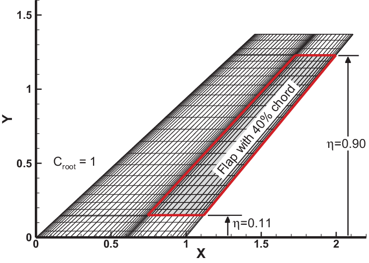
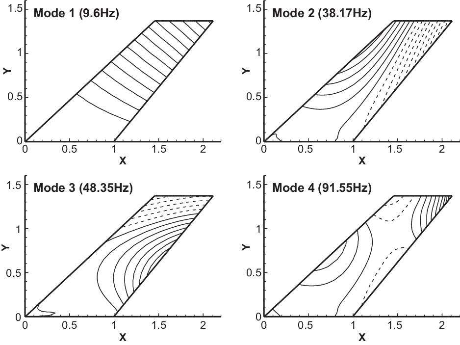
The AGARD 445.6 wing is a swept-back wing, with a quarter-chord sweep angle of 45° and a NACA 65A004 aerofoil cross-section, as shown in Fig. 1. It has a panel aspect ratio of 1.65 and a taper ratio of 0.66. In the DLM code, it is modelled as a flat plate. Continuous representations of the first four mode shapes of the AGARD 445.6 planform, obtained after splining the discrete mode shape data using the infinite plate surface (IPS) spline method proposed by Harder and Desmarais^{(Reference Harder and Desmarais46)}, which assumes a set of discrete data points lying within an infinite flat plate, are shown in Fig. 2.

Figure 1. The AGARD 445.6 planform with trailing-edge flap and the aerodynamic grid.

Figure 2. Illustration of the first four mode shapes of the AGARD 445.6 wing smoothed by the IPS method.

The nominal flight condition for this example is an altitude of 10,000m. The corresponding atmospheric density, temperature and the speed of sound were estimated from the properties of the international standard atmosphere. The structural damping factor was assumed to be $g = 0.03$ , as it is particularly important to damp the higher-frequency modes.

The second benchmarking model used for validation is the NASA Common Research Model (CRM), which consists of a contemporary supercritical transonic wing (and a fuselage). The CRM is designed for a cruise Mach number of ${M_\infty } = 0.85$ . The corresponding design coefficient of lift is ${C_L} = 0.5$ . The aspect ratio of the wing planform is equal to 9.0, and the quarter-chord sweep angle is 35°.

Initially, the structural modes of the wing models were computed using a matching structural grid and the finite element method and verified with published data, provided in the paper. The primary modification introduced was the inclusion of a servo-controlled flap, which was assumed to be deflected relatively slowly. The flap was used only to modify the unsteady aerodynamic loading on the wing. When any modifications were made to the wing, the structural modes were re-computed using a similar matching structural grid and the finite element method with the flap actuator fixed rigidly, so the flap remained without any rotation in its initial equilibrium position. The same method was used for all the benchmarking models that were considered. In the second example, the flap was assumed to be much smaller relative to the wing than in the first example, but it is more realistic. The non-dimensional CRM planform is illustrated in Fig. 3. The geometry and model files are available in the public domain^{(Reference Rivers47)}.

Figure 3. Non-dimensional CRM planform with a flap of 23% wing chord.

5.0 TYPICAL RESULTS AND DISCUSSION

The first example was the AGARD 445.6 three-dimensional wing. In this example, to capture the closed-loop flutter point, the response calculations were done at several sets of flight Mach number, corresponding to the range of values of the flutter speed index ${U_\mu }$ , and the cost function relative weighting scaling parameter $r$ , defined earlier in equations (9) and (10). Based on the quasi-steady DLM, the wing flutters in open loop, at ${M_\infty } = 0.86$ .

Based on the nonlinear TSD aerodynamics, the onset of flutter without any control inputs occurs at about ${M_\infty } = 0.56$ . Recall that the non-dimensional flutter speed index ${U_\mu }$ was defined in Cunningham et al.^{(Reference Cunningham, Batina and Bennett48)} and earlier by Yates^{(Reference Yates45)} in terms of the chosen reference length ${b_0}$ , the first torsional natural frequency ${\omega _\alpha }$ and the ratio of the wing mass to the mass of air in the truncated cone that encloses the wing, denoted by $\mu $ , as

(13) \[{U_\mu } = {U_\infty }/{b_0}{\omega _a}\sqrt \mu .\]

Thus, the flutter speed index and the Mach number are proportional to each other for a specific wing and flight condition. So, for a particular flutter speed index, there is a corresponding Mach number, which is referred to as the matched point. Thus, the Mach number of ${M_\infty } = 0.56$ corresponds to a matched flutter point with a flutter speed index equal to ${U_\mu } = 0.67$ for the wing and flight condition under consideration.

An initial set of optimal control laws, synthesised for ${M_\infty } = 0.85$ (based on the DLM) and for a set of 20 different values for the weighting parameter r, in the range $0.1 \le r \le 500$ , were used to evaluate the closed-loop performance using the TSD aerodynamics. The responses of the flap and wing in closed loop, obtained for different r values at a typical nominal cruise Mach number of ${M_\infty } = 0.85$ and ${U_\mu } = 0.44$ , are compared in Fig. 4.

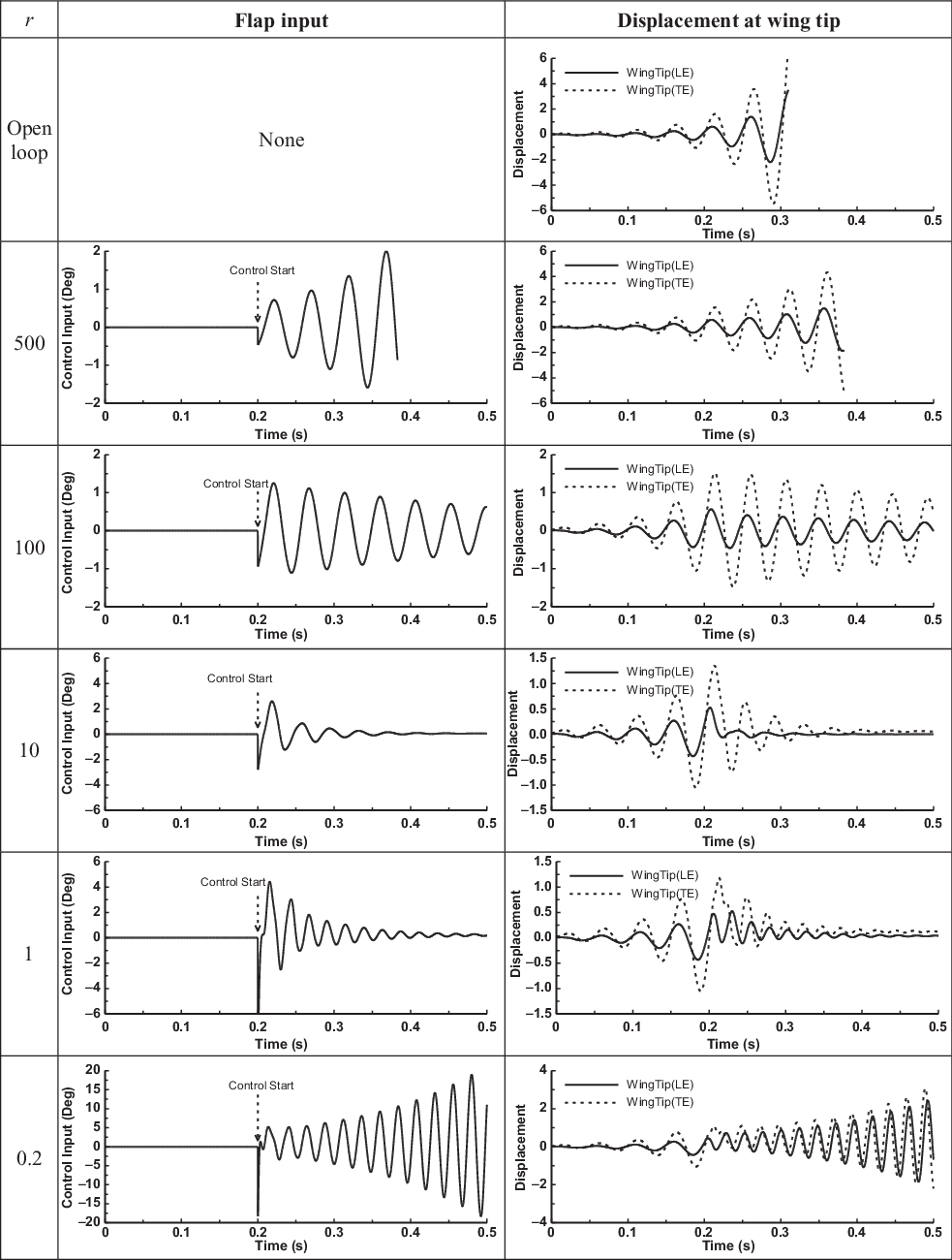
Figure 4. Closed-loop responses for different r values at ${M_\infty } = 0.85$ and ${U_\mu } = 0.44$ .

Initially, the transonic aerodynamic calculations, which use a set of non-dimensional parameters, were performed at a lower value of the flutter speed index ${U_\mu } = 0.44$ than the actual matched point value of ${U_\mu } = 0.67$ . Computations of both the control laws and the TSD aerodynamics were repeated for a range of cruise Mach numbers from 0.5 to 0.95. The results obtained in the open- and closed-loop cases were qualitatively similar to those of Lai and Lum^{(Reference Lai and Lum49)}, who presented a flutter prediction approach using a combination of full-order computational aeroelastic techniques and reduced-order modelling methods, which were applied to closed-loop and nonlinear Hopf bifurcation analysis of the benchmark transonic aeroelastic AGARD 445.6 wing.

Under transonic flow conditions, high-aspect-ratio wings can exhibit Limit-Cycle Oscillations (LCOs). Trailing-edge flaps can exhibit transonic buzz, an instability driven by aerodynamic nonlinearities. Control surface buzz is an LCO type of aeroelastic instability observed in trailing-edge control surfaces^{(Reference Dowell, Edwards and Strganac50)}. However, Allen et al.^{(Reference Allen, Jones, Taylor, Badcock, Woodgate, Rampurawala, Cooper and Vio51)} confirmed that the calculations of the flutter instability boundaries of the AGARD 445.6 wing based on linear analysis techniques provided reasonably accurate results because of the simplicity of the planform shape. Thus, from the responses obtained numerically, the range of r values for which one could expect closed-loop stability at a desired value of the cruise Mach number are determined.

Now, it is possible to focus on a lower range of values of the relative weighting parameter r and increase the value of the flutter speed index ${U_\mu }$ . The closed-loop flap and wing responses obtained for different r values at the typical nominal cruise Mach number of ${M_\infty } = 0.85$ and a flutter speed index ${U_\mu } = 0.66$ are compared in Fig. 5. An optimum choice is $r \approx 1$ , which implies that the magnitudes of both the modal amplitudes and the flap deflections are of equal importance in the cost function.

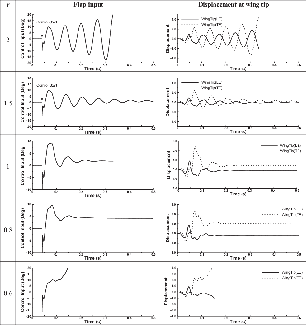
Figure 5. Closed-loop flap and wing responses for different r values at ${M_\infty } = 0.85$ and ${U_\mu } = 0.66$ .

The closed-loop flutter point, with the initial control law computed as explained above and with $r = 1$ , is now established. The Mach number at the onset of flutter, corresponding to the matched flutter point, is just over ${M_\infty } = 0.85$ , corresponding to a flutter speed index of ${U_\mu } = 0.67$ , which is only marginally higher than in Fig. 5. The open- and closed-loop matched point responses at ${M_\infty } = 0.6$ and ${M_\infty } = 0.85$ , respectively, are compared in Fig. 6. Also shown in Fig. 7 are plots of the flutter speed index and the flutter frequency versus the Mach number. The open-loop results are compared with the experimental results of Yates^{(Reference Yates45)} and the results obtained by Lee-Rausch and Batina^{(Reference Lee-Rausch and Batina52)} using the numerical solution of the Euler equations.

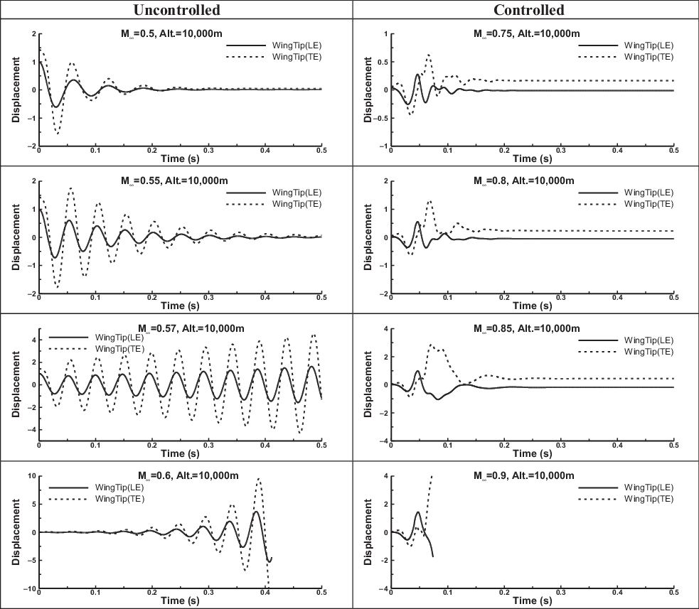
Figure 6. Open and closed-loop responses for $r = 1$ .

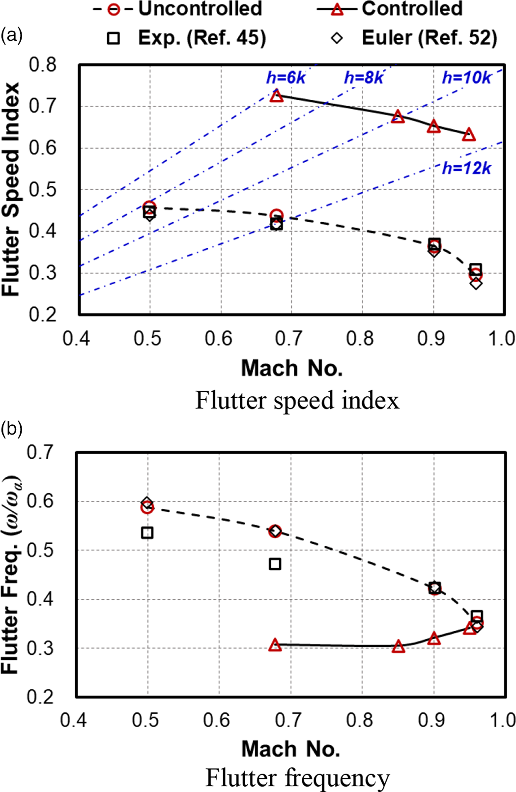
Figure 7. (a) Flutter speed index and (b) flutter frequency versus the Mach number.

The second example considered is the CRM three-dimensional wing with a free stream Mach number ranging from ${M_\infty } = 0.65$ to ${M_\infty } = 0.96$ . Initially, 20 modes were used to perform the flutter analysis. The non-dimensional flutter speed was computed. The number of modes used was reduced to 18, and the non-dimensional flutter speed was re-computed. There was no perceptible change in the flutter speed, which meant that the higher modes did not play a role in determining the flutter speed. This process was continued, and the optimum set of modes to describe the open-loop dynamics was then established. After analysing with several other modal combinations as well, it was decided that the first eight modes were adequate for the synthesis of the control laws. These modes and their shapes are shown in Fig. 8. The open-loop flutter boundaries with a structural damping factor of $g = 0.03$ are compared with the closed-loop flutter boundaries in Fig. 9. The frequencies are reported in Hz for ease of comparison with the modes in Fig. 8 and as reported in ref. ^{(Reference Rivers47)}.

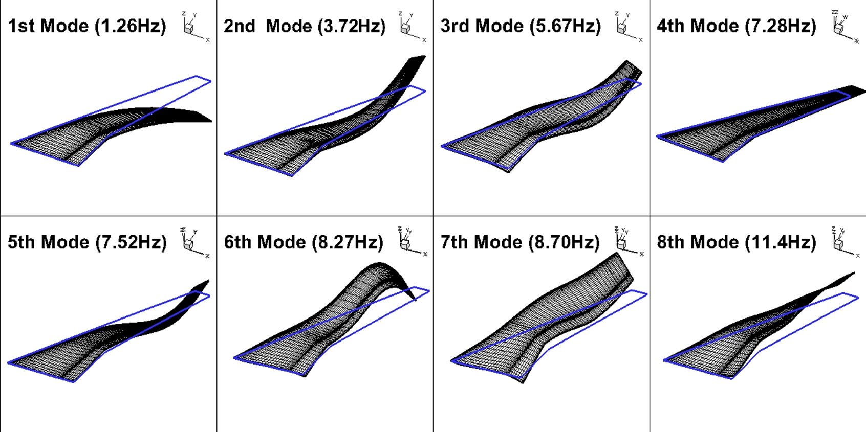
Figure 8. Structural mode shapes and frequencies of the CRM wing-box v15 model.

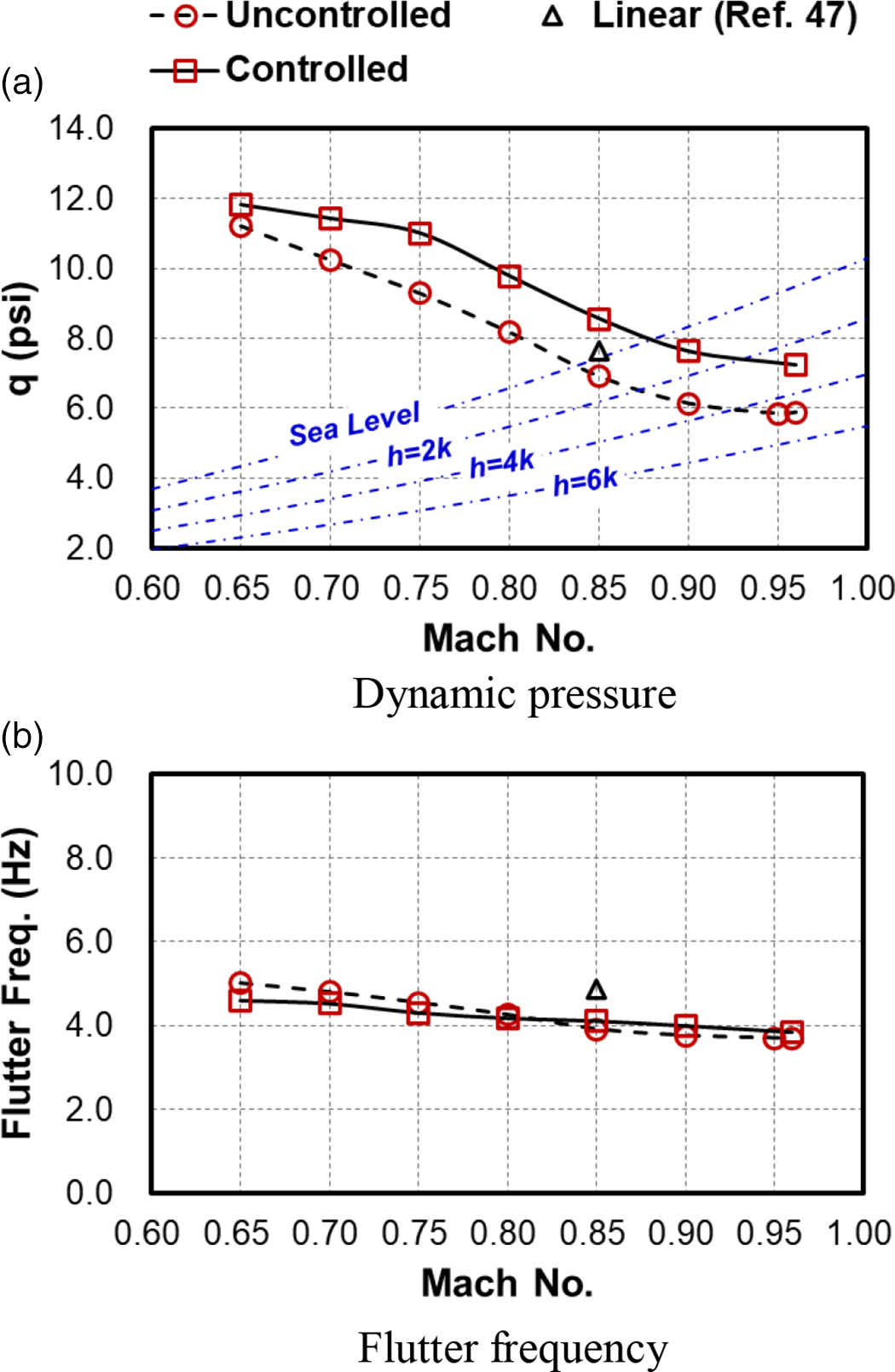
Figure 9. Plots of the open- and closed-loop (a) flutter dynamic pressure and (b) flutter frequency versus the Mach number for the CRM planform.

The initial set of control law gains for the 16 states in the model were first computed for several free stream Mach numbers given by, ${M_\infty } = 0.65, \cdots ,{\rm{ }}0.85,0.88,0.90, \cdots ,0.96$ , and for $r$ values ranging from 1 to 10, representing over 200 gain vector sets to facilitate a wide search. The lowest gain magnitudes were obtained for ${M_\infty } = 0.65$ with $r = 10$ , and the highest for ${M_\infty } = 0.96$ with $r = 1$ . A systematic search amongst these gain vector sets was then performed to identify the best gain vector sets, both in terms of optimality and to ensure feasibility of physical implementation, using the nonlinear TSD aerodynamics to compute the closed-loop characteristics. After establishing the trends in the changes in the flutter speeds, the search was restricted to a much smaller number of selected gain vector sets.

The closed-loop computations were performed over a much larger time frame as compared with the earlier example, with a similar time step, as the frequencies of vibration were significantly smaller in this example. So, the computations took much longer. The closed-loop response computations and analysis were also performed for ${M_\infty } = 0.65, \cdots ,{\rm{ }}0.96$ . Since the CRM is a high-aspect-ratio wing, it is important to ensure that the occurrence of control surface buzz of the LCO type is avoided. Figure 10 compares the open- and closed-loop responses of the wing at ${M_\infty } = 0.85 - 0.96$ with $r = 1$ and with a dynamic pressure equal to q = 6.52 psi to 7.17psi. The increase in the closed-loop flutter speed is more than 16%. Increasing the r value from 1 to about 5 did not have a significant effect on the closed-loop flutter speed. Thus, the key feedbacks and modal quantities could be identified.

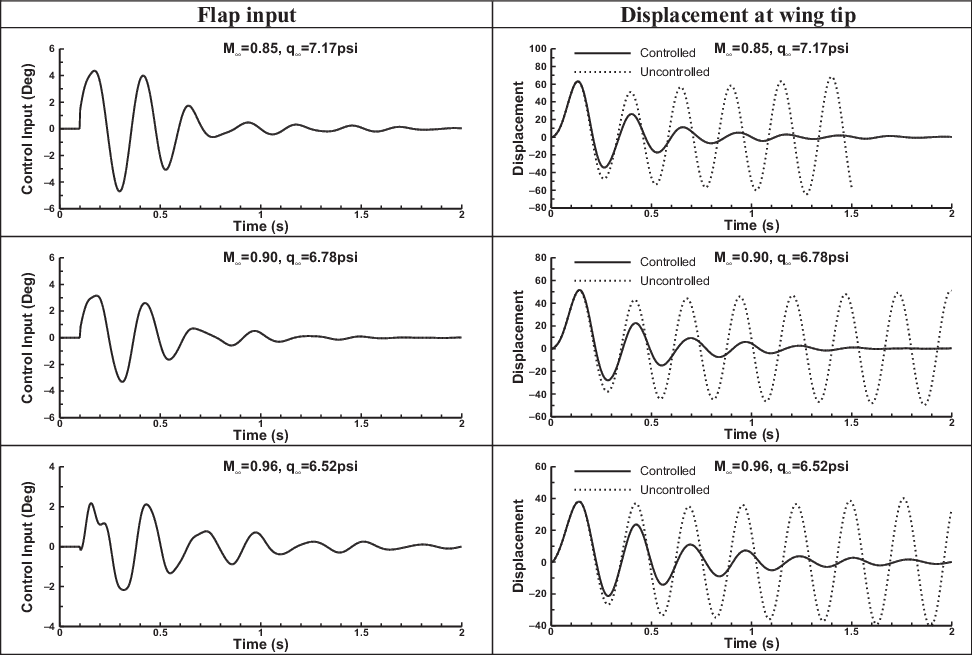
Figure 10. Comparison of open- and closed-loop responses at ${M_\infty } = 0.85,{\rm{ 0}}{\rm{.90, 0}}{\rm{.96}}$ with $r = 1$ .