Nomenclature
-
 $ C_D$
-
Coefficient of drag
-
$ C_{D, diffuse}$
-
Coefficient of drag for diffuse reflection from surface
-
$C_T $
-
Coefficient of torque
-
$\vec{a} $
-
Sum of all perturbing accelerations
-
$ a_0$
-
Semi-major axis of an orbit
-
$ a_d$
-
Drag deceleration
-
$A $
-
Cross-sectional area of a spacecraft
-
$A_e $
-
Effective cross-sectional area of a spacecraft
-
$\vec{D} $
-
Drag force
-
$\vec{F} $
-
Resultant aerodynamics force
-
$I_z $
-
Moment of inertia about z axis
-
$\vec{L} $
-
Lift force
-
$ \vec{L}_0$
-
Characteristic length of spacecraft
-
$ m$
-
Mass of a spacecraft
-
$p $
-
Orbital time period
-
$ r$
-
Magnitude of position vector
-
$ \vec{r}$
-
Position vector of a spacecraft measured from centre of attracting body
-
$\ddot{\vec{r}} $
-
Acceleration experienced by a spacecraft
-
$S $
-
Speed ratio
-
$S_w $
-
Speed ratio based on wall temperature
-
$ \vec{T}$
-
Torque
-
$ \vec{T}_z$
-
Pitching torque about z axis
-
$ {T}_\infty$
-
Free stream temperature
-
$U $
-
Free stream speed
-
$ v_R$
-
Magnitude of spacecraft velocity relative to atmosphere
-
$ \hat{v}_{R }$
-
Unit vector along spacecraft relative velocity
-
$ \alpha$
-
Angle of attack
-
$ \beta$
-
Ballistic coefficient
-
$ \delta \vec{d}$
-
Position vector of centre of pressure from centre of mass
-
$ \delta x$
-
X component of position vector of centre of pressure from leading edge
-
$\delta y $
-
Y component of position vector of centre of pressure from leading edge
-
$\lambda $
-
Mean free path
-
$\mu $
-
Standard gravitational parameter
-
$ \omega$
-
Angular velocity
-
$ \rho$
-
Density
-
$\rho_\infty $
-
Free stream density


Abbreviations
- CLL
-
Cercignani-Lampis-Lord
- CM
-
Centre of mass
- CP
-
Centre of pressure
- DSMC
-
Direct Simulation Monte Carlo
- LEO
-
Low Earth Orbit
1.0 Introduction
Space exploration began with the launch of the first artificial satellite, Sputnik, by the Soviet Union in 1957. Since then, numerous missions and crewed spacecraft have been launched for various purposes. All of these spacecrafts have contributed to the increasing population of “space debris”, which refers to both natural debris (asteroids, comets and meteoroids) and artificial/orbital debris (old satellites and spent rocket stages). Spacecraft are thus exposed to the risk of collision with on-orbit debris and operational satellites [Reference Rossi and Valsecchi1]. This risk is particularly significant in Low Earth Orbit (LEO), where the majority of space debris is present. The increasing population of space debris and the various hazards it poses are discussed in Ref. [Reference Meja-Kaiser2]. A naturally decaying satellite might contribute to long-lasting debris for years if on-orbit collisions happen with objects in a low-perigee elliptical orbit [Reference Omar and Bevilacqua3]. Collisions of space debris with a functional spacecraft can damage its hardware and populate the orbit with additional debris, further increasing the complications of future space missions [Reference Liou, Matney, Vavrin, Manis and Gates4, Reference Kessler and Cour-Palais5]. Due to its high velocity, even small debris measuring 1–10cm can cause catastrophic damage to operational satellites on collision. Future spacecrafts must avoid such accidents by collision avoidance manoeuvres [Reference Yehia6]. Standard debris mitigation practices demand accurate information about its position and motion, that is, the trajectory of a spacecraft in LEO, to avoid collisions with orbital debris and other working satellites, and to reduce human casualties in case of re-entry into Earth’s atmosphere.
The orbit of a satellite in LEO will decay due to the damping effect of the rarified atmosphere at hypersonic speed, such that the satellite experiences a gradual decrease in altitude. As a result of this orbital decay, objects in space will de-orbit and re-enter Earth’s atmosphere in either a controlled or uncontrolled manner [Reference Grossir, Puorto, Ilich, Paris, Chazot, Rumeau, Spel and Annaloro7]. Every year, on average, 100 human-made objects de-orbit and re-enter the atmosphere. Some cases of actual re-entry can be found in past works [Reference King-Hele and Walker8, Reference King-Hele, Walker and Neirinck9]. Many fragments of these de-orbited spacecrafts and debris survive re-entry and impact with the ground; the Skylab and Cosmos 954 spacecraft are such examples [Reference King-Hele and Walker8, Reference King-Hele, Walker and Neirinck9]. Falling satellites may pose a risk to humans, aircraft and other objects. Hence, to reduce the risk of on-ground casualties and to calculate the ground impact area and impact time of such satellites, information about re-entry trajectories and flow properties that influence the survivability of debris are required [Reference Grossir, Puorto, Ilich, Paris, Chazot, Rumeau, Spel and Annaloro7, Reference Monogarov, Melnikov, Drozdov, Dilhan, Frolov, Muravyev and Pivkina10, Reference Liang, Li, Li and Shi11, Reference Li, Peng, Ma, Dang, Tang and Sun12].
In the work by Liang et al. [Reference Liang, Li, Li and Shi11], the DSMC method was used to predict the heating rate, pressure distribution and the structural stress of a spacecraft during re-entry. The atmospheric disintegration and ablation were predicted to accurately estimate the debris spread area. Li et al. [Reference Li, Peng, Ma, Dang, Tang and Sun12] used a dynamic thermo-mechanical coupling model to study the disintegration of the metal truss structure of a spacecraft falling into Earth’s atmosphere in an uncontrolled manner. Uncontrolled falling space objects may disintegrate into many bodies, necessitating the study of multi-body interactions in a re-entry flow situation. The multi-body flow interference among hypersonic re-entering objects flying side-by-side was studied by Li et al. [Reference Li, Peng, Ma, Dang, Tang and Sun12] and Peng et al. [Reference Peng, Li, Wu and Jiang13]. A computational tool required for dynamically coupled analysis of the thermoelasticity, deformation and stresses of a body under such an aero-thermodynamic re-entry environment was developed by Li et al. [Reference Li, Ma and Cui14].
In LEO, a spacecraft experiences aerodynamic forces and torques due to the presence of an extremely rarefied atmosphere. The Knudsen number, Kn, that is, the ratio of the mean free path of a gas to a characteristic length, can become very large, on the order of several hundred. Aerodynamic torque causes the spacecraft to tumble throughout the LEO, because of which they are sometimes called tumbling bodies [Reference De-Lafontaine and Garg15, Reference De-Lafontaine and Garg16]. Orbital decay and tumbling occur simultaneously throughout the LEO due to these forces. The drag force is the primary source of perturbation in LEO, since the order of magnitude of the perturbation caused by drag is much larger compared with other orbital perturbations [Reference De-Lafontaine and Garg16]. Therefore, it is essential to predict the aerodynamic forces and torques experienced by orbiting and re-entering spacecrafts or space debris to estimate the orbital perturbation and thereby the trajectory of spacecraft.
The lifetime of an object orbiting in LEO is affected by various perturbations, which ultimately lead to re-entry into Earth’s atmosphere. Various studies have been carried out on orbital decay and lifetime analysis over the past few decades [Reference Park, Kim and Park17, Reference Sterne18, Reference Liu and Alford19, Reference Chao and Platt20, Reference Dutt and Anilkumar21, Reference Cefola, Phillion and Kim22, Reference Afful23, Reference San-Juan, San-Martn, Pérez and López24]. Knowledge regarding the position and velocity of orbiting objects becomes necessary for orbit prediction. In literature, the techniques applied to solve such perturbation problems can be classified into three classical approaches: general perturbation, special perturbation and semi-analytic [Reference San-Juan, San-Martn, Pérez and López24, Reference Vallado25]. The general perturbation method can be used to obtain an analytical solution. This method depends on a series expansion of the perturbation equations. However, the accuracy of such analytical solutions is usually low because only the most relevant perturbations can be taken into consideration by such a low-order approximation of a series expansion, although these methods are computationally efficient [Reference Park, Kim and Park17]. Special perturbation techniques use numerical integration to solve the equation of motion with perturbations. This technique offers higher accuracy as compared with a general perturbation method, since it uses complex perturbation models. However, its computational efficiency is low because of the small integration steps applied [Reference Park, Kim and Park17]. The semi-analytical technique relies on a combination of both general and special perturbation techniques to achieve both accuracy and efficiency [Reference Park, Kim and Park17, Reference San-Juan, San-Martn, Pérez and López24]. Recent studies performed using semi-analytical techniques have shown good agreement with existing data [Reference Afful23]. In recent years, several attempts to accurately predict orbital lifetimes have been made using hybrid perturbation theory or the probabilistic assessment method [Reference San-Juan, San-Martn, Pérez and López24, Reference Dell’Elce, Arnst and Kerschen26]. Hybrid perturbation theory is a combination of integration and prediction based on statistical time series [Reference San-Juan, San-Martn, Pérez and López24], whereas the probabilistic assessment method considers the modelling errors in lifetime estimation as well as the primary sources of uncertainties, such as the initial position of the debris, the atmospheric drag and other physical properties [Reference Dell’Elce, Arnst and Kerschen26].
Space debris mitigation standards have been established to limit the risk posed by re-entering space objects, thereby reducing the probability of on-ground casualties [Reference Kato27]. Orbital decay and re-entry prediction of orbiting objects is an ongoing process since it requires tracking of the object to acquire its real-time position and motion. Therefore, computer programs to perform such numerical integration become essential to increase the accuracy of such predictions while reducing the computation time required [Reference Park, Kim and Park17]. Several computer codes developed by various space agencies and research centres for monitoring orbiting objects were reviewed in Ref. [Reference Park, Kim and Park17].
Such numerical codes can primarily be classified into two categories: objected-oriented codes and spacecraft-oriented codes. Most of these codes are deterministic, but to account for the uncertainties involved in the re-entry process, some codes also apply probabilistic approaches [Reference Frank, Weaver and Baker28, Reference Wu, Hu, Qu, Wang and Wu29]. The Object Reentry Survival Analysis Tool (ORSAT) was developed by the National Aeronautics and Space Administration (NASA) [Reference Rochelle, Kinsey, Reid, Reynolds and Johnson30]. It is a deterministic object-oriented computer code used by NASA primarily for the prediction of the re-entry survivability of satellites re-entering from orbital decay or via controlled entry. For a similar purpose, the European Space Agency (ESA) developed a spacecraft-oriented deterministic re-entry code called Spacecraft Atmospheric Reentry and Aerothermal Breakup (SCARAB) [Reference Lips, Fritsche, Koppenwallner and Klinkrad31]. Both the ORSAT and SCARAB codes are well validated for simple shapes and are typically used for orbital object re-entry predictions [Reference Choi, Cho, Lee, Kim and Jo32]. A few open-source programs are also available for orbital decay analysis, such as Debris Risk Assessment and Mitigation Analysis (DRAMA) from ESA and Debris Assessment Software (DAS) by NASA. These open-source codes are easily accessible and available to the public but suffer from certain limitations, in comparison with ORSAT and SCARAB, arising from the models and assumptions used in them [Reference Lips and Fritsche33]. There are other tools that employ local panel inclination methods for describing spacecraft aerodynamics, such as Debris Reentry and Ablation Prediction System (DRAPS), which is a deterministic object-oriented program developed by Wu et al. [Reference Wu, Hu, Qu, Wang and Wu29]; Simplified Aerothermal Model (SAM) [Reference Merrifield, Beck, Markelov and Molina34], ORSAT-J, a modified version of the NASA ORSAT, developed by the National Space Development Agency of Japan (NASDA) [Reference Lips and Fritsche33], Survivability Analysis Program for Atmospheric Reentry (SAPAR) by Sim and Kim [Reference Sim and Kim35] and Free Open Source Tool for Reentry Asteroids and Debris (FOSTRAD) [Reference Mehta, Minisci, Vasile, Walker and Brown36]. To the best of the authors’ knowledge, most of the above-mentioned tools adopt a simplified (low-fidelity) aerodynamic approach: either they assume
 $C_{D}$
to be constant for the orbital decay analysis or they do not consider an accurate variation of
$C_{D}$
to be constant for the orbital decay analysis or they do not consider an accurate variation of
 $C_{D}$
with respect to a number of variables, including the shape, motion, angle-of-attack, ambient gas composition, etc. [Reference De-Lafontaine and Garg15, Reference Lips and Fritsche33].
$C_{D}$
with respect to a number of variables, including the shape, motion, angle-of-attack, ambient gas composition, etc. [Reference De-Lafontaine and Garg15, Reference Lips and Fritsche33].
The aim of the work presented herein is to include the variation of the aerodynamic coefficients with respect to the shape, motion and angle-of-attack of a spacecraft using the DSMC approach. In this work, in-house solvers are used to incorporate the variation of
 $C_{D}$
with the aforesaid parameters when performing a realistic orbital decay analysis. Since dynamic calculation of the aerodynamic coefficients using the DSMC method is very expensive, we pre-calculate their variation over a broad range of speed and angle-of-attack using our in-house DSMC solver, modified to work efficiently in the free molecular regime [Reference Chinnappan, Kumar, Arghode, Kammara and Levin37, Reference Chinnappan, Kumar and Arghode38]. The aerodynamic coefficients thus calculated are used as a look-up table for an orbital decay simulation to study the decay trajectory for space vehicles in LEO by numerically integrating the orbital dynamics equation. Two case studies on two sample bodies (a sphere and an Apollo space capsule) are presented, having different geometrical specifications (in terms of shape and size), so that the effects of geometrical parameters on the orbital decay trajectory can be analysed. The sphere is chosen because it allows a comparison of the simulation results with theory in the free molecular regime. On the other hand, the Apollo space capsule is chosen as a realistic geometry for a space capsule for analysis as space debris re-entering Earth’s atmosphere. The tumbling motion of the orbiting body during its orbital decay in LEO is also considered.
$C_{D}$
with the aforesaid parameters when performing a realistic orbital decay analysis. Since dynamic calculation of the aerodynamic coefficients using the DSMC method is very expensive, we pre-calculate their variation over a broad range of speed and angle-of-attack using our in-house DSMC solver, modified to work efficiently in the free molecular regime [Reference Chinnappan, Kumar, Arghode, Kammara and Levin37, Reference Chinnappan, Kumar and Arghode38]. The aerodynamic coefficients thus calculated are used as a look-up table for an orbital decay simulation to study the decay trajectory for space vehicles in LEO by numerically integrating the orbital dynamics equation. Two case studies on two sample bodies (a sphere and an Apollo space capsule) are presented, having different geometrical specifications (in terms of shape and size), so that the effects of geometrical parameters on the orbital decay trajectory can be analysed. The sphere is chosen because it allows a comparison of the simulation results with theory in the free molecular regime. On the other hand, the Apollo space capsule is chosen as a realistic geometry for a space capsule for analysis as space debris re-entering Earth’s atmosphere. The tumbling motion of the orbiting body during its orbital decay in LEO is also considered.
2.0 Computational model
As mentioned above, the present work focusses on the calculation of the aerodynamics forces and moments on an orbiting, non-operational spacecraft, followed by its dynamics during its orbital decay. Therefore, the computational model developed herein primarily involves two models: an aerodynamics model to calculate the aerodynamic forces/torques, and an orbital dynamics model to simulate the orbital decay of the space vehicle. The aerodynamic model is used to calculate the drag and torque coefficients, which are then applied in the dynamics model for the orbital decay simulation. This section includes an explanation of the aerodynamics model, including the calculation of the drag and torque coefficients in the DSMC-based framework, and the orbital mechanics and methodology for the orbital decay simulation.
2.1 Aerodynamics model
Due to the high degree of rarefaction at high altitudes, the kinetic particle-based DSMC method is highly suitable for the calculation of the aerodynamics forces and torques on an orbiting spacecraft. This method proposed by Bird [Reference Bird39] provides a physics-based solution to the Boltzmann equation by mimicking the behaviour of molecules but without directly solving the Boltzmann equation. The DSMC method uses simulated molecules, each of which represents a cluster of actual molecules. In the DSMC approach, the behaviour of the molecules is modelled through their movement and intermolecular collisions. Their movement is modelled in a deterministic manner, whereas intermolecular collisions are modelled probabilistically. The primary assumption of the DSMC approach is that the movement and intermolecular collisions can be decoupled over a small time interval. DSMC simulation results have also been proven to converge towards solutions of the Boltzmann equation in the limit of an infinite number of particles, for a cell size smaller than the mean free path and a time step smaller than the mean collision time [Reference Bird39]. A proof of the convergence of the DSMC method and the Gas-Kinetic Unified Algorithm (GKUA) for the Boltzmann equation was investigated in the work of Li et al. [Reference Li, Fang, Jiang and Wu40]. The DSMC method can be used in all flow regimes in the dilute gas framework, but is primarily used in the rarefied and free molecular regime (Kn
 $ > 0.1$
) due to its computational efficiency. Moreover, the development and application of coupled Navier–Stokes/DSMC solvers to simulate hypersonic flows in the transitional flow regime and multi-component plume flows from satellite attitude-control engines have been extensively reviewed in the work of Li et al. [Reference Li, Li, Wu and Peng41]. Furthermore, Li et al. [Reference Li, Cai and Li42] studied low-speed microchannel rarefied flows using the direct simulation Bhatnagar–Gross–Krook (DSBGK) model equation, also discussing the limitations associated with the use of the DSMC method to study such problems. A detailed explanation of the DSMC method can be found in Ref. [Reference Bird39].
$ > 0.1$
) due to its computational efficiency. Moreover, the development and application of coupled Navier–Stokes/DSMC solvers to simulate hypersonic flows in the transitional flow regime and multi-component plume flows from satellite attitude-control engines have been extensively reviewed in the work of Li et al. [Reference Li, Li, Wu and Peng41]. Furthermore, Li et al. [Reference Li, Cai and Li42] studied low-speed microchannel rarefied flows using the direct simulation Bhatnagar–Gross–Krook (DSBGK) model equation, also discussing the limitations associated with the use of the DSMC method to study such problems. A detailed explanation of the DSMC method can be found in Ref. [Reference Bird39].
For this work, the parallel, in-house, multi-species DSMC solver named Non-equilibrium Flow Solver (NFS) [Reference Kumar and Chinnappan43], which is based on Bird’s DSMC algorithm, is modified to develop a computationally efficient DSMC-based solver for free molecular flow [Reference Chinnappan, Kumar, Arghode and Myong44]. The modifications made to the DSMC algorithm are consistent with the assumption of free molecular flow. First, intermolecular collisions are not modelled in the modified DSMC solver, since the gas flow is assumed to be collisionless in the free molecular flow regime. Second, after the gas–surface interaction model calculations are performed for the interaction of a gas particle with a surface, its velocity is then assigned the same value as before the collision and it is relocated randomly inside the domain. This is to ensure that the incident gas remains unaffected by the presence of body, which is consistent with the assumptions made in free molecular flow theory [Reference Chambre and Schaaf45]. Thus, the core of the modified DSMC solver consists of initialisation, particle movement, gas–surface interaction and sampling of surface properties. A detailed explanation related to the algorithm of the solver can be found in Chinnappan et al. [Reference Chinnappan, Kumar, Arghode and Myong44].
2.2 Calculation of drag and torque
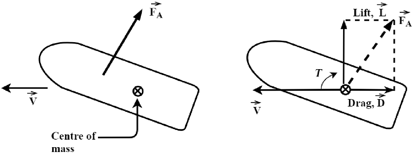
Aerodynamic forces are the main non-gravitational forces acting on a satellite due to the presence of the rarefied atmosphere in LEO. These forces can be resolved as follows (Fig. 1):
The drag force is a non-conservative force [Reference Vallado25] acting in the direction opposite to the satellite’s velocity vector, thereby resulting in energy dissipation from the orbit of the satellite. The dissipation of energy slows down the spacecraft, which then leads to orbital decay. The drag and lift forces are calculated in the DSMC framework by integrating the pressure and shear stress distribution around the body. The lift force is another part of the aerodynamic force, acting in a direction normal to the relative velocity vector. It is worth noting that there is no resultant lift acting on a satellite exhibiting uncontrolled tumbling motion, which is a valid assumption since the effect of the lift force is averaged out over its lifetime [Reference Cook46]. Thus, in the present work on the orbital decay analysis of a tumbling body, only the perturbation due to the drag force and the effect of the tumbling motion are considered. Moreover, it is shown below that the magnitude of the lift force is much smaller as compared with the drag force.
A spacecraft undergoes tumbling motion throughout its orbit [Reference De Pontieu47]. In the present work, the influence of the aerodynamic forces and torques on the tumbling motion is examined. The in-house modified DSMC solver, as explained above, is used to calculate the aerodynamic properties of the spacecraft. The aerodynamic forces (F) are obtained by integrating the pressure and shear stress over the surface of the spacecraft. These aerodynamic forces act around the Centre of Mass (CM), producing a torque. The torque caused by the aerodynamic forces can bes calculated using the analytical expression
 $\vec{T}= \delta \vec{d}\times \vec{F}$
, where
$\vec{T}= \delta \vec{d}\times \vec{F}$
, where
 $\delta\vec{d}$
is the position vector of the centre of pressure (CP) from the CM, and
$\delta\vec{d}$
is the position vector of the centre of pressure (CP) from the CM, and
 $\vec{F}$
is the resultant aerodynamic force acting on the body, as shown in Fig. 2. The lift (L) and drag (D) forces are the x and y components of the resultant force vector, respectively. To simplify this problem, we consider only one-dimensional rotation of a spacecraft about its pitching axis (z-axis) to model the tumbling motion, as illustrated in Fig. 2.
$\vec{F}$
is the resultant aerodynamic force acting on the body, as shown in Fig. 2. The lift (L) and drag (D) forces are the x and y components of the resultant force vector, respectively. To simplify this problem, we consider only one-dimensional rotation of a spacecraft about its pitching axis (z-axis) to model the tumbling motion, as illustrated in Fig. 2.

Figure 1. The aerodynamic forces on a satellite [Reference De-Lafontaine and Garg15].
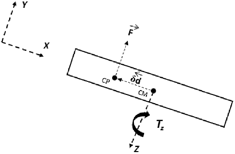
Figure 2. Schematic of a body experiencing torque.
A parameter called the pitching torque coefficient (
 $C_T$
) is defined to normalise the torque acting on the spacecraft:
$C_T$
) is defined to normalise the torque acting on the spacecraft:
 \begin{equation}C_T=\frac{T_z}{\rho U^{2}SL},\end{equation}
where
 $T_z$
is the pitching torque about the z-axis, S is the reference area of the spacecraft and L is its characteristic length.
$T_z$
is the pitching torque about the z-axis, S is the reference area of the spacecraft and L is its characteristic length.
2.3 Orbital dynamics model
Using Newton’s second law and the universal law of gravitation, the equations for the relative motion of two bodies can be derived by assuming them to be point masses:
 \begin{align}\ddot{\vec{r}}+\frac{\mu}{r^{3}}\vec{r}=0,\end{align}
where
 $\vec{r}$
is the position vector of the spacecraft measured from the centre of the attracting body and
$\vec{r}$
is the position vector of the spacecraft measured from the centre of the attracting body and
 $\mu$
is the standard gravitational parameter. Considering Earth as the attracting body, one has
$\mu$
is the standard gravitational parameter. Considering Earth as the attracting body, one has
 $\mu = 3.99\times10^{14}\textit{m}^{3}/\mathrm{s}^{2}$
[Reference Curtis48].
$\mu = 3.99\times10^{14}\textit{m}^{3}/\mathrm{s}^{2}$
[Reference Curtis48].
Equation (2) is the basis of the unperturbed motion of a spacecraft, considering only the gravitational force. In real life, a spacecraft in LEO encounters various forces apart from the gravitational force. These various forces cause perturbations that lead to a deviation of the spacecraft from its ideal orbit. The equation of relative motion of two bodies under such orbital perturbation can be expressed as
 \begin{equation}\ddot{\vec{r}}+\frac{\mu}{r^{3}} \vec{r}=\vec{a},\end{equation}
where
 $\vec{a}$
is the sum of all the perturbing accelerations [Reference Curtis48].
$\vec{a}$
is the sum of all the perturbing accelerations [Reference Curtis48].
In the current study, only the drag perturbation is considered, because for spacecraft in LEO, this perturbation is many times larger than other orbital perturbations [Reference King-Hele49]. The mathematical expression used to model the deceleration due to drag is given by Ref. [Reference Vallado25] as follows:
 \begin{equation}\vec{a}_{d}=-\frac{1}{2}\rho \frac{C_{D} A}{m} v_{R}^{2} {\hat{v}_{R }},\end{equation}
where
 $C_D$
is the drag coefficient,
$C_D$
is the drag coefficient,
 $\rho$
is the density of the atmosphere, A is the cross-sectional area and m is the mass of the satellite,
$\rho$
is the density of the atmosphere, A is the cross-sectional area and m is the mass of the satellite,
 $v_R$
is the magnitude of the satellite’s velocity relative to the atmosphere and
$v_R$
is the magnitude of the satellite’s velocity relative to the atmosphere and
 $\hat{v}_{R }$
is the unit vector along the satellite’s relative velocity. The term
$\hat{v}_{R }$
is the unit vector along the satellite’s relative velocity. The term
 $\frac{m}{C_D A}$
is known as the ballistic coefficient
$\frac{m}{C_D A}$
is known as the ballistic coefficient
 $\beta$
, being a measure of the spacecraft’s susceptibility to drag effects and indicating how fast the orbit of the spacecraft will decay. Spacecraft with low
$\beta$
, being a measure of the spacecraft’s susceptibility to drag effects and indicating how fast the orbit of the spacecraft will decay. Spacecraft with low
 $\beta$
values respond quickly to the atmosphere, and their orbit will decay faster than those with high values of
$\beta$
values respond quickly to the atmosphere, and their orbit will decay faster than those with high values of
 $\beta$
[Reference Wertz, Everett and Puschell50].
$\beta$
[Reference Wertz, Everett and Puschell50].
The orbital decay program is employed to estimate the orbital decay trajectory of a tumbling body. The basis of the orbital decay is Equations (3) and (5) (as given below). Equation (3) describes the relative motion of two bodies under orbital perturbations. In the present work, the drag force is the only orbital perturbation considered in the orbital decay analysis. The drag perturbation is modelled using Equation (4). Meanwhile, Equation (5) describes the rotational dynamics of the body and is used to model its tumbling motion, considering only rotation about its z-axis. In Equation (5),
 $\omega$
is the angular momentum and
$\omega$
is the angular momentum and
 $I_z$
is the moment of inertia of the spacecraft about the z-axis.
$I_z$
is the moment of inertia of the spacecraft about the z-axis.
 \begin{align}T_z=I_z\ddot{\alpha}=I_z\dot{\omega}.\end{align}
The computer program for the orbital decay simulation solves Equations (3) and (5) simultaneously. The Earth-Centred Inertial (ECI) coordinate system is employed in the orbital decay simulation. A circular orbit is assumed while developing the computer code. Note that this assumption is made to simplify the analysis to some extent. Figure 3 shows the algorithm of the orbital decay program.
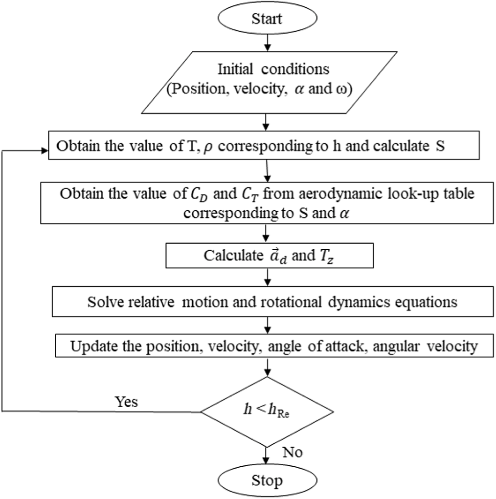
Figure 3. Orbital decay program algorithm.
In Fig. 3, h and
 $h_{\rm Re}$
are the altitude and re-entry altitude of the spacecraft, respectively, from the Earth’s surface. Reentry is assumed to occur when the spacecraft descends to an altitude of 180km [Reference Kennewell51]. After reaching this altitude, the spacecraft will impact within a few hours. The look-up table for the aerodynamics coefficients obtained using the free molecular flow simulation and the US Standard Atmosphere 1976 [52] is used as input to this computer program. Finally, the orbital decay trajectory of the spacecraft is obtained by plotting the altitude of the spacecraft versus time.
$h_{\rm Re}$
are the altitude and re-entry altitude of the spacecraft, respectively, from the Earth’s surface. Reentry is assumed to occur when the spacecraft descends to an altitude of 180km [Reference Kennewell51]. After reaching this altitude, the spacecraft will impact within a few hours. The look-up table for the aerodynamics coefficients obtained using the free molecular flow simulation and the US Standard Atmosphere 1976 [52] is used as input to this computer program. Finally, the orbital decay trajectory of the spacecraft is obtained by plotting the altitude of the spacecraft versus time.
3.0 Solver validation
The validation of the aerodynamics and orbital dynamic models is presented in this section.
3.1 Aerodynamics model validation
The modified DSMC solver is already validated for many flow problems, such as flow over a sphere at low and high speed ratios, and a flat plate at different angles of attack [Reference Chinnappan, Kumar, Arghode and Myong44]. Additionally, we present herein its validation for free molecular flow over a sphere by comparing the simulation results against theory. The validation case study involves flow over a spherical body at different speed ratios. The drag coefficient (
 $C_D$
) is compared with the theoretical expression for the drag experienced by a sphere (with diffuse reflection) in the free molecular flow regime given by Equation (6). Figure 4 shows the computational domain and the mesh employed for the validation case study.
$C_D$
) is compared with the theoretical expression for the drag experienced by a sphere (with diffuse reflection) in the free molecular flow regime given by Equation (6). Figure 4 shows the computational domain and the mesh employed for the validation case study.
 \begin{align}C_{D,{\rm diffuse}}&=\frac{e^{-S^{2}}}{\sqrt{\pi} S^{3}}\left(1+2 S^{2}\right)+\frac{4 S^{4}+4 S^{2}-1}{2 S^{4}} \operatorname{erf}(S)+\frac{2 \sqrt{\pi}}{3 S_{{w}}}\end{align}
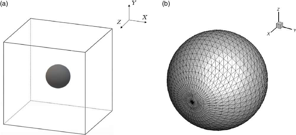
Figure 4. (a) Computational domain. (b) Mesh for a sphere experiencing free molecular flow.
A cubic computational cell is considered with a spherical body at the centre. Periodic boundary conditions are employed on all six sides of the domain. Each simulation is performed with 20,000 simulated particles and 50,000 samples. The time step for the simulation is
 $1\times10^{-10}$
s, chosen such that it is less than the mean collision time of the gas. The Cercignani–Lampis–Lord (CLL) model is used for the gas–surface interaction with entirely diffuse reflection.
$1\times10^{-10}$
s, chosen such that it is less than the mean collision time of the gas. The Cercignani–Lampis–Lord (CLL) model is used for the gas–surface interaction with entirely diffuse reflection.
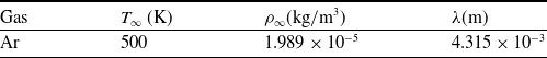
The freestream conditions used for the simulation are presented in Table 1. The wall temperature is kept the same as the freestream temperature.
Table 1. Freestream conditions for free molecular flow simulations over a sphere
The variation of the drag coefficient with the speed ratio is obtained from the in-house modified DSMC solver, as described in Section A. The results are plotted and compared with theory in Fig. 5. It is clearly observed that the
 $C_D$
profile is in excellent agreement with the analytical results over the considered range of speed ratio.
$C_D$
profile is in excellent agreement with the analytical results over the considered range of speed ratio.
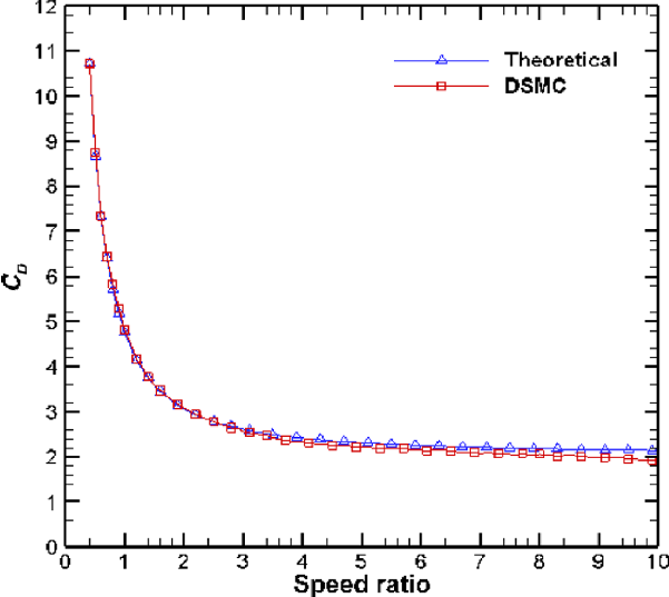
Figure 5. Comparison of DSMC and analytical results for spherical body.
3.2 Orbital decay validation
The orbital decay simulation is validated against a period reduction model given by the Australian IPS Radio and Space Services [Reference Kennewell51]. The governing equation for the period reduction model is expressed as
 \begin{align}\frac{dp}{dt}=-3\pi a\rho \left(\frac{A_e}{m}\right),\end{align}
where P is the orbital time period, m is the mass of the satellite, a is the semi-major axis of its orbit,
 $A_e$
is the effective cross-sectional area, defined as
$A_e$
is the effective cross-sectional area, defined as
 $A_e= A C_D$
with A being the cross-sectional area of the satellite and
$A_e= A C_D$
with A being the cross-sectional area of the satellite and
 $C_D$
is the coefficient of drag experienced. In the period reduction model, drag is the only aerodynamics force taken into account. Equation (7) calculates the reduction in the orbital period in the time step dt by using the current altitude, the atmospheric density and the effective cross-sectional area of the satellite divided by its mass. The period of the orbit is updated, and the new semi-major axis (and hence altitude) of the orbit is calculated as
$C_D$
is the coefficient of drag experienced. In the period reduction model, drag is the only aerodynamics force taken into account. Equation (7) calculates the reduction in the orbital period in the time step dt by using the current altitude, the atmospheric density and the effective cross-sectional area of the satellite divided by its mass. The period of the orbit is updated, and the new semi-major axis (and hence altitude) of the orbit is calculated as
 $a={\left(\frac{p^{2}\mu}{4\pi^{2}}\right)}^{1/3} $
, then the process is repeated until the spacecraft reaches the re-entry altitude of 180km.
$a={\left(\frac{p^{2}\mu}{4\pi^{2}}\right)}^{1/3} $
, then the process is repeated until the spacecraft reaches the re-entry altitude of 180km.
The orbital decay simulation is performed on the same prototypical satellite analysed using the period reduction model in Ref. [Reference Kennewell51]. The prototypical satellite has an effective cross-section
 $A_e = 1\mathrm{m}^{2}$
and mass m = 100kg. The US Standard Atmosphere 1976 [52] is applied to acquire the air density at a given altitude. A starting altitude of 200km is chosen for both simulations.
$A_e = 1\mathrm{m}^{2}$
and mass m = 100kg. The US Standard Atmosphere 1976 [52] is applied to acquire the air density at a given altitude. A starting altitude of 200km is chosen for both simulations.
Figure 6 compares the results obtained from our orbital decay simulation with those of the period reduction model employed on the prototypical satellite. Evidently, the orbital decay trajectory obtained from the orbital decay simulation is in good agreement with the results of the periodic reduction model.
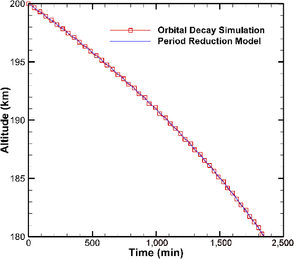
Figure 6. Comparison between orbital decay simulation and periodic reduction model.

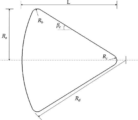
Figure 7. Apollo space capsule geometry [Reference Griffith and Boylan53].
4.0 Main case study: Tumbling body aerodynamics
In the present work, two case studies considering bodies with different geometrical shapes and sizes are considered: a spherical body and the Apollo command module. In the first case study, a sphere of diameter 0.1m and mass 1.2kg is considered, whereas in the second, the Apollo space capsule is chosen, for which the geometrical details are taken from Ref. [Reference Griffith and Boylan53]. The geometry of the Apollo space capsule model chosen for the present study is shown in Fig. 7. The base radius,
 $R_a$
, is 1.956m, the shoulder radius,
$R_a$
, is 1.956m, the shoulder radius,
 $R_b$
, is 0.196m, the cap radius,
$R_b$
, is 0.196m, the cap radius,
 $R_c$
, is 0.232m, the nose radius,
$R_c$
, is 0.232m, the nose radius,
 $R_d$
, is 4.693m, the length of the capsule, L, is 3.621m and the cone angle,
$R_d$
, is 4.693m, the length of the capsule, L, is 3.621m and the cone angle,
 $\beta_c$
, is equal to
$\beta_c$
, is equal to
 $33^{\circ}$
. The total structure and heat shield mass of the Apollo space capsule is 2,410kg.
$33^{\circ}$
. The total structure and heat shield mass of the Apollo space capsule is 2,410kg.
DSMC simulations are performed to obtain a look-up table of the aerodynamic coefficients, which is then applied to perform the orbital decay simulation of the bodies. For the first case study (flow over a sphere), the aerodynamic analysis is presented and discussed over a range of speed ratios in Section A. For a sphere, the only relevant aerodynamic coefficient of importance is the drag coefficient,
 $C_D$
, as shown in Fig. 5. Therefore, in the following, the aerodynamic analysis of the flow over the Apollo space capsule is presented. Later, the orbital decay analysis of the two bodies is compared and discussed.
$C_D$
, as shown in Fig. 5. Therefore, in the following, the aerodynamic analysis of the flow over the Apollo space capsule is presented. Later, the orbital decay analysis of the two bodies is compared and discussed.
For the second case study (the Apollo space capsule), DSMC simulations are performed for a range of speed ratios from 8 to 10 in steps of 0.1, and for angles of attack ranging from
 $0^\circ$
to
$0^\circ$
to
 $90^\circ$
in steps of
$90^\circ$
in steps of
 $2^\circ$
. The range of speed ratio chosen for this study corresponds to the variation of the orbital speed during the orbital decay analysis from 200 to 180km considered in this work. The look-up table contains the variation of
$2^\circ$
. The range of speed ratio chosen for this study corresponds to the variation of the orbital speed during the orbital decay analysis from 200 to 180km considered in this work. The look-up table contains the variation of
 $C_L$
,
$C_L$
,
 $C_D$
and
$C_D$
and
 $C_T$
for a range of speed ratios and angles of attack. The free stream temperature and number density are taken to be 500K and
$C_T$
for a range of speed ratios and angles of attack. The free stream temperature and number density are taken to be 500K and
 $3 \times 10^{20} \frac{1}{{\rm m}^3}$
, corresponding to free molecular conditions. In total, 0.1m simulated particles are used and 1m samples are taken to determine the aerodynamic coefficients. In this work, we consider fully diffuse reflection (corresponding to a tangential accommodation coefficient of unity) on the surface at a temperature of 500K.
$3 \times 10^{20} \frac{1}{{\rm m}^3}$
, corresponding to free molecular conditions. In total, 0.1m simulated particles are used and 1m samples are taken to determine the aerodynamic coefficients. In this work, we consider fully diffuse reflection (corresponding to a tangential accommodation coefficient of unity) on the surface at a temperature of 500K.
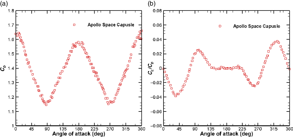
Figure 8 shows the variation of the aerodynamic coefficients with the angle-of-attack,
 $\alpha$
, for the Apollo space capsule at a speed ratio of 10. It is observed from Fig. 8(a) that the
$\alpha$
, for the Apollo space capsule at a speed ratio of 10. It is observed from Fig. 8(a) that the
 $C_D$
of the Apollo space capsule first decreases with the angle-of-attack,
$C_D$
of the Apollo space capsule first decreases with the angle-of-attack,
 $\alpha$
, then reaches a minimum value, and then increases. This occurs because the projected area of the body perpendicular to the flow decreases with
$\alpha$
, then reaches a minimum value, and then increases. This occurs because the projected area of the body perpendicular to the flow decreases with
 $\alpha$
up to
$\alpha$
up to
 $90^{\circ}$
but then increases with further increase in
$90^{\circ}$
but then increases with further increase in
 $\alpha$
, whereas for the case of a sphere, the variation of
$\alpha$
, whereas for the case of a sphere, the variation of
 $C_D$
with angle-of-attack is not applicable. It can be inferred from Fig. 8(b) that the magnitude of
$C_D$
with angle-of-attack is not applicable. It can be inferred from Fig. 8(b) that the magnitude of
 $C_L/C_D$
is always less than 0.05 for the Apollo space capsule. This shows that the order of magnitude of the lift force is significantly smaller than that of the drag force. According to King-Hele [Reference King-Hele49], the lift force can be neglected if
$C_L/C_D$
is always less than 0.05 for the Apollo space capsule. This shows that the order of magnitude of the lift force is significantly smaller than that of the drag force. According to King-Hele [Reference King-Hele49], the lift force can be neglected if
 $C_L/C_D < 0.1$
. For the case of a sphere, it is obvious that the value of
$C_L/C_D < 0.1$
. For the case of a sphere, it is obvious that the value of
 $C_L$
is always zero. Considering this, the lift force is neglected in the orbital decay analysis in the present work.
$C_L$
is always zero. Considering this, the lift force is neglected in the orbital decay analysis in the present work.

Figure 8. Variation of aerodynamic parameters with angle-of-attack for Apollo space capsule at a speed ratio of 10. (a) Drag coefficient. (b) Lift to drag coefficient ratio.
Figure 9 shows the variation of the torque coefficient,
 $C_T$
, with
$C_T$
, with
 $\alpha$
for the Apollo space capsule. It can be seen that the torque coefficient,
$\alpha$
for the Apollo space capsule. It can be seen that the torque coefficient,
 $C_T$
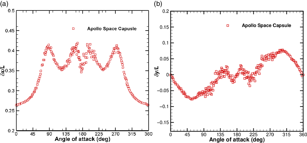
, experienced by the body is mainly dictated by the moment created by the drag force. This is because the magnitude of the lift force is much smaller than that of the drag force, as discussed above. Figure 10(a) and (b) show the x and y components of the position vector of the centre of pressure (CP) of the Apollo space capsule measured from the leading edge.
$C_T$
, experienced by the body is mainly dictated by the moment created by the drag force. This is because the magnitude of the lift force is much smaller than that of the drag force, as discussed above. Figure 10(a) and (b) show the x and y components of the position vector of the centre of pressure (CP) of the Apollo space capsule measured from the leading edge.
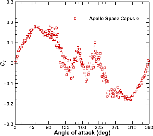
Figure 9. Variation of torque coefficient with angle-of-attack of the Apollo space capsule at a speed ratio of 10.

Figure 10. Position vector of CP with respect to the leading edge. (a) x-component of position vector. (b) y-component of position vector.
For the Apollo space capsule, the value of
 $\delta x$
, as shown in Fig. 10(a), is always positive for all values of the angle-of-attack, indicating that the position of the CP where the lift force acts always lies ahead of the centre of mass (CM), thus creating a clockwise pitching moment. In the case of
$\delta x$
, as shown in Fig. 10(a), is always positive for all values of the angle-of-attack, indicating that the position of the CP where the lift force acts always lies ahead of the centre of mass (CM), thus creating a clockwise pitching moment. In the case of
 $\delta y$
, as shown in Fig. 10(b), the value depends on the angle-of-attack. If
$\delta y$
, as shown in Fig. 10(b), the value depends on the angle-of-attack. If
 $\delta y$
is positive, the position where the drag force acts lies ahead of the CM, which creates a moment in the anti-clockwise direction, and vice versa. It is noteworthy that, for the case of a sphere, the values of
$\delta y$
is positive, the position where the drag force acts lies ahead of the CM, which creates a moment in the anti-clockwise direction, and vice versa. It is noteworthy that, for the case of a sphere, the values of
 $C_L$
and
$C_L$
and
 $C_T$
are always zero, thereby making only the variation of
$C_T$
are always zero, thereby making only the variation of
 $C_D$
important, as shown in Fig. 5.
$C_D$
important, as shown in Fig. 5.
4.1 Orbital decay analysis
Three test cases are considered in the orbital decay analysis. In the first test case, the orbital decay simulation is performed on a sphere and the tumbling Apollo space capsule to analyse their orbital trajectory. In the second test case, simulations on both bodies are performed, assuming a constant value of
 $C_D=2.2$
. This value of
$C_D=2.2$
. This value of
 $C_D$
is chosen because it is commonly used for orbital decay analysis, based on the studies carried out by Cook [Reference Cook54]. In the third test case, the simulation is performed on both bodies but assuming the same reference area and weight for the sphere as for the Apollo space capsule, to reveal the effect of shape on the orbital decay.
$C_D$
is chosen because it is commonly used for orbital decay analysis, based on the studies carried out by Cook [Reference Cook54]. In the third test case, the simulation is performed on both bodies but assuming the same reference area and weight for the sphere as for the Apollo space capsule, to reveal the effect of shape on the orbital decay.
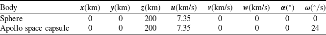
The input parameters for the simulations are presented in Table 2. These input parameters are the same for all the test cases, except for
 $\alpha$
and
$\alpha$
and
 $\omega$
, which are not required for the second test case since it does not consider any tumbling motion. The initial position of the spacecraft is 200km from the Earth’s surface. It is assumed that the spacecraft is initially at a zero angle-of-attack, which is not a binding constraint but rather simply an initial condition that is assumed in the present analysis. The initial angular acceleration is chosen as
$\omega$
, which are not required for the second test case since it does not consider any tumbling motion. The initial position of the spacecraft is 200km from the Earth’s surface. It is assumed that the spacecraft is initially at a zero angle-of-attack, which is not a binding constraint but rather simply an initial condition that is assumed in the present analysis. The initial angular acceleration is chosen as
 $24^{\circ}/\mathrm{s}$
based on observations of orbiting spacecraft [Reference De Pontieu47].
$24^{\circ}/\mathrm{s}$
based on observations of orbiting spacecraft [Reference De Pontieu47].
Table 2. Input parameters for orbital decay simulation

First, a comparison of the orbital decay trajectory of the sphere and Apollo space capsule is discussed to investigate the effect of the geometrical parameters on the trajectory. Next, the effect of assuming a constant
 $C_D$
on the trajectories of both bodies is explored, followed by a comparison of the trajectory of the Apollo space capsule with that of a sphere having the same mass and reference area to analyse the effect of shape on the trajectory. These three case studies are discussed below.
$C_D$
on the trajectories of both bodies is explored, followed by a comparison of the trajectory of the Apollo space capsule with that of a sphere having the same mass and reference area to analyse the effect of shape on the trajectory. These three case studies are discussed below.
Case study I: comparison of trajectories of sphere and Apollo space capsule
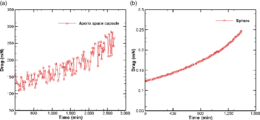
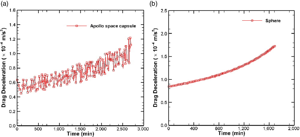
A comparison of the orbital decay trajectories of the two bodies (the sphere and the Apollo space capsule) is shown in Fig. 11 as the variation of altitude with time. Figure 12 shows the drag experienced by the Apollo space capsule and the sphere respectively during their orbital decay. The drag force experienced by the Apollo space capsule is much larger than that experienced by the sphere due to its significantly larger size. On the other hand, the magnitude of the drag deceleration experienced by the Apollo space capsule is comparatively smaller than that experienced by the sphere, as shown in Fig. 13, since the mass of the Apollo space capsule is much larger than that of the sphere. Consequently, the Apollo space capsule has a larger value of the ballistic coefficient (
 $\beta$
) compared with the sphere. Therefore, de-orbiting occurs much faster in the case of the sphere.
$\beta$
) compared with the sphere. Therefore, de-orbiting occurs much faster in the case of the sphere.
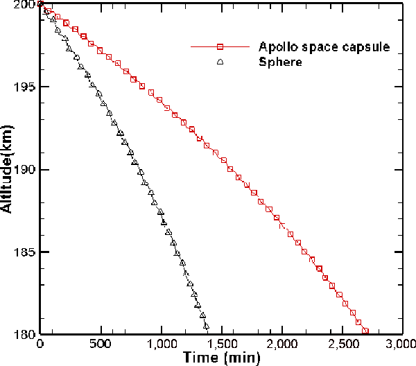
Figure 11. Orbital decay trajectory of Apollo space capsule and sphere.

Figure 12. Drag over time experience by Apollo space capsule and sphere. (a) Apollo space capsule. (b) Sphere.
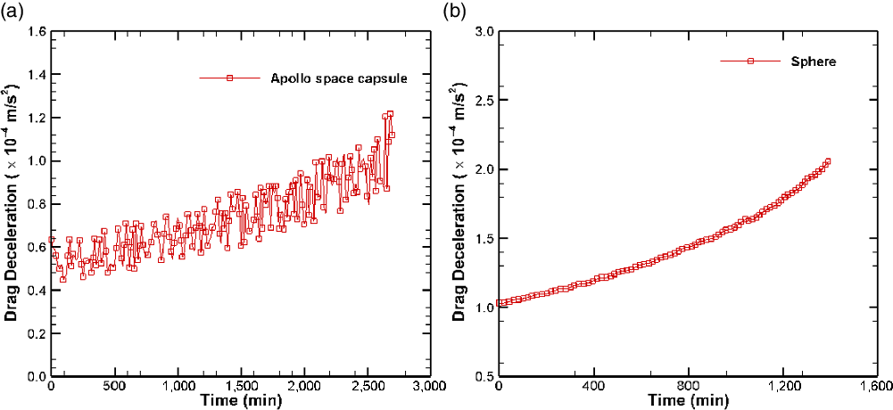
Figure 13. Drag deceleration over time experience by Apollo space capsule and sphere. (a) Apollo space capsule. (b) Sphere.
The fluctuations in the drag and the drag deceleration for the Apollo space capsule, as shown in Figs 12(a) and 13(a), can be explained by the rapid rotation of the body due to the tumbling motion. The variation of the angle-of-attack,
 $\alpha$
, as a result of the tumbling motion is shown in Fig. 14, as the orbit decays with time. The zoomed-in view shown alongside provides further confirmation of the same. The tumbling motion is not applicable for the case of the sphere.
$\alpha$
, as a result of the tumbling motion is shown in Fig. 14, as the orbit decays with time. The zoomed-in view shown alongside provides further confirmation of the same. The tumbling motion is not applicable for the case of the sphere.
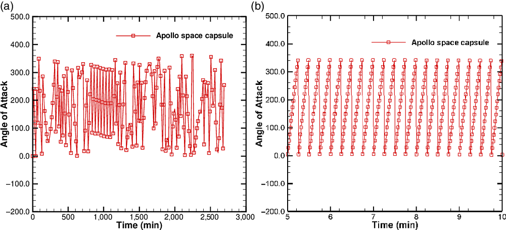
Figure 14. Time variation of the angle-of-attack due to tumbling motion as the orbit decays for Apollo space capsule. A zoomed-in view is shown alongside. (a) Apollo space capsule. (b) Sphere.

Figure 15. Comparison of trajectories for Apollo space capsule and sphere with a constant drag coefficient of 2.2. (a) Apollo space capsule. (b) Sphere.
It is observed from Fig. 12 that the drag force of both bodies increases over time, which leads to an increase in the rate of loss of altitude as the spacecraft descends. This accounts for the increased rate of de-orbiting of both the Apollo space capsule and the sphere as they descend, as is evident from Fig. 11.
The orbital decay of the sphere from a circular orbit at 200km to an altitude of 180km will occur within a day, whereas for a larger spacecraft such as the Apollo space capsule, this will take about twice as long. The chances of surviving re-entry for smaller spacecraft, such as the sphere, are very slim due to aerodynamic heating. As a result, ground impacts of such spacecraft pose a lower risk. Larger spacecraft, such as the Apollo space capsule, have much higher chances of surviving re-entry, thereby posing a risk of ground impact in populated areas. Therefore, controlled re-entry of such spacecraft is necessary to avoid the potential for damage and hazard.
Case study II: effect of drag coefficient on trajectory
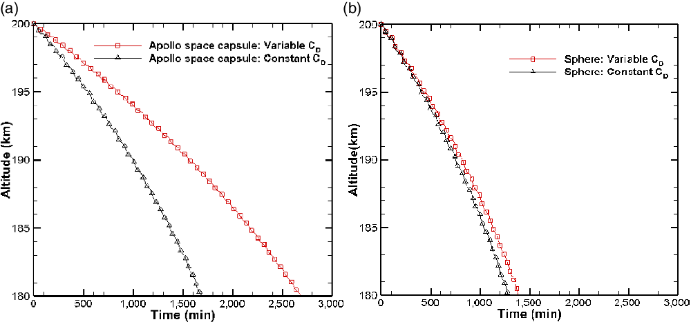
Figure 15 shows the orbital decay trajectory of the sphere and the Apollo space capsule for a constant
 $C_D$
of 2.2 and compares the results with those obtained when
$C_D$
of 2.2 and compares the results with those obtained when
 $C_{D}$
varies. The variation of
$C_{D}$
varies. The variation of
 $C_D$
with the speed ratio is considered for the sphere, whereas the variation of
$C_D$
with the speed ratio is considered for the sphere, whereas the variation of
 $C_D$
with the speed ratio and the angle-of-attack is considered for the Apollo space capsule. It is observed that, for both objects, the calculated orbital decay times for constant
$C_D$
with the speed ratio and the angle-of-attack is considered for the Apollo space capsule. It is observed that, for both objects, the calculated orbital decay times for constant
 $C_D$
deviate from those estimated in the previous section with varying
$C_D$
deviate from those estimated in the previous section with varying
 $C_D$
. Figure 16 shows that, in the case of the sphere, the deviation is comparatively smaller than that for the Apollo space capsule. This can be attributed to the fact that the
$C_D$
. Figure 16 shows that, in the case of the sphere, the deviation is comparatively smaller than that for the Apollo space capsule. This can be attributed to the fact that the
 $C_D$
value obtained for the sphere is close to 2.2, the value assumed for the case of constant
$C_D$
value obtained for the sphere is close to 2.2, the value assumed for the case of constant
 $C_{D}$
. However, when the
$C_{D}$
. However, when the
 $C_D$
values obtained for the Apollo space capsule are analysed, they are found to deviate widely from the 2.2 level. Moreover, the
$C_D$
values obtained for the Apollo space capsule are analysed, they are found to deviate widely from the 2.2 level. Moreover, the
 $C_D$
value of the sphere changes only with the speed ratio but not with the angle-of-attack, while the
$C_D$
value of the sphere changes only with the speed ratio but not with the angle-of-attack, while the
 $C_D$
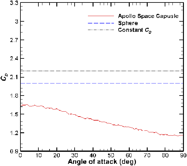
of the Apollo space capsule changes with both the speed ratio and the angle-of-attack. This is clearly evident from Fig. 16. The deviation in the time required for orbital decay indicates the importance of using accurate estimates of
$C_D$
of the Apollo space capsule changes with both the speed ratio and the angle-of-attack. This is clearly evident from Fig. 16. The deviation in the time required for orbital decay indicates the importance of using accurate estimates of
 $C_D$
when calculating decay trajectories.
$C_D$
when calculating decay trajectories.

Figure 16. Variation of
 $C_D$
with angle-of-attack as the body tumbles at a speed ratio of 10. The constant value of
$C_D$
with angle-of-attack as the body tumbles at a speed ratio of 10. The constant value of
 $C_D=2.2$
is shown for reference.
$C_D=2.2$
is shown for reference.
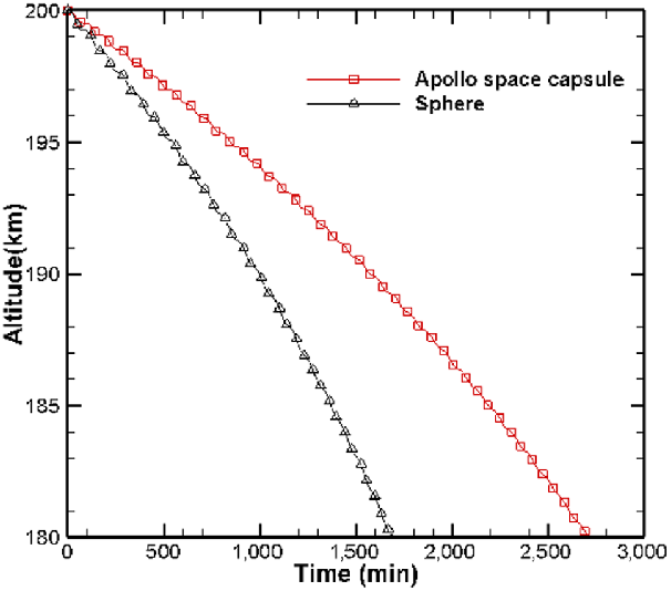
Figure 17. Comparison of trajectories for sphere and Apollo space capsule having same mass and reference area.
Case study III: effect of geometrical shape on trajectory
This case study is undertaken to examine the effect of geometrical shape on the trajectory of tumbling bodies. For this purpose, the reference area and mass of the sphere are kept equal to those of the Apollo space capsule. This allows us to compare the decay trajectories for both bodies having different shapes.
Figure 17 shows the trajectory of the sphere and Apollo space capsule. The current value of
 $C_D$
for both bodies is the same as that in case study I discussed above. It is found that the decay time of the sphere in this case is greatly increased as compared with a regular sphere as discussed in case study I, because of its increased mass and size, which are kept the same as those of the Apollo space capsule. The difference in the orbital decay time between the sphere and Apollo space capsule with the same size and mass is shown in Fig. 17. This occurs because of the difference in the value of
$C_D$
for both bodies is the same as that in case study I discussed above. It is found that the decay time of the sphere in this case is greatly increased as compared with a regular sphere as discussed in case study I, because of its increased mass and size, which are kept the same as those of the Apollo space capsule. The difference in the orbital decay time between the sphere and Apollo space capsule with the same size and mass is shown in Fig. 17. This occurs because of the difference in the value of
 $C_D$
, which is a consequence of the shape of the objects. As seen in case study I, the sphere has a larger
$C_D$
, which is a consequence of the shape of the objects. As seen in case study I, the sphere has a larger
 $C_D$
value as compared with the Apollo space capsule, thus causing a larger drag perturbation to the sphere, as illustrated in Fig. 18. Therefore, the orbital decay rate is faster for the sphere of the same size and mass as the Apollo space capsule.
$C_D$
value as compared with the Apollo space capsule, thus causing a larger drag perturbation to the sphere, as illustrated in Fig. 18. Therefore, the orbital decay rate is faster for the sphere of the same size and mass as the Apollo space capsule.

Figure 18. Drag deceleration over time experienced by Apollo space capsule and sphere having same mass and reference area. (a) Apollo space capsule. (b) Sphere.
5.0 Conclusions
A study is carried out on the orbital decay trajectory of a spacecraft or space debris orbiting in LEO by estimating orbital perturbations due to drag in the rarefied atmosphere using an in-house DSMC solver modified to work in the free molecular regime. Free molecular simulations were performed by using the validated DSMC solver on two common spacecraft with different geometrical specifications, viz. a sphere and an Apollo space capsule, to calculate the aerodynamic coefficients at different speed ratios and angles of attack (for the latter). In the second stage, a general-purpose orbital decay computer program was developed to perform the orbital decay simulation of tumbling bodies. In this work, the tumbling motion of a body is modelled by considering its rotational motion about the pitching axis only. Since the key perturbation considered is drag, which would cause rotation about the pitching axis only, this assumption is reasonable while at the same time improving the numerical efficiency significantly without losing much accuracy. The orbital decay computer program is validated against the period reduction model of Australian IPS Radio and Space Services [Reference Kennewell51].
Orbital decay simulations are performed for three different case studies for both the sphere and Apollo space capsule using a look-up table for the aerodynamics coefficients obtained from the free molecular simulations. In the first case study, orbital decay simulations for a sphere and Apollo space capsule, having widely different shape, size and mass, are performed from a circular orbit of 200km to the onset altitude of re-entry, taken to be 180km. The orbital decay rate is compared between the two bodies. In the second case study, the predicted decay trajectories of the tumbling sphere and Apollo space capsule are compared separately by taking a constant
 $C_D$
value of 2.2. A discrepancy is noted in the orbital decay time for the bodies because, in the free molecular regime,
$C_D$
value of 2.2. A discrepancy is noted in the orbital decay time for the bodies because, in the free molecular regime,
 $C_D$
is a function of the shape and motion of the body. In the third case study, the size and mass of the sphere are changed to the values corresponding to the Apollo space capsule. The orbital decay simulation is performed to analyse the effect of shape on the decay trajectory. It is concluded that the rate of decay of the sphere is slower compared with that observed in the first case. However, the decay time is still faster for the sphere compared with the Apollo space capsule, because of its higher
$C_D$
is a function of the shape and motion of the body. In the third case study, the size and mass of the sphere are changed to the values corresponding to the Apollo space capsule. The orbital decay simulation is performed to analyse the effect of shape on the decay trajectory. It is concluded that the rate of decay of the sphere is slower compared with that observed in the first case. However, the decay time is still faster for the sphere compared with the Apollo space capsule, because of its higher
 $C_D$
value due to its shape.
$C_D$
value due to its shape.
Acknowledgements
The authors acknowledge support from the Science and Engineering Research Board (SERB) through grant no. MTR/2019/000041 and the Indian Space Research Organization (ISRO) through grant STC/AE/2018033. The authors also acknowledge the use of the computing facilities available at the High Performance Computing Facility, Indian Institute of Technology, Kanpur, India.
Conflict of Interest
On behalf of all authors, the corresponding author states that there are no conflicts of interest.